HAL Id: hal-01137820
https://hal.archives-ouvertes.fr/hal-01137820
Submitted on 31 Mar 2015
HAL is a multi-disciplinary open access
archive for the deposit and dissemination of
sci-entific research documents, whether they are
pub-lished or not. The documents may come from
teaching and research institutions in France or
abroad, or from public or private research centers.
L’archive ouverte pluridisciplinaire HAL, est
destinée au dépôt et à la diffusion de documents
scientifiques de niveau recherche, publiés ou non,
émanant des établissements d’enseignement et de
recherche français ou étrangers, des laboratoires
publics ou privés.
Multi-target visual tracking with aerial robots
Pratap Tokekar, Volkan Isler, Antonio Franchi
To cite this version:
Pratap Tokekar, Volkan Isler, Antonio Franchi.
Multi-target visual tracking with aerial robots.
2014 IEEE Int.
Conf, on Intelligent Robots and Systems, Sep 2014, Chicago, United States.
Preprint version, final version at http://ieeexplore.ieee.org/ 2014 IEEE Int. Conf, on Intelligent Robots and Systems, Chicago, IL, USA
Multi-Target Visual Tracking With Aerial Robots
Pratap Tokekar, Volkan Isler and Antonio Franchi
Abstract— We study the problem of tracking mobile targets using a team of aerial robots. Each robot carries a camera to detect targets moving on the ground. The overall goal is to plan for the trajectories of the robots in order to track the most number of targets, and accurately estimate the target locations using the images. The two objectives can conflict since a robot may fly to a higher altitude and potentially cover a larger number of targets at the expense of accuracy.
We start by showing that k ≥ 3 robots may not be able to track all n targets while maintaining a constant factor approximation of the optimal quality of tracking at all times. Next, we study the problem of choosing robot trajectories to maximize either the number of targets tracked or the quality of tracking. We formulate this problem as the weighted version of a combinatorial optimization problem known as the Maximum Group Coverage (MGC) problem. A greedy algorithm yields a 1/2 approximation for the weighted MGC problem. Finally, we evaluate the algorithm and the sensing model through simulations and preliminary experiments.
I. INTRODUCTION
We study the problem of tracking multiple moving targets using aerial robots. We consider the scenario where cameras that face downwards are mounted on the robots to track targets moving on the ground plane. A robot can potentially track more targets by flying to a higher altitude, thus in-creasing its camera footprint. However, this may reduce the quality of the view due to the increased distance between the cameras and the targets. There is a trade-off between the number of targets tracked and the corresponding quality of tracking. We investigate this trade-off and present an approximation algorithm for multi-target tracking.
We start by showing that it may not always be possible to track all targets while always maintaining the optimal quality of tracking (or any factor of the optimal quality), even if the targets’ motion is fully known. Hence, we focus on the following two variants: maximize the number of targets tracked subject to a desired tracking quality per target, and maximize the sum of quality of tracking for all targets. The two problems can be formulated as the unweighted and weighted versions of the Maximum Group Coverage Problem (MGC). A simple greedy approach provides a 1/2 approximation to unweighted MGC [1]. We show that the approximation guarantee also holds for the weighted case which allows a practical solution to the trajectory planning
P. Tokekar and V. Isler are with the Department of Computer Science &
Engineering, University of Minnesota, U.S.A.{tokekar,isler} at
cs.umn.edu
A. Franchi is with the Centre National de la Recherche Scientifique (CNRS), Laboratoire d’Analyse et d’Architecture des Syst`emes (LAAS),
France.antonio.franchi at laas.fr
This material is based upon work supported by the National Science Foundation under Grant Nos. 1317788 and 1111638.
problem with provable performance guarantees. We evaluate the algorithm in simulations and preliminary experiments with an indoor platform using four aerial robots.
The rest of the paper is organized as follows. We begin with the related work in Section II. The problem setup and a discussion of the sensing quality are presented in Section III. The infeasibility of tracking all targets with a constant factor of the optimal quality is proven in Section IV. The tracking algorithm is presented in Section V, and evaluated through simulations and preliminary experiments in Sections VI and VII respectively. Section VIII concludes the paper.
II. RELATEDWORK
Target tracking is an important problem for robotics, and has been widely studied under different settings. Spletzer and Taylor [2] considered the problem of tracking multiple mobile targets with multiple robots. They presented a general solution based on particle filtering in order to choose robot locations for the next time step that maximizes the quality of tracking. Frew [3] studied the problem of designing a robot trajectory, and not just the next robot location, in order to maximize the quality of tracking a single moving target. LaValle et al. [4] studied the problem of maintaining the visibility of a single target from a robot for the maximum time. Gans et al. [5] presented a controller that can keep up to three targets in one robot’s field-of-view.
When the motion of the targets is fully known, the tracking problem can be formulated as a kinetic facility location problem. The goal of the stationary version is to place k facilities (robots) given the location of n sites (targets), so as to minimize the maximum distance between a facility and a site. For the kinetic version, Bespamyatnikh et al. [6] and Durocher [7] presented approximation algorithms to control respectively one and two mobile facilities, when the trajectories for the sites are given. Recently, de Berg et al. [8] presented improved approximation algorithms with two mobile facilities when only an upper bound on the velocities of the sites is available. However, the general problem of kinetic facility location withk facilities is open. In the extreme case where no prior information of the targets is available, the multi-robot tracking problem can be formulated as a coverage problem [9]. Schwager et al. [10] presented strategies to control the position and orientation of overhead cameras mounted on aerial robots in order to achieve equal visual coverage of the ground plane.
Unlike previous works, we study the trade-off between quality of tracking, and the number of targets tracked. We present an algorithm that chooses trajectories for each robot, instead of choosing just the next best location. This algorithm
-1 0 1 -1 0 1 0 1 2 3 4 5 6 X(m) R1 Y(m) Z(m) (a) -10 0 1 2 3 0.5 1 1.5 2 2.5 3 3.5 4 Area =0.11 Area =0.23 Area =0.26
Uncertainty due to noise in yaw +/- π/24
(b) -5 -4 -3 -2 -1 0 1 2 3 4 5 -5 -4 -3 -2 -1 0 1 2 3 4 5
maximum noise in position +/- [0.2,0.2,0.2] maximum noise in orientation +/- [π/24,π/24,π/24]
X(m) Y(m) 4 6 8 10 12 14 16 18 20 (c)
Fig. 1. (a) Backprojection from a pixel yields a pyramid. (b) Uncertainty in target’s estimate due to uncertain yaw angle of the robot. (c) Map showing
the area of projection for the true target at[x, y, 0] (best viewed in color).
The camera pose is estimated to have position[0, 0, 5] m and roll, pitch and
yaw angles as0 radians. Maximum image noise is ±5 pixels.
can be applied to the following two versions of the problem: tracking maximum number of targets, and maximizing the quality of tracking. We begin by formulating the problem and describing the sensing model.
III. PRELIMINARIES ANDPROBLEMFORMULATION
Letk denote the number of robots, and n denote the total number of targets in the environment. The position of any robot or target is specified by their 3D coordinates x, y, z. The position of theith robot at timeτ is denoted by r
i(τ ).
Letzmin be the minimum flying altitude. All robots have a
camera that faces downwards. Let φ represent the field-of-view angle for the cameras. We assume that the robots can communicate amongst each other at all times.
Let ti(τ ) denote the position of the ith target. ti(τ ) is
given by the position of a reference point that the robots can use to uniquely identify any target. For example, the reference point can be the centroid of a colored patch or a unique feature point on the object. All targets always move on the ground plane, i.e.,z = 0 for all ti.
The reference point of any targetti in the field-of-view of
a robot projects to some pixel in the image. A pixel can be backprojected to a ray in the world frame. In general, with no other information, it is not possible to solve for the target’s location along this ray with a single camera measurement. However, since we assume that all targets move on the ground plane, we can solve for the coordinates ofti.
Ideally, we can exactly estimate ti given an image
mea-surement, the camera pose, and the projection matrix. In practice, however, the following factors lead to an uncertain estimate ofti:
(1) The backprojection of camera pixels, which have quan-tized, integer coordinates, is not longer single ray but a pyramid (Figure 1(a)).
(2) Pixel measurements may be corrupted by noise. If the maximum noise is bounded by ∆p pixels, we backproject the set of pixels±∆p around the measured pixel. The true target location is contained within the larger backprojection. (3) The pose of the camera (or the robot) may not be accurately known. Typically, using exteroceptive sensors such as GPS and compass, we can bound the maximum uncertainty in estimating the robot pose. When the robot pose
is known up to a bounded uncertain set, we can compute the backprojection for each pose within the set (Figure 1(b)).
In general, the quality of tracking under the three sources of errors, is a function of the relative distance and angle between the robot and the target, as seen in Figure 1(c). For a given true location of the target and an estimate of the robot pose, Figure 1(c) plots the maximum area of backprojection over all possible noisy measurements of the target, and all possible true robot poses.
While tracking, robots only have an estimate of the true target position. The uncertain estimate can be represented as a set of possible target locations on the ground plane. Given a motion model, the robots can propagate the set to obtain predicted target position, e.g., using particle filtering [11]. The maximum area of backprojection can be computed for each predicted target position as shown in Figure 1(c).
The quality of tracking for a given target and robot pair can be defined as some measure of the areas of backprojection found for a predicted target position. Let qi(rj, τ ) denote
the measure for targettiand robotrj at timeτ . The quality
of trackingti at τ , is given by the best quality of tracking
amongst all robots tracking ti, i.e.,qi(τ ) = maxjqi(rj, τ ).
Finally, the total quality of tracking atτ is given by the sum of quality over all targetsQ(τ ) =P∀iqi(τ ) over all targets.
Alternatively, we may also consider the bottleneck quality over all targetsQ(τ ) = miniqi(τ ).
IV. INFEASIBILITY OFTRACKINGALLTARGETS
In this section, we show the infeasibility of tracking all targets while maintaining any constant factor approximation of the optimal quality of tracking. We prove this by construct-ing an instance where the two goals, track all targets and maximize quality of tracking, conflict each other. We create a simple instance on a line where the quality of tracking is inversely proportional to the distance between the robot and the target: qi(rj, τ ) = 1/d(ti(τ ), rj(τ )) if ti is in the
field-of-view ofrj, andqi(rj, τ ) = 0 otherwise. The overall
quality of tracking will be given by the bottleneck quality Q(τ ) = miniqi(τ ).
We use the instantaneous optimal quality of tracking, Q∗(τ ), as the baseline for comparison. Q∗(τ ) is the quality
of tracking at τ , if one were to optimally place all the cameras at any location for anyτ , regardless of their loca-tions beforeτ . The placement of k cameras achieving Q∗(τ )
may be significantly different from the placement achieving Q∗(τ − ǫ). There may or may not exist k continuous
robot trajectories achieving Q∗(τ ). Nevertheless, Q∗(τ ) is
an upper bound on the quality of tracking. This raises the question of whether we can at least maintain a constant-factor approximation ofQ∗(τ ) while tracking all targets. The
theorem given next shows this is not possible, even when the motion of the targets is fully known.
Theorem 1 LetQ∗(τ ) be the instantaneous optimal quality
of tracking at time τ . Let the maximum speed of all targets
bev. For any 0 < α≤ 1 and β > 0, no algorithm can track
alln > k targets with at least αQ∗(τ ) quality for all τ with
k≥ 3 robots having a maximum speed of βv.
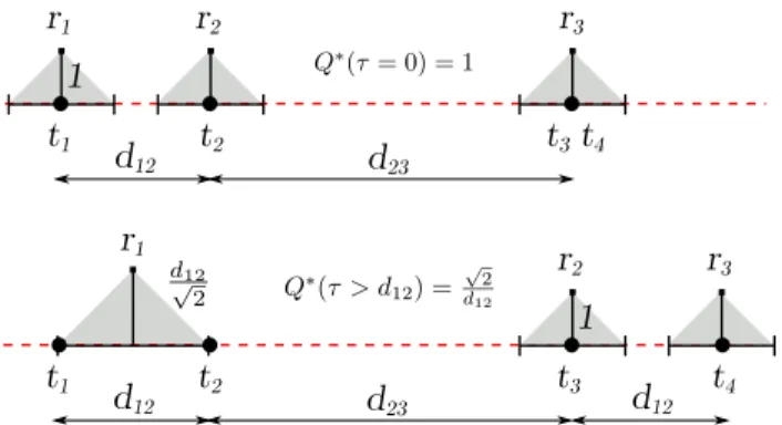
Proof: Consider Figure 2. We have k = 3 robots and n = 4 targets on a line. The distance between t3 and t4
is 0 at time0. Targets t1, t2 andt3 remain stationary at all
times, and t4 moves with v = 1 to the right on the line.
zmin= 1 and φ = π/4 denote the minimum flying altitude
and field-of-view angles (Section III).
Fig. 2. At τ= 0, t3 and t4 are covered by the same robot to achieve
Q∗(0), where as for τ > d
12, t3 and t4are covered by separate robots.
If we have 4 targets and 3 robots, then there must exist a robot covering at least two targets at any given time. At τ = 0, we can verify that the optimal algorithm uses separate robots to cover t1 and t2, and one robot to cover t3 and
t4 (Figure 2). That is, Q∗(0) = 1. Similarly, for any time
τ > d12, optimal uses separate robots to cover t3 and t4,
and same the robot to covert1 andt2 makingQ∗(τ ) = √2 d12.
Thus, in any optimal algorithm, of the two robots cov-ering t1 and t2, one will switch to cover either t3 or t4,
after τ = d12. An approximation algorithm, on the other
hand, does not necessarily have to make the same switch.
Nevertheless, by settingd12appropriately, we will show that
any approximation algorithm will be required to make the same switch at some time. By makingd23sufficiently large,
we will show that such a switch is infeasible with bounded velocity robots. The rest of the proof shows the existence of appropriated12andd23values. This construction is similar to
the one used by Durocher [7] to prove the inapproximability of the kinetick–center problem. For the case of aerial robots, however we show how to additionally take into account non-zerozmin andφ values.
Let ALG be any algorithm that maintains a qualityQ(τ )≥ αQ∗(τ ). If we set d12>√2
α , then ALG cannot use the same
robot to covert1 and t2 at time τ = 0. Else, Q(0) < α =
αQ∗(0) which violates the approximation guarantee. Hence,
ALG uses separate robots to covert1 andt2 at time0.
Similarly, we can show that for any timeτ > d12 α , ALG
must use separate robots to cover t3 and t4. Else Q(τ ) < √2
τ < αQ∗(τ ) violating the approximation guarantee.
One of the two separate robots, say r, covering t1 and
t2 initially, must cover eithert3 andt4 at time τ > dα12. In
timeτ , r must travel at least d23− 1 α− d12 √ 2α distance. Here, 1 α and d12 √
2α come from the condition that Q(0) ≥ α and
Q(τ )≥ α√2 d12.
Consider a timeτ = 2d12
α . At this time,r covers a
maxi-mum distance ofβτ = β2d12 α . Setd23> β 2d12 α + 1 α+ d12 √ 2α.r
cannot simultaneously cover at least one oft1ort2at time0,
and at least one oft3ort4at timeτ , which is a contradiction.
Hence, ALG cannot maintain anα approximation of Q∗ for
all times.
The instance created in the proof above uses minimum flying altitude zmin = 1 and camera field-of-view angle
φ = π/4. We can create corresponding instances for any other values of these parameters. In light of Theorem 1, we drop the requirement that all targets must always be tracked. Instead we focus on the case when the robots are allowed to track a fraction of all targets.
V. 1/2 APPROXIMATIONALGORITHM
In this section, we present the main algorithm to maximize the number of targets tracked, or maximize the quality of tracking. We divide the time into rounds of fixed duration. We consider the scenario where using measurements from previous rounds, the robots are able to predict the motion of the targets for the current round. For each robot, we create a set ofm candidate trajectories that can be followed for the current round. For example, these trajectories can be generated using existing grid-based or sampling-based methods [12]. Our goal is to choose a trajectory for each of the robots for the current round.
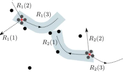
Figure 3 shows a simple instance with two robots, and three candidate trajectories each robot can follow. The cam-era footprint along two such trajectories as well as the set of targets covered by these trajectories are shown. Note that the trajectories need neither be restricted to any discretized grid, nor have uniform length or uniform speed.
LetRj(x) denote the set of targets predicted to be covered
by xth trajectory followed by jth robot. We create a set
system (X,R) where X is the set of all targets and R is a collection of all Rj(x) sets. We group sets in R into k
collections, one per robot. Each group containsm sets each. That is,
R = { R1(1), . . . , R1(m)
| {z }
candidate trajectories for r1
, . . . , Rk(1), . . . , Rk(m)
| {z }
candidate trajectories for rk
} (1) A valid assignment of trajectories can be represented by a map,σ : [1, . . . , k]→ [1, . . . , m], indicating trajectory σ(j) (i.e., the setRj(σ(j))) is chosen for the jth robot. We can
remove a target from the set Rj(x) if it does not satisfy a
given minimum quality of tracking requirement.
A. Maximizing Number of Targets
First consider the case of maximizing the number of targets tracked byk robots. This problem is a generalization of the maximum coverage problem [13] stated as: choosek
subsets to maximize the cardinality of the union of all subsets. In our case, we cannot arbitrarily pickk subsets since they must belong to distinct groups (i.e., the same robot cannot be assigned to two trajectories).
The maximum coverage problem, under group constraints, can be stated as: choose k subsets of R given by a map,
Fig. 3. At the start of each round, we have a set of m candidate trajectories per robot. The trajectories may be non-uniform and of varying speeds. Using the predicted motion of the targets, we can determine which targets will be covered for a given trajectory and the corresponding quality of tracking.
σ : [1, . . . , k]→ [1, . . . , m] such that the union of all subsets
is maximized. The constraint that the same robot cannot
be assigned to two trajectories is enforced by requiring the output be a mapσ. This problem is known as the Maximum Group Coverage (MGC) problem. Chekuri and Kumar [1] proved that the greedy algorithm yields a1/2 approximation for MGC. Their algorithm can directly be applied to track half the number of targets as an optimal algorithm. Our contribution is to extend the analysis to the weighted case.
B. Maximizing Quality of Tracking
For the case of maximizing the overall quality of tracking, we formulate a weighted version of MGC. Letqi(Rj(x)) be
the quality of tracking targetti with robotrj following the
xth
trajectory.qi(Rj(x)) can represent the expected quality
of tracking as described in Section III. The weight of any setRj(x)∈ R is given by the sum of qualities of all targets
tracked byRj(x). The objective is to maximize the sum of
quality of tracking for all targets1.
The greedy algorithm for the unweighted MGC can be modified for the weighted setting (Algorithm 1). In each iteration, we choose a set Rj(x) greedily that maximizes
the total weight. We add Rj(x) to the solution, and discard
all other sets belonging to the same group, i.e., all other candidate trajectories for the same robotrj. This proceeds
until we have chosen a trajectory for all robots. Algorithm 1: Greedy Weighted MGC Algorithm
1 C← ∅, I ← ∅ 2 forp = 1 to k do
3 Find Ri(x) such that Q(Ri(x)∪ C) is greatest, and
i6∈ I 4 σ(i)← x 5 C← C ∪ Ri(x) 6 I← I ∪ {i} 7 end 8 Returnσ
Theorem 2 Algorithm 1 gives a (1/2− ǫ) approximation
for the weighted MGC problem for anyǫ > 0 in polynomial
time.
1The bottleneck version of maximizing the minimum quality of tracking
over all targets cannot be applied since not all targets are tracked.
The analysis by Chekuri and Kumar [1] for the unweighted case can be modified for this weighted case. We present our full proof in the accompanying technical report [14], for completeness.
We now evaluate the greedy algorithm through simulations and preliminary experiments.
VI. SIMULATIONS
In this section, we describe our implementation of the algorithm, and evaluate its performance through simulations. We carried out the simulations using the SwarmSimX sim-ulation environment [15]. SwarmSimX is a real-time multi-robot simulator designed for modeling rigid-body dynamics in 3D environments. Models of the MikroKopter Quadrotor2 were used to simulate the motion of the robots.
For simulating the targets, we generated random trajecto-ries as follows. Each target randomly chooses a speed and direction and moves along this direction for a random interval of time, drawn from a normal distribution. This class of trajectories is motivated by wildlife monitoring applications, where foraging animals have been found to follow such mobility models [16]. The mean and standard deviation of the normal distribution were set to10 s and 1 s, respectively in the simulations.
The target trajectories were restricted to20× 20 m square on the ground plane. The initial locations of all targets were chosen uniformly at random near the robot locations. A moving average filter of window length 5 running at 10 Hz was used to estimate the position and velocity of the observed targets for the next planning round. A measurement for a target was obtained only if it was contained within the field-of-view of some robot.
For each robot, we created the following set of candidate trajectories: (a) stay in place, and (b) radially symmetric along8 horizontal directions with a speed of 0.5 m/s. Thus, each robot could choose from a set of 9 trajectories in a round. Each round was set to a duration of 2 s. A trial consisted of50 rounds.
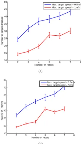
Figures 4(a) and 4(b) show the effect of the number of robots and the maximum speed of the targets. As expected, the number of tracks and quality of tracking increases as the number of robots increase. Increase in the maximum speeds of the targets has the effect of spreading them further apart, which further reduces the number of targets that can be tracked. For these trials, the height of the robots was fixed to 3.5 m (i.e., the size of the camera footprint was fixed). Figure 5 shows the total number of targets tracked in one representative trial as a function of the time. Once the robots have lost track of a particular target, they do no receive any position information about that target. Thus, they cannot predict the future locations for a lost target, unless it appears again in the field-of-view of some robot.
For the simulations, we did not incorporate the uncer-tainty due to sensing. In the next section, we validate the uncertainty model and present results from a preliminary experiment using4 aerial robots.
2http://mikrokopter.de
1 2 3 4 5 6 7 8 10 15 20 25 30 35 40 45 50 Number of robots
Number of targets tracked
Max. target speed = 0.5m/s Max. target speed = 1m/s
(a)
(b)
Fig. 4. (a) Number of targets covered out of50 targets in the environment.
(b) The average quality of tracking. The weight qi(Rj(x) is computed as
the inverse of the minimum distance between the target and the robot along
Rj(x).
VII. EXPERIMENTS
In order to validate our sensing model and the algorithm, we performed trials on an indoor setup (Figure 6). The setup consisted of four quadrotors controlled using the TeleKyb framework [17]. All robots communicated directly with a central computer via a wireless XBee link. Each robot was fitted with a downward facing camera. The cameras streamed the live images wirelessly directly to the central computer. An indoor motion capture system was used for position feedback, while orientation is stabilized onboard.
A. Validating the Sensing Model
We first conducted trials to validate the sensing model presented in Section III. A robot was programmed to fly along a given trajectory at heights of 1 m and 1.5 m. The motion of the robot was smoothed, so as to ensure that the roll and pitch angles remained close to zero. Colored balls were placed on the ground (Figure 6). The pink and the yellow colored balls were fixed to motion capture markers to record their ground truth locations. All cameras were calibrated to obtain they camera parameters.
Figure 7 shows an image obtained using the on-board camera, along with the estimated and true locations of the balls. The backprojection area was computed considering±5
0 20 40 60 80 100 0 5 10 15 20 25 30 Time in sec
Number of targets covered
Fig. 5. The number of targets tracked in one trial. As the targets spread the total number of targets that can be tracked decreases. Once a target moves out of the field-of-view, the robots cannot predict their future locations.
Fig. 6. Experimental setup. Each robot is fitted with a downward facing
wireless camera. All robots directly communicate with a central computer.
maximum measurement error in pixels, ±5 cm maximum error in robot position, ±π/18 radians maximum error in the yaw angle, and ±π/48 radians maximum error in the roll and pitch angles. The average area of backprojection (for 50 images which contained either the yellow or pink balls) was0.46 m2
. The average error between the centroid of the projected area and the true location was0.28 m, with a standard deviation of0.3 m.
B. Tracking Experiment
We implemented the greedy algorithm on the four robots. The controller on-board the robot was set to operate the robots smoothly in near-hovering mode at an average speed 0.5 m/s. Each round lasted for 3 seconds. The pink and yellow balls were moved manually (Figure 6). For this trial,
(a) -3 -2 -1 0 1 2 3 -3 -2 -1 0 1 2 3 Area =0.76 Area =1.2 X(m) Y(m) (b)
Fig. 7. Validating the sensing model. (a) On-board camera image. (b) The
true target location (colored circles) in the global frame, and the estimated locations using the method described in Section III.
-2 -1.5 -1 -0.5 0 0.5 1 1.5 2 -3 -2 -1 0 1 2 3 R1 R2 R3 R4 X(m) Y(m) t=110 secs -2 -1.5 -1 -0.5 0 0.5 1 1.5 2 -3 -2 -1 0 1 2 3 R1 R2 R3 R4 X(m) Y(m) t=113 secs
(a) At t= 110 s, R3 chose the trajectory moving to the left to
keep tracking the yellow target.
-2 -1.5 -1 -0.5 0 0.5 1 1.5 2 -3 -2 -1 0 1 2 3 R1 R2 R3 R4 X(m) Y(m) t=119 secs -2 -1.5 -1 -0.5 0 0.5 1 1.5 2 -3 -2 -1 0 1 2 3 R1 R2 R3 R4 X(m) Y(m) t=123 secs
(b) At t= 119 s, R1chose the trajectory moving to the right to
keep tracking the pink target.
Fig. 8. Start (left figures) and end (right figures) of two rounds. Dashed
trail shows the locations of the robots and targets in the preceding 5 secs.
the locations of the targets were obtained from the motion capture system. The robots used a moving average filter to predict the locations of the targets, based on previous measurements. A radius of √2 m was found empirically to correspond to the camera footprint when the robots operated at a height of 2.5 m. The robots had one of the four grid neighbors in the z = 2.5 m plane as candidate trajectories.
Figure 8 shows the locations of the robots and the targets before and after two key rounds: at times 110 s and 119 s. The two rounds show events when the robots predicted that the target would move out of the coverage area in the next round. Hence, as an outcome of the greedy algorithm, the robots chose corresponding trajectories in order to continue to track the targets.
The sensing validation and tracking trials presented here demonstrate a proof-of-concept implementation of the com-ponents of our system. Our ongoing efforts are directed to-wards performing large scale experiments with this system.
VIII. CONCLUSION
In this paper, we studied a visual tracking problem in which a team of robots equipped with cameras are charged with tracking the locations of targets moving on the ground. We discussed the sources of uncertainty that affect the quality of estimating the locations of ground targets using overhead images. We showed the infeasibility of tracking all targets while maintaining the optimal quality of tracking, or any factor of the optimal quality, at all times. We then formulated the target tracking problem where the goal is to assign trajectories for each robot in order to maximize the quality of tracking. When we are given a set of candidate robot trajectories, we showed how the problem can be posed as a combinatorial optimization problem. A simple and easy-to-implement greedy algorithm applied to this problem yields a 1/2 approximation. Finally, we presented results from sim-ulations and preliminary experiments validating the sensing
model and demonstrating the feasibility of implementing the algorithm. Future work includes investigating the problem under inter-robot communication constraints, and conducting larger scale experimental validation.
IX. ACKNOWLEDGEMENTS
We thank the Max Planck Institute for Biological Cyber-netics in Germany, for the experimental setup, and Simon Hartmann and Massimo Basile for their help during the experiments.
REFERENCES
[1] C. Chekuri and A. Kumar, “Maximum coverage problem with group budget constraints and applications,” in Approximation, Randomiza-tion, and Combinatorial Optimization. Algorithms and Techniques. Springer, 2004, pp. 72–83.
[2] J. R. Spletzer and C. J. Taylor, “Dynamic sensor planning and control for optimally tracking targets,” The International Journal of Robotics Research, vol. 22, no. 1, pp. 7–20, 2003.
[3] E. W. Frew, “Observer trajectory generation for target-motion estima-tion using monocular vision,” Ph.D. dissertaestima-tion, Stanford University, 2003.
[4] S. M. LaValle, H. H. Gonz´alez-Banos, C. Becker, and J.-C. Latombe, “Motion strategies for maintaining visibility of a moving target,” in IEEE International Conference on Robotics and Automation, vol. 1. IEEE, 1997, pp. 731–736.
[5] N. R. Gans, G. Hu, K. Nagarajan, and W. E. Dixon, “Keeping multiple moving targets in the field of view of a mobile camera,” IEEE Transactions on Robotics, vol. 27, no. 4, pp. 822–828, 2011. [6] S. Bespamyatnikh, B. Bhattacharya, D. Kirkpatrick, and M. Segal,
“Mobile facility location,” in Proceedings of the 4th International Workshop on Discrete Algorithms and Methods for Mobile computing
and Communications. ACM, 2000, pp. 46–53.
[7] S. Durocher, “Geometric facility location under continuous motion,” Ph.D. dissertation, The University of British Columbia, 2006. [8] M. de Berg, M. Roeloffzen, and B. Speckmann, “Kinetic 2-centers
in the black-box model,” in Proceedings of the 29th Annual on
Symposium on Computational Geometry. ACM, 2013, pp. 145–154.
[9] S. Martinez, J. Cortes, and F. Bullo, “Motion coordination with distributed information,” IEEE Control Systems, vol. 27, no. 4, pp. 75–88, 2007.
[10] M. Schwager, B. J. Julian, M. Angermann, and D. Rus, “Eyes in the sky: Decentralized control for the deployment of robotic camera networks,” Proceedings of the IEEE, vol. 99, no. 9, pp. 1541–1561, 2011.
[11] S. Thrun, W. Burgard, D. Fox, et al., Probabilistic robotics. MIT
press Cambridge, 2005, vol. 1.
[12] C. J. Green and A. Kelly, “Toward optimal sampling in the space of paths,” Springer Tracts in Advanced Robotics, vol. 66, pp. 281–292, 2010.
[13] D. S. Hochbaum and A. Pathria, “Analysis of the greedy approach in problems of maximum k-coverage,” Naval Research Logistics, vol. 45, no. 6, pp. 615–627, 1998.
[14] P. Tokekar, V. Isler, and A. Franchi, “Multi-target visual tracking with aerial robots,” Department of Computer Science & Engineering,
University of Minnesota, Tech. Rep. 14-013, June 2014,http://www.
cs.umn.edu/research/technical reports/view/14-013.
[15] J. L¨achele, A. Franchi, H. H. B¨ulthoff, and P. Robuffo Giordano, “SwarmSimX: Real-time simulation environment for multi-robot sys-tems,” in 3rd International Conference on Simulation, Modeling, and Programming for Autonomous Robots, Tsukuba, Japan, Nov. 2012. [16] S. Benhamou, “How many animals really do the levy walk?” Ecology,
vol. 88, no. 8, pp. 1962–1969, 2007.
[17] V. Grabe, M. Riedel, H. H. B¨ulthoff, P. Robuffo Giordano, and A. Franchi, “The TeleKyb framework for a modular and extendible ROS-based quadrotor control,” in 6th European Conference on Mobile Robots, Barcelona, Spain, Sep. 2013, pp. 19–25.