Classification of Sound Textures
Nicolas Saint-ArnaudBachelor of Electrical Engineering Universit6 Laval, Qu6bec, 1991
Master of Science in Telecommunications
INRS-Telecommunications, 1995
Submitted to the Program in Media Arts and Sciences, School of Architecture and Planning, in partial fulfillment of the requirements for the degree of
Master of Science at the Massachusetts Institute of Technology September 1995 ©Massachusetts Institute of Technology, 1995
r''
-Author Nicolas Saint-Arnaud
Program in Media Arts and Sciences August 23, 1995
Certified by
/
Barry L. VercoeProfessor, Program in Media Arts & Sciences Thesis Supervisor
Stephen A. Benton Chair, Departmental Committee on Graduate Students Program in Media Arts and Sciences 'L*AAHUSETTS INS4riUTE
OF TECHNOLOGY
OCT 2
6
1995
a&tk
LIBRARIES
Classification of Sound Textures
byNicolas Saint-Arnaud
Submitted to the Program in Media Arts and Sciences,
School of Architecture and Planning
on August 23, 1995
in partial fulfillment of the requirements for the degree of
Master of Science
Abstract
There is a class of sounds that is often overlooked, like the sound of a crowd or the rain. We refer to such sounds with constant long term characteristics as Sound Textures (ST). This thesis describes aspects of the human perception and machine processing of sound textures.
Most people are not adept at putting words on auditory impres-sions, but they can compare and identify sound textures. We per-formed three perception experiments on ST's. A Similarity Experiment let us build a map where symbols that are close corre-spond to ST that are perceived similar. A Grouping Experiment pro-vided groups of ST's that share a characteristic and a name; we call these groups P-classes. Finally, an Trajectory Map(Richards) Experi-ment points to some features used by subjects to compare ST's.
For machine processing, we look at two levels: local features, which we call Sound Atoms, and the distribution of Sound Atoms in time. In the implemented classification system, the low-level analysis is done by a 21-band constant-Q transform. The Sound Atoms are magnitude of points in the resulting time-frequency domain. The high level first builds vectors which encode observed transitions of atoms. The transition vectors are then summarized using a Cluster-based Probability Model (Popat and Picard). Classification is done by comparing the clusters of models built from different sound textures. On a set of 15 ST's, the classifier was able to match the samples from different parts of the same recording 14 times. A preliminary system to make a machine name the P-class of an unknown texture shows promise.
Thesis Advisor: Barry Vercoe
Title: Professor, Program in Media Arts and Sciences
Classification of Sound Textures
by
Nicolas Saint-Arnaud
Thesis Reader Rosalind W. Picard
Associate Professor Program in Media Arts & Sciences
Thesis Reader Whitman A. Richards
Head Program in Media Arts & Sciences
Acknowledgments
So many people had a tangible effect on this work that it seems im-possible to thank them all and enough. Thanks to:
e my parents for their patience and support, * the Aardvarks who put the fun in the work, * all my friends, for the smiles and support,
e prof. W.F. Schreiber for continued support and interesting conversations, and Andy Lippman for a decisive interview, * Linda Peterson, Santina Tonelli and Karen Hein without
whom we would probably fall of the edge of the world, e the Machine Listening Group, a fun bunch,
e my advisor, Barry Vercoe,
* my readers for their enthusiasm and helpful hints,
e Kris Popat and Roz Picard for the numerous and inspiring discussions and ideas for research topics, and for their help with the cluster-based probability model,
e Stephen Gilbert and Whitman Richards for their help with the Trajectory Mapping experiments,
e Dan Ellis, for tools, figures and sound advice, e all who volunteered as human subjects,
Table of Contents
A bstra ct ... 2
A cknow ledgm ents ... 4
T a bl e of C o nte nts ... 5 L ist of F ig u re s ... 9 L ist of T a ble s ... 1 1
Chapter 1 Introduction...
12
1.1 Motivation ... 12 1.2 Overview... 13 1.3 Background... 14Connection to Other Groups at the Media Lab 1.4 Applications ... 15
1.5 Summary of Results ... 16
Human Perception Machine Classification
Chapter 2 Human Perception of Sound Textures...17
Chapter Overview 2.1 What do You Think is a Sound Texture?... ... . . 17
Dictionary Definition 2.1.1 Examples ... 18
Texture or Not? 2.1.2 Perceived Characteristics and Parameters... 19
Properties Parallel with Visual Texture Parameters 2.1.3 Classes and Categories ... 22
2.2 Working Definition of Sound Textures ... 23
Too Many Definitions 2.2.1 Working Definition of Sound Texture ... 23
First Time Constraint: Constant Long-term Characteristics Two-level Representation Second Time Constraint: Attention Span Summary of our Working Definition 2.3 Experiments with Human Subjects ... 26
Goal 2.3.1 Common Protocol ... 26
Shortcomings 2.4 Similarity Experiment ... 26
2.4.1 Method: Multidimensional Scaling (MDS) ... 27 Protocol
2.4.2 Results ... 29 Proof of Principle of the MDS Algorithm
2.5 Grouping Experiment... 34 Goal
2.5.1 Protocol ... 34 First Grouping Experiment
Second Grouping Experiment
2.5.2 Results ... 35 2.6 Ordering Experiment... 38
Goal
2.6.1 Method: Trajectory Mapping (TM)... 38 Protocol
2.6.2 Results ... 41 2.7 P-classes ... 43
Chapter 3 Machine Classification of
Sound Textures
...
46
Chapter Overview
3.1 A Two-Level Texture Model ... 46 Key Assumption
3.2 Low Level: Sound Atoms... 47 3.2.1 Kinds of Atoms ... 48
Signal-Specific Atoms Generalized Atoms Filterbanks
Energy Groupings in Time and Frequency
3.3 A 21-band Constant-Q Filterbank... 50 Hilbert Transform
3.4 High Level: Distribution of Sound Atoms ... 53 Periodic and Random
Cluster-Based Probability Model Modeling feature transitions (Analysis)
3.5 Cluster-Based Probability Model ... 55 3.5.1 Overview ... 55
Cluster-Based Analysis Example in 1 Dimension Approximation by clusters
3.5.2 Description ... 58 Two-dimensional Feature space
Conditional Probabilities Approximation by clusters
3.5.3 Classification ... 62
Model Comparison Distance Measures Dissimilarity Measure Closest Known Texture Classification into P-classes Classifier training: Classification: 3.5.4 Evaluating Classification success ... 63
Chapter 4 Machine Classification Results
...
64
Chapter Overview 4.1 P rotocol ... 64 4.1.1 Set of Signals ... 64 Training Set Testing Set 4.1.2 Extracting Atoms ... 65
4.1.3 Spectrograms of the Sound Texture Samples ... 66
4.1.4 Modeling Transitions ... 70
4.1.5 Comparing Cluster-based Models... 71
4.2 Results... 72
4.2.1 Dissimilarities within the Training Set... 72
MDS 4.2.2 Classification to Closest in Training Set... 73
4.2.3 Classification into P-classes... 75
4.3 Discussion ... 76
Chapter 5 Future Directions
...
78
Chapter Overview 5.1 Better Atoms ... 78
Energy Groupings in Time and Frequency Harmonics, Narrow-band Noise, Impulses 5.2 Ideas for Classification... 80
5.2.1 Multiresolution Modeling ... 80
5.2.2 Model Fit ... 80
5.2.3 Increasing the Number of Template Textures... 80
5.3 Sound Texture Resynthesis... 81
5.3.1 Reproduction of Atoms... 81
5.3.2 Generation of Likely Atom Transition ... 81
5.4 Modification of Sound Textures ... 82
5.4.1 Visualizing the models ... 82
5.4.2 Controls... 82
5.4.3 Semantic Parameters... 82
5.4.5 A Model of Models ... 83 Machine Estimation of the Model of Models
Chapter 6 Conclusion
...
85
List of Figures
FIGURE 2.1.1 FIGURE 2.2.1 FIGURE 2.4.1 FIGURE 2.4.2 FIGURE 2.4.3 FIGURE 2.4.4 FIGURE 2.4.5 FIGURE 2.4.6 FIGURE 2.5.1 FIGURE 2.5.2 FIGURE 2.5.3 FIGURE 2.5.4 FIGURE 2.5.5 FIGURE 2.6.1 FIGURE 2.6.2 FIGURE 2.6.3 FIGURE 2.6.4 FIGURE 2.7.1 FIGURE 2.7.2 FIGURE 3.1.1 FIGURE 3.2.1 FIGURE 3.2.2 FIGURE 3.3.1 FIGURE 3.3.2 FIGURE 3.3.3 FIGURE 3.3.4 FIGURE 3.3.5 FIGURE 3.4.1 FIGURE 3.5.1 FIGURE 3.5.2 FIGURE 3.5.3 FIGURE 4.1.1 FIGURE 4.1.2 FIGURE 4.1.3 FIGURE 4.1.4 FIGURE 4.1.5 FIGURE 4.1.6 FIGURE 4.1.7 FIGURE 4.1.8 FIGURE 4.1.9 FIGURE 4.1.10 FIGURE 4.1.11 FIGURE 4.1.12 FIGURE 4.1.13 FIGURE 4.1.14 FIGURE 4.1.15TextureSynth TM Demo Control Window ... ... 21
Potential Information Content of A Sound Texture vs. Time... 24
Trial Window for the Similarity Experiment ... 28
Individual MDS Results (Subjects 1, 2, 3, 4, 5 and 6)... 30
Combined MDS Results for Subjects 1, 2, 4, 5 & 6 ... 31
Three-Dimensional MDS Mappings (subjects 1 and 6)... 32
Three-Dimensional MDS Mappings (Subjects 1, 2, 4, 5 & 6 Combined)... 33
Proof of Principle of the MDS Algorithm... 33
Initial Window for the Grouping Experiment ... ... 34
Result of Grouping Experiment for Subject 1 ... 36
Result of Grouping Experiment for Subject 2 ... 36
Result of Grouping Experiment for Subject 4 ... ... 37
Result of Grouping Experiment for Subject 4 ... 37
Ordering Experiment Set Window ... 39
Ordering Experiment Pair Window... 40
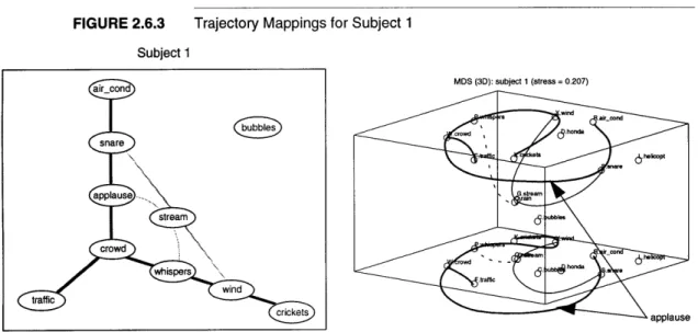
Trajectory Mappings for Subject 1... 42
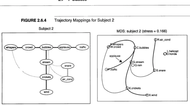
Trajectory Mappings for Subject 2... 43
P-classes by Kind of Source... ... 44
P-classes by Sound Characteristics ... 45
Transitions of Features ... 47
Example of a Time-Frequency Representation: a Constant-Q Transform... 48
A Variety of Sound Representations ... 49
Filterbank R esponse ... 51
O riginal Signal ... 52
Imaginary Part of the Hilbert Transform... 52
Magnitude of the Hilbert Transform (Energy Envelope)... 53
Phase of the Hilbert Transform... 53
Example of Distributions of Atoms: the Copier... 54
Transitions for a Sine Wave ... 57
Cluster Approximation of the Transitions of a Sine Wave... 58
Example of a 2-D Conditioning Neighborhood... 60
Spectrogram of "airplane"... 66 Spectrogram of "aircond" ... 66 Spectrogram of "applause_08" ... ... 66 Spectrogram of "bubbles"... 67 Spectrogram of "crickets"... ... 67 Spectrogram of "crowd_02" ... 67 Spectrogram of "crowd_06" ... 67 Spectrogram of "helicopt" ... ... ... 68 Spectrogram of "honda... 68 Spectrogram of "rain " ... 68 Spectrogram of "snare"... 68 Spectrogram of "stream "... 69 Spectrogram of "traffic"... ... ... 69 Spectrogram of "whispers" ... ... ... 69 Spectrogram of "w ind" ... 69
FIGURE 4.2.1 FIGURE 4.2.2
FIGURE 4.2.3
FIGURE 5.1.1 FIGURE 5.4.1
Computed Distances Between the Textures of Training Set... 72
MDS of Distances Computed with 64 Clusters ... 73
Dissimilarities Measured from Test Set to Training Set (64 and 256 Clusters)... 75
Clicks, Harmonic Components and Noise Patches on a Spectrogram... 79
List of Tables
TABLE 2.1.1 TABLE 2.1.2 TABLE 2.1.3 TABLE 2.1.4 TABLE 2.4.1 TABLE 2.4.2 TABLE 2.4.3 TABLE 2.5.1 TABLE 2.5.2 TABLE 2.6.1 TABLE 2.7.1 TABLE 3.5.1 TABLE 4.1.1 TABLE 4.1.2 TABLE 4.2.1 TABLE 4.2.2 TABLE 4.2.3 TABLE 4.2.4 TABLE 4.2.5Brainstorm: Examples of Sound Textures ... 18
Brainstorm: Sound Texture Characteristics, Qualifiers and Other Determinants... 19
Brainstorm: Properties of Sound Textures... 20
TextureSynth TM Demo Controls... 22
Set of Stimulus for the Similarity Experiment ... ... 29
Similarity Matrix for Subject 1... 29
Final Stress of the MDS Mappings... 32
Set of Stimulus for the First Grouping Experiment... 35
Compilation of the Groupings of Sound Textures Done by the Subjects... 38
Set of Stimulus for the Ordering Experiment ... 41
Selected P -classes ... 43
Notation for a Time-Frequency Feature Space... 60
Set of Signals Used for Analysis and Classification... 65
Time and Frequency Offsets for the Neighborhood Mask ... 70
Dissimilarities between the Textures of the Training Set with 256 Clusters ... 72
Dissimilarities Measured from Test Set to Training Set for 8 Clusters ... 74
Dissimilarities Measured from Test Set to Training Set for 64 Clusters ... . ... 74
Selected P -classes ... 75
Chapter 1 Introduction
This thesis is about human perception and machine classification of sound textures. We define a sound texture as an acoustic signal char-acterized by its collective long-term properties. Some examples of sound textures are: copy machine, fish tank bubbling, waterfall, fans, wind, waves, rain, applause, etc.
1.1 Motivation
Sound textures are an interesting class of sounds, yet different from the other classes of sound studied by most researchers. Contrary to speech or music, sound textures do not carry a "message" which can be decoded. They are part of the sonic environment: people will usu-ally identify them and extract relevant information (their meaning in the current context) and then forget about them as long as the sonic environment does not change.
There currently exists no meaningful way to describe a sound texture to someone other than have them listen to it. The vocabulary to qualify sound textures is imprecise and insufficient, so humans tend to identify them by comparison to a known sound source ("it sounds like a motor, like a fan, like a group of people"). This method of qualification does not transpose easily to machine classification.
Some current models for analysis of sounds by machine extract features like harmonics that occur in a deterministic fashion: the sound is defined as the specific features in the specific order. These models are too rigid for sounds that are stochastic in nature, sounds
1.2 Overview
that have no definite start or end. There are other deterministic anal-ysis methods like embedding, stochastic methods like Markov mod-els, models that assume sound is filtered white noise, and so on. These methods are not well suited for analysis of sound textures.
Our analysis of sound textures assumes that sounds are made up of sound atoms (features) that occur according to a probabilistic rule. Under this assumption, analysis involves extracting the sound atoms and building a probabilistic model. These probability models are high-order statistics, and classification with those models is not a trivial task. Feature selection is an important part of the design of the analyzer; sound atoms should carry perceptual meaning and should aggregate data to reduce the complexity of the probabilistic model.
We devised some psycho-acoustic experiments to find out into which classes people sort sound textures. We will later compare human classification with machine classification.
1.2 Overview
Chapter two summarizes what we found about human perception of sound textures. Chapter three explains the machine classification scheme. Chapter four gives results for machine classification. Chap-ter five suggests some areas of further research in sound textures.
Our work with human perception of sound textures was roughly divided in two parts: first an informal part with small "focus groups", then some more formal psycho-acoustic experiments. We formed small focus groups to come up with examples, qualifiers, classes, perceived parameters and properties of sound textures. We did brainstorms, group discussions and listening sessions. Then we ran three psycho-acoustic experiments: a similarity experiment to see which sounds are perceived similar to each other, a classifying exper-iment to find preferred groupings of sound textures, and an ordering experiment to find the relations between textures. Finally, classes of textures that are considered to belong together by most subjects are formed using the groupings observed in the experiments. We call those human classifications P-classes to distinguish them from the machine classifications to be presented later. Each P-class has a name that should be indicative enough that most subjects would make the same groupings when given only the P-class name and a set of uni-dentified textures.
The machine analysis system first extracts sound atoms from tex-tures, and then builds a probabilistic model of the transitions of atoms. Atom selection is critical: atoms must be perceptually salient features of the sound, but they must not make too strong assump-tions about the kind of sound at the input. The system currently uses points of the magnitude of a spectrogram as sound atoms. Vectors
1.3 Background
containing observed transitions of the parameters of atoms are then formed, and these transition vectors are clustered to extract the most likely transitions. Classification is done by comparing the likely tran-sitions of unknown textures with the trantran-sitions stored in templates. The templates are formed by analyzing typical textures from one P-class.
Samples from twelve textures are used to train the machine clas-sifier. Each sample is assigned one or more of the six P-classes labels: periodic, random, smooth-noise, machine, water and voices. Fifteen samples are used to test the classifier, twelve of which are taken from different segment of the textures used for training, and three samples from new textures. The dissimilarity measure is consistent for differ-ent samples of the same texture. The classifier clearly discriminates its training textures. For the testing set used, the classification done
by machine was the same as the classification into P-classes in more
than 85% of the cases.
1.3 Background
The first concept in our planned work is modeling a complex signal using a representation that addresses the underlying cognitive struc-ture of the signal rather than a particular instance of the signal. A lot of work has been done on modeling, most of which assumes some knowledge of the signal source. Examples of physical modeling of sound sources can be found in [SCH83], [SM183], [SM186] and
[GAR94].
The probabilistic model used in this thesis does not assume such knowledge about the source, at least at a high level; it can encode arbitrary transitions of any features of a signal. It does assume sta-tionarity of the signal in a probabilistic sense, which we equate to the perceptual similarity of any time portion of the texture. With our proposed method the (physical) modeling is replaced by a high-dimensional probability density estimation. This is a newer field, but some of the groundwork has been done [SC083][SIL86]. For the probabilistic modeling, we will use the work of Popat and Picard [POP93] as a starting point.
Sound textures are not new, but they have received less attention than other classes of sounds, for example timbres. In fact, most stud-ies treat sounds as specific events limited in time, not as textures. One problem with researching sound textures is that they are refer-enced under many other names. Our library search for related work in the library has met with very little success.
Feature selection for sound is a very wide topic, which can be (and has been) the subject of countless theses. The human cochlea is known to do a log-frequency decomposition [RIC88], p.312
1.4 Applications
and [M0092]. This provides a good starting point for feature selec-tion, given what is known now. We will explore a few alternatives, like simple forms of filtering [VA193] for preprocessing the sampled (PCM) signal.
Using a high-level model to characterize the transitions of low-level features in sound is not entirely new; it has been done to some extent for breaking, bouncing and spilling sounds [GAV94][WAR84]
Connection to Other Groups at the Media Lab
The cluster-based probability model used for machine analysis was developed at the Media Lab by Picard and Popat of the Vision and Modeling group. It has been used to classify and resynthesize visual textures. The cluster-based probability model has also been shortly
explored for modeling timbres by Eric Metois (music
group) [MET94].
Whitman Richards developed the Trajectory Mapping (TM) tech-nique, and used it to show paths between visual textures. Stephen Gilbert used TM on musical intervals. Whitman Richards expressed interest in mapping from visual textures to sound textures [RIC88]. Michael Hawley has addressed the problem of classification of sounds in his Ph. D. Thesis [HAW93].
In the Machine Listening group, Dan Ellis worked intensively on extracting low-level features from sounds and grouping them [ELL94]. Michael Casey works on physical modeling for sound production [CAS94]. Eric Scheirer has done some work on probabi-listic modelling of transitions of musical symbols.
1.4 Applications
Sound texture identification is an important cue for the awareness of the environment. Humans and animals constantly listen to the ambi-ent texture and compare with similar textures previously experi-enced. Sound textures can have a strong impact on the emotions of the listener (e.g. fear) and can also influence their actions (the sound of rain prompts to avoid getting wet, the sound of voices to prepare for social contact...)
Similarly, machines can get information about the environment
by listening to sound textures. Autonomous creatures (real or
vir-tual) can use this information to direct their actions.
Successful models for machine representation and classification of sound textures could help us understand how humans perceive and classify a wide range of complex, changing sounds.
1.5 Summary of Results
Sound textures are almost always present in movies, in one form or another. This makes sound texture identification a privileged tool in sound track annotation. The sound texture classifier might also be trained to recognize the presence of other classes of signal, and signal other systems to start acting: for example the detection of speech may be made to trigger a speech recognizer and a face recognition
pro-gram.
An optimal method for analysis of a sound texture should pro-duce a representation that is small compared to the original sampled sound. Furthermore, the extracted model can be used to generate new textures of indefinite length. This points to very efficient com-pression. Just as speech can be compressed to the text and music to a MIDI stream, ambiance could be compressed to a compact representation [GAR94].
Creating and modifying sound textures would be of use for sound track ambiance creation, or virtual environments. Addition of a surrounding sound ambiance could add information to a user interface in a non-monotonous way. The ability to modify a texture using semantic parameters greatly increases the usability of the tex-ture editor. Interpolation between two or more textex-tures could pro-duce new textures that combine some of the perceived meaning of the original textures, possibly in an unnatural but interesting fashion (e.g. a voice engine: voice phonemes with an engine-like high-level structure).
1.5 Summary of Results
Human Perception We performed some perception experiments which show that people can compare sound textures, although they lack the vocabulary to ex-press formally their perception.
We have also seen that the subjects share some groupings of sound textures. There seem to be two major ways used to discrimi-nate and group textures: the characteristics of the sound (e.g. peri-odic, random, smooth) and the assumed source of the sound (e.g. voices, water, machine).
Machine Classification The machine classifier we implemented is able to accurately identify samples of the same sound texture for more that 85% of the samples. The dissimilarity measure is smaller between periodic sounds, and between random sounds, which agrees with human perception of similarity. Frequency content of the samples also has an influence on classification.
Chapter 2 Human Perception of Sound Textures
Chapter Overview In the first section of this chapter we summarize our early efforts at collecting examples of Sound Textures and finding their perceived qualifiers and parameters. We proceed to propose a definition of sound textures to be used in the scope of this work. Section 2.3 intro-duces the three psychoacoustic experiments on similarity (§ 2.4), grouping (§ 2.5) and ordering (§ 2.6) of Sound Textures, and report
findings. Finally, we present a simple set of classes for Sound Tex-tures based on the human experiments, which we call P-classes.
2.1 What do You Think is a Sound Texture?
The first logical step in our research on Sound Textures was to find out how people would characterize and define them. For this we had many informal meetings with "focus groups" of four to six people of different background, where we would brainstorm about sound tex-tures, make several listening tests, discuss and record the interven-tions. The concept of a sound texture was at first very difficult to pin down, and discussing in groups brought many simultaneous points of view on the subject. One of the first suggestions was to look in the dictionary.
2.1 What do You Think is a Sound Texture?
Dictionary Definition
TABLE 2.1.1
The on-line Webster dictionary has many interesting definitions for texture:
0 la: something composed of closely interwoven elements
0 1b: the structure formed by the threads of a fabric
* 2b: identifying quality: CHARACTER
* 3: the disposition or manner of union of the particles of a body or substance
* 4a: basic scheme or structure: FABRIC * 4b: overall structure: BODY
From definitions la and 3, we could propose that sound textures are composed of closely interwoven sound particles. Definition lb and 4 suggests the existence of a structure. Definition 2b suggests that the texture helps to identify a sound. These pointers are surpris-ingly adequate for a lot of our work on sound textures. In fact, the three themes (sound particles, structure, identification) are key con-cepts in this thesis.
On the first meeting the groups were asked to give examples of sound textures. The format was a brainstorm, where the ideas were written down on the board, and discussion was not allowed at first, to let every one speak with spontaneity. On a second pass, some of the sounds were rejected from the "Texture" list, and some other items were added to the "Not a Texture" list. Table 2.1.1 is a compila-tion of results.
Brainstorm: Examples of Sound Textures
Texture Not a Texture
rain running water one voice
voices whisper telephone ring
fan jungle music
traffic crickets radio station
waves ice skating single laugh
wind city ambiance single hand clap
hum bar, cocktail sine wave
refrigerator amplifier hum
engine 60 Hz
radio static coffee grinder
laugh track (in TV show) bubbles
applause fire
electric crackle whispers
babble snare drum roll
murmur heart beat
Chapter 2 Human Perception of Sound Textures 18 2.1.1 Examples
2.1 What do You Think is a Sound Texture?
Texture or Not? One very dynamic activity of the focus groups was an informal ex-periment where the author would play a lot of different sounds and ask the group whether each can be called a texture. This experiment was very important in showing that each person has specific criteria of what is a texture, and those criteria can vary quite a lot from one person to the other.
2.1.2 Perceived Characteristics and Parameters
The groups were then asked to come up with possible characteristics and qualifiers of sound textures, and properties that determine if a sound can be called a texture. Sorting the answers produced the fol-lowing tables, split into a few loose conceptual classes: characteris-tics, qualifiers, other determinants and properties. Characteristics (usually nouns) apply to all textures to some degree; Qualifiers (usu-ally adjectives) may or may not apply at a certain degree to each tex-ture; Other Determinants have a strong impact on how the sound is produced or perceived; Properties are required of all sound textures. Table 2.1.2 show the first three lists. Lists can overlap: for example, the characteristic randomness can be seen as an axis, and the qualifier random points to the high end of that axis.
TABLE 2.1.2 Brainstorm: Sound Texture Characteristics, Qualifiers and Other Determinants
Characteristic Qualifier Other Determinant
volume loud is machine spectrum content
randomness repetitive pitched "tone color"
regularity random noisy granular shape
periodicity voiced environmental "could be produced with
frequency chaotic ambient this model"
smoothness steady periodic
irritability dangerous harsh
grain size quiet human
time scale pleasant granular
period length is voice rhythmic
brightness rough smooth
density man-made discrete
complexity natural continuous
contrast is water "has sharp onsets"
spaciousness annoying violent
size of source energy force
There is obviously a lot of overlap within the Characteristics, and also between the Qualifiers and Characteristics. If we consider Char-acteristic to be akin to axes of the texture space, they could hardly form an orthogonal basis. Furthermore a lot of them are highly sub-jective, which removes even more of their usability as a basis.
2.1 What do You Think is a Sound Texture?
Properties
TABLE 2.1.3
Parallel with Visual Texture Parameters
A few of the more subjective characteristics and qualifiers are
specially interesting. "Annoying" is a qualifier that surfaced often when participants were listening to recorded textures; it was often associated with a strong periodicity, a sharp volume contrast, and the presence of high frequencies. However, sounds qualified "annoying" could have all kinds of other qualifiers; they were not confined to a specific sub-space of the Characteristic "axes" either. Similar remarks could be made about most of the other subjective qualifiers: environ-mental, pleasant, violent, natural, etc.
Another preeminent qualifier is the sensation of danger. It was often associated with a large estimated source size, which in turn was associated with the presence of low frequencies. Listeners were rather unanimous in their evaluation of what textures sounded dan-gerous (more unanimous than for almost all other appreciations on sound textures). The "danger" sensation from sound seems to be wired in the human brain, as it is probably for all animals with hear-ing capabilities.
This brings us to a very important observation: sound textures
carry a lot of emotion. With the exception of smell, they are probably
the strongest carrier of emotions for human beings; even in speech or music the emotional content is not so much dependant on words or melodies but to a great extent on a "mood" more linked to the "tex-tural" aspect than the semantics.
A few properties were mentioned as essential for a sound to be a
tex-ture; they are summarized in Table 2.1.3. They will be used to form a working definition of sound textures in Section 2.2.
Brainstorm: Properties of Sound Textures
cannot have a strong semantic content
"ergodicity": perceptual similarity of any (long enough) segment in time
long time duration
Some of the perceived characteristics of sound textures have obvious parallels in visual textures: periodicity and period length, complexi-ty, randomness, granular shape, and "could be produced with this model". Sound volume can be associated with visual intensity, and visual contrast with volume contrast. Color is in some ways similar to sound frequency content (sometimes referred to as tone color). Vi-sual orientation is difficult to equate with a sound characteristic, al-though some sounds are characterized by a shift in frequency content with time. In a fishtank bubble texture, for example, each bubble starts with a low frequency moving upwards (see Figure 4.1.4), so that upwards or downwards movement in frequency could be asso-ciated with visual orientation, although this effect in sound is less im-portant than in vision.
2.1 What do You Think is a Sound Texture?
Even some of the more subjective qualifiers, like natural, annoy-ing, man-made and annoying have parallels in the visual domain.
In the course of our texture exploration, we also experimented with two pieces of Macintosh software for synthesizing visual tex-tures. The first KPT Texture Explorer TM obviously has some internal
model of visual textures, with an unknown number of parameters, but the user controls are very limited: at any point one can only choose only one of 12 textures shown, choose a mutation level, and initiate a mutation which produces 12 "new" textures. There is also a control for mutating color. Despite the poorness of the controls, the program includes a good selection of seed textures, which helps to get visually interesting textures.
The second program, TextureSynth TM Demo, is more interesting
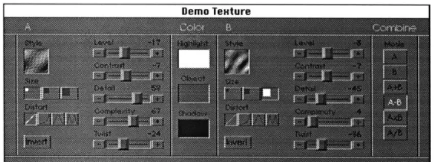
in the way it lets users modify textures. It offers 12 controls, described on Table 2.1.4. The control window has two sets of 9 con-trols (sliders, buttons and pop-up menus) to produce two textures (A and B) which are then combined (A,B, A+B, A-B, AxB, A--B). The results are visually interesting, and the controls are usable. Still, it is obvious that modifying textures is a difficult problem, both from the synthesis model point of view and the user control point of view.
FIGURE 2.1.1 TextureSynth TM Demo Control Window
2.1 What do You Think is a Sound Texture?
There are many parallels between the controls in TextureSynth TM Demo and possible parameters of sound textures. The last column of Table 2.1.4 points to some possible choices.
TABLE 2.1.4 TextureSynth TM
Demo Controls
Name Type Description Parallel with Sound Textures
Style popup: 8 choices basic style: plaster, waves, fiber, basic class: machine, voices, rain,
plaid, etc. etc.
Size buttons: 3 choices fine, medium or coarse grain time scale
Distort buttons: 3 choices lookup table from function intensity
-Invert on/off button reverses intensity scale
-Level slider mid-point of intensity volume
Contrast slider dynamic range of intensity volume contrast
Detail slider low/high frequency ratio number of harmonics,
low/high frequency ratio
Complexity slider randomness randomness
Twist slider orientation
Shadow popup: 25 choices color mapped to low intensity
Object popup: 25 choices color mapped to medium intensity Frequency contents
Highlight popup: 25 choices color mapped to high intensity
2.1.3 Classes and Categories
The participants in one focus group had many reservations about whether it was possible, or even desirable, to come up with classes or categories of sound textures. One foreseen difficulty was that there are many possible kinds of classes:
* by meaning
* by generation model - by sound characteristics
Also, people had great difficulties in coming up with names for categories without first having an explicit set of textures to work with. This would support views that for one class of signals, people use many different models and sets of parameters, and that identifi-cation is context-dependent.
Because of those difficulties, we decided to do classification experiments in which a set of sound textures are provided; this is described in the rest of this chapter. The first obvious problem was to try to collect a set of textures that would well represent the space of all possible textures. It is not possible to do an exhaustive search of this infinitely complex space, so we tried to collect as many examples as possible and then limit the redundancy. The examples were taken
2.2 Working Definition of Sound Textures
by asking many people, by recording ambient sounds, and by
search-ing databases of sounds. Still, any collection of sound textures is bound to be incomplete.
2.2 Working Definition of Sound Textures
Too Many Definitions During the focus group meetings, it quickly became obvious that there are many definitions of a sound texture, depending on whom you ask. However, most people agreed on a middling definition which included some repetitiveness over time, and the absence of a complex message.
John Stautner suggests that textures are made of "many distin-guishing features, none of which draws attention to itself. A texture is made of individual events (similar or different) occurring at a rate lower than fusion; using an analysis window, we can define a texture as having the same statistics as the window is moved." [STA95]
This would seem a reasonable definition, but it is made difficult because it depends on many variable concepts: "distinguishing", "drawing attention", fusion rate, window size, etc. The concepts of "distinguishing" and "drawing attention" are totally subjective. The acceptable range for fusion rate and window size are once again vari-able.
When asked to draw the boundary for fusion, participants in the focus groups all agreed that the rate was lower than 30Hz. As for the window size, the upper boundary was limited by an "attention span" of a few (1-5) seconds, with the argument that events too far apart are heard as independent of each other.
2.2.1 Working Definition of Sound Texture
A natural step at this point was to refine a definition for Sound
Tex-ture to be used in the scope of this work.
Defining "Sound Texture" is no easy task. Most people will agree that the noise of fan is a likely "sound texture". Some other people would say that a fan is too bland, that it is only a noise. The sound of rain, or of a crowd are perhaps better textures. But few will say that one voice makes a texture (except maybe high-rate Chinese speech for someone who does not speak Chinese).
2.2 Working Definition of Sound Textures
First Time Constraint: Constant Long-term Characteristics
A definition for a sound texture could be quite wide, but we chose to
restrict our working definition for many perceptual and conceptual reasons. First of all, there is no consensus among people as to what a sound texture might be; and more people will accept sounds that fit a more restrictive definition.
The first constraint we put on our definition of a sound textures is that it should exhibit similar characteristics over time; that is, a two-second snippet of a texture should not differ significantly from another two-second snippet. To use another metaphor, one could say that any two snippets of a sound texture seem to be cut from the same rug [RIC79]. A sound texture is like wallpaper: it can have local structure and randomness, but the characteristics of the structure and randomness must remain constant on the large scale.
This means that the pitch should not change like in a racing car, the rhythm should not increase or decrease, etc. This constraint also means that sounds in which the attack plays a great part (like many timbres) cannot be sound textures. A sound texture is characterized
by its sustain.
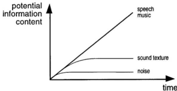
Figure 2.2.1 shows an interesting way of segregating sound tex-tures from other sounds, by showing how the "potential information content" increases with time. "Information" is taken here in the cog-nitive sense rather then the information theory sense. Speech or music can provide new information at any time, and their "potential information content" is shown here as a continuously increasing function of time. Textures, on the other hand, have constant long term characteristics, which translates into a flattening of the potential information increase. Noise (in the auditory cognitive sense) has somewhat less information than textures.
FIGURE 2.2.1 Potential Information Content of A Sound Texture vs. Time
potential speech information music content sound texture noise time
Sounds that carry a lot of meaning are usually perceived as a message. The semantics take the foremost position in the cognition, downplaying the characteristics of the sound proper. We choose to work with sounds which are not primarily perceived as a message.
2.2 Working Definition of Sound Textures
Note that the first time constraint about the required uniformity of high level characteristics over long times precludes any lengthy mes-sage.
Two-level Representation
Sounds can be broken down into many levels, from a very fine (local in time) to a broad view, passing through many groupings suggested
by physical, physiological and semantic properties of sound. We
choose, however, to work with only two levels: a low level of simple atomic elements distributed in time, and a high level describing the distribution in time of the atomic elements.
We will bring more justification for this choice in Chapter 3, when we talk about our definition of sound textures for machine pro-cessing.
Second Time Constraint: Attention Span
The sound of cars passing in the street brings an interesting problem: if there is a lot of traffic, people will say it is a texture, while if cars are sparse, the sound of each one is perceived as a separate event. We call "attention span" the maximum time between events before they become distinct. A few seconds is a reasonable value for the attention span.
We therefore put a second time constraint on sound textures: high-level characteristics must be exposed or exemplified (in the case of stochastic distributions) within the attention span of a few sec-onds.
This constraint also has a good computational effect: it makes it easier to collect enough data to characterize the texture. By contrast, if a sound has a cycle of one minute, several minutes of that sound are required to collect a significant training set. This would translate into a lot of machine storage, and a lot of computation.
Summary of our * Our sound textures are formed of basic sound elements, or
Working Definition atoms;
* atoms occur according to a higher-level pattern, that can be periodic or random, or both;
* the high-level characteristics must remain the same over long time periods (which implies that there can be no complex message);
* the high-level pattern must be completely exposed within a few seconds ("attention span");
e high level randomness is also acceptable, as long as there are enough occurrences within the attention span to make a good example of the random properties.
2.3 Experiments with Human Subjects
2.3 Experiments with Human Subjects
We conducted three sound texture classification experiments, each with 4-8 subjects. The experiments were approved by the MIT Com-mittee on the Use of Human Experiment Subject (COUHES, request 2258).
Goal
In doing experiments with human subjects, we want to confront the subjects with actual sound textures and explore their reactions. We first want to see what kind of parameters are actually used by naive subjects to sort the sound textures. The second important goal is to find the kinds of groupings that subjects make, and how they "label" these groupings. This last information was then used to build P-Classes, which are the subject of a further section.
2.3.1 Common Protocol
The interface is based on the Macintosh finder, without any special programming. Sound textures are each identified with an icon, and can be played (double-click), moved (drag) and copied (option-drag). Each experiment trial is self-contained in a window, with the re-quired texture icons in the right place. Special care is taken to insure that windows show up on the right place on the screen, and don't overlap.
The sounds are played by SoundApp (Freeware by Norman Franke). The stimuli were taken from the Speed of Sound sound effect compact disk.
Shortcomings Using the Finder greatly reduces the time required to set the experi-ments up, but it also reduces the flexibility of the system as com-pared to programmed systems. The main drawbacks are:
* the data is not automatically collected in machine form, - copying texture icons can be awkward, and
* playback cannot be robustly interrupted.
2.4 Similarity Experiment
Goal
In the first experiment we measure the perception of similarity be-tween sound textures and form a map where the distance bebe-tween any two textures is roughly inversely proportional their similarity. The resulting map should bring together the textures which are per-ceived similar, if it is possible on a two-dimensional map. Because
MDS is an optimization procedure that tries to achieve a best fit, the
distance on the map may not always reflect the perceived similarity.
2.4 Similarity Experiment
2.4.1 Method: Multidimensional Scaling (MDS)
Multidimensional Scaling is a well-known method to build a low-di-mensional map of the perceived distances between a set of stimuli
[JOH82]. It is based on an iterative algorithm to optimize the relative
position of the stimuli on the map to match to the perceived similari-ties or dissimilarisimilari-ties.
In our experiment, we collect rank-ordered perceived similarities (as opposed to perceived distances). For example, with a set of 12 tex-tures, we give a similarity rank of 11 to the texture perceived the clos-est to the reference texture, then a 10 for the next closclos-est, and so on until the subject thought the remaining textures are perceived as not similar (rank 0). This measure of perceived similarity is valid for ordering but should not be taken as an absolute measurement.
These similarities are successively collected with each texture as a reference to form a similarity matrix. The similarity matrix is then fed to the well known Kyst2a program from AT&T [KRU77]. The data is specified to be non-metric similarities. We request a two-dimensional map, so Kyst produces a set of (x,y) coordinates for each texture.
Protocol
In this experiment, the subject is presented with a small set of sound textures which remains the same throughout all the trials of the ex-periment. As a trial begins, a reference texture is played and the sub-ject must try to find the most similar texture in the rest of the set. The subject then looks for the next texture most similar to the reference texture and so on, until it is felt that the remaining textures are com-pletely different from the reference texture.
2.4 Similarity Experiment
Trial Window for the Similarity Experiment
I2iems 1,899.1 MBin disk 137.3MB~aale
AIFF AIFF
SAiWt AIFF Da
AIFF
AIFF
AIFF Xik, AIFF
AIFF AIFF AIFF fA Rawt AF reference texture space available for manipula-tion of icons
There are as many trials as there are sounds in the set, so the sub-ject gets to match each texture. There is a different window for each trial, and each window contains icons for all the sounds from the set, in random positions. Each icon is identified by a capital letter. These letters have no meaning, they are for identification only. The icon for the reference texture is always in the lower left corner of the window, and the others at the top of the window (see Figure 2.4.1). The subject listens to a sound by double-clicking on its icon, and can stop the playback by typing a dot (".") before clicking on anything else. A data sheet is provided to note the results at the end of each set. The icons can be moved around the window to help organize the sounds; only the data sheet is used to collect results, not the final window configuration.
The set contains the 12 textures shown on Table 2.4.1. The signals were scaled to have a maximum dynamic range, but the loudness perception varied. The sound textures are each identified by a
ran-Chapter 2 Human Perception of Sound Textures 28 FIGURE 2.4.1
2.4 Similarity Experiment
TABLE 2.4.1
2.4.2 Results
dom capital consonant. The experiment took an average of 35 min-utes to complete.
Set of Stimulus for the Similarity Experiment
identifier name description
C bubbles fish tank bubbles
D honda idling motorcycle
F traffic many individual traffic horns
G stream quiet water stream or brook
K crickets constant drone of many crickets outside
L helicopt closed-miked constant helicopter rotor
P whispers many people whispering, with reverb
Q rain constant heavy rain
R aircond air conditioning compressor & fan
S snare constant snare drum roll
W crowd medium-sized crowd inside, with reverb
X wind constant wind outside
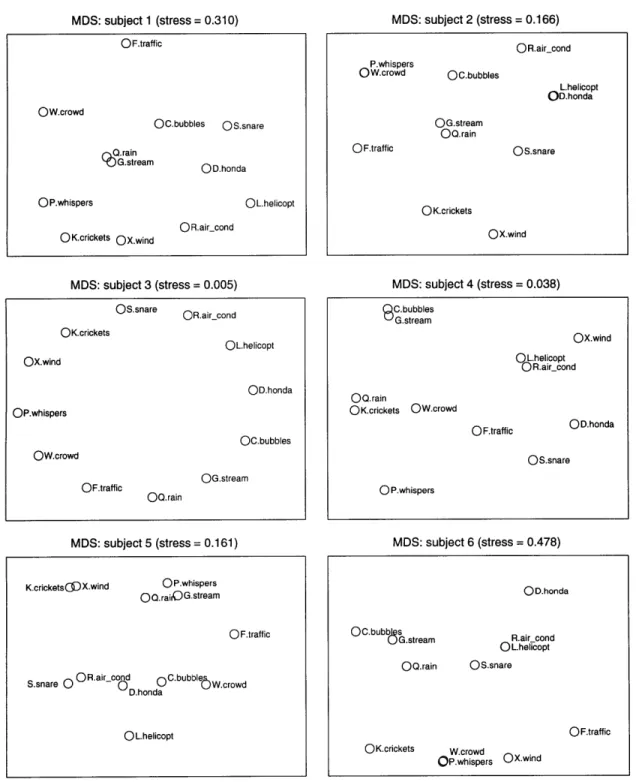
The similarity perception data was collected from the trials into a similarity matrix, as in Table 2.4.2. To visualize the data, MDS maps are formed using the kyst algorithm. The two dimensional maps are shown on Figure 2.4.2.
Similarity Matrix for Subject 1
For all six subjects, four sounds (helicopter, air conditioning, motorcycle and snare) formed a localized group, with no other sound mixed in. Four subjects brought bubbles close to that latter group. The three sounds produced by water (bubbles, stream and rain) were also in a loose local group for all six subjects. Subjects 2 and 6 gave a high similarity to whispers and crowd, and three other subjects
con-Chapter 2 Human Perception of Sound Textures 29 TABLE 2.4.2
2.4 Similarity Experiment
FIGURE 2.4.2 Individual MDS Results
MDS: subject 1 (stress = 0.310) 0 F.traffic OW.crowd OC.bubbles OS.snare 9 Q.rain G.stream OD.honda OP.whispers OL.helicopt
OK.crickets OX.wind OR.air-cond
MDS: subject 3 (stress = 0.005)
Os.snare OR.air cond OK.crickets OL.helicopt OX.wind OD.honda OP.whispers OC.bubbles OW.crowd OF.traffic . G.stream QQ.rain MDS: subject 5 (stress = 0.161) (Subjects 1, 2, 3, 4, 5 and 6) MDS: subject 2 (stress = 0.166) OR.airscond P.whispers OW.crowd OC.bubbles L.helicopt OD.honda OG.stream OQ.rain OF.traffic OS.snare OK.crickets OX.wind MDS: subject 4 (stress = 0.038) C.bubbles G.stream OX.wind o L.helicopt O R.aircond
OQ.rain
OK.crickets OW.crowd OF.traffic OD.honda OS.snare O P.whispers MDS: subject 6 (stress = 0.478) K.crickets(3)X.wind OP.whispers OQ.raiOG.stream 0 F.traff icS.snare 0 O R.air cod 0 C.bubble Wd D.honda
OL.helicopt
Chapter 2 Human Perception of Sound Textures 30
OD.honda
QC.bubb~a
uG.stream R.air cond
OL.helicopt
OQ.rain Os.snare
OF.traffic
OK.crickets W.crowd
2.4 Similarity Experiment
sidered them rather similar. Four people considered crickets and wind similar. Crowd is a neighbor to traffic in five of the MDS results.
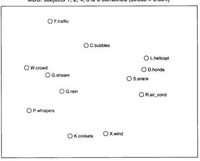
Not surprisingly these observations apply to the MDS analysis of the combined data, shown on Figure 2.4.3. Note that the data for sub-ject 3 was not included because the experiment protocol was not
fol-lowed as closely in that case, as discussed in the next paragraph.
FIGURE 2.4.3 Combined MDS Results for Subjects 1, 2, 4, 5 & 6
MDS: subjects 1, 2, 4, 5 & 6 combined (stress = 0.394)
0 F.traffic 0 c.bubbles 0 W.crowd 0 G.stream 0 Q.rain
o
L.helicopt 0 D.honda 0 S.snare 0 R.air-cond 0 P.whispers 0 K.crickets 0 X.windMDS in an approximation procedure which minimizes a
mea-sure of stress. In this case, the stress indicates the deviation of the dis-tances on the map from the disdis-tances computed from the input data. Because the input data has many more points than there are dimen-sions in the mapping space, the stress for the final map will not be zero. The final stress for the MDS maps are indicated at the top of the figures. They range from 0.005 to 0.478. A map with stress below 0.1 is considered to be a good fit, so only subjects 3 and 4 meet that crite-rion. Subjects 2 and 5 have a slightly higher but acceptable fit. Sub-jects 1 and 6 have a high stress which indicates an improper fit. In those cases, increasing the dimensionality of the mapping space can
2.4 Similarity Experiment
help produce a better fit. Table 2.4.3 shows the final stress for 2- and 3-dimensional mapping of the subject data.
Final Stress of the MDS Mappings
final stress subject 2-D 3-D 1 0.310 0.207 2 0.166 0.100 3 0.005 0.010 4 0.038 0.006 5 0.161 0.102 6 0.478 0.398 subjects 1, 2, 4, 5 & 6 0.394 0.264 combined
In general, the final stress is reduced by mapping onto three dimensions, but not enough to match our criterion for a "good" fit (stress<0.1) in the difficult cases (subjects 1, 6 and combined map). This may indicate that the data for subjects 1 and 6 is less consistent across trials. It is expected that the final stress for combined map is higher because the combination is bound to introduce variance and possibly inconsistencies. Figure 2.4.4 shows 3-dimensional MDS map-pings for subjects 1 and 6; Figure 2.4.5 shows such a mapping for the com-bined data. The plots show a perspective view of the points in 3-D space, as well as a projection of the points on the (x,y) plane.
Three-Dimensional MDS Mappings (subjects 1 and 6) MDS (3D): subject 1 (stress = 0.207) whisp -s qair_cond crickets helicpt sna ..re .whispers (Icrikes Y.crowd ,5traffic ubbles J.aircon .hehico ub .ona snare
MDS (3D): subjects 1, 2, 4, 5 & 6 combined (stress = 0.264)
,_whsper wind &crowd 6.crickets I..ircond (8.stream -.crickets 1 psu espers 6rain .crowd stream .6a bubbles
Chapter 2 Human Perception of Sound Textures 32 TABLE 2.4.3
FIGURE 2.4.4
6h .cpt
honda
2.4 Similarity Experiment
FIGURE 2.4.5 Three-Dimensional MDS Mappings (Subjects 1, 2, 4, 5 & 6 Combined)
MDS (3D): subjects 1, 2, 4, 5 & 6 combined (stress = 0.264)
Proof of Principle of the MDS Algorithm
FIGURE 2.4.6
An interesting case should be brought to your attention: Subject 3 first ordered the textures in a circle (Figure 2.4.6, left side), and then used that ordering to rank the similarities. The MDS algorithm ex-tracted exactly the same order (Figure 2.4.6, right side), which shows that it works as expected. Note that the MDS algorithm has a tenden-cy to arrange data points in a circle, which helped conserve the shape.
Proof of Principle of the MDS Algorithm
MDS: subject 3 (stress = 0.005) OS.snare OR.air-cond OK.crickets OL.helicopt Oxwind OD.honda
OP.whispers
Oc.bubbes OW.crowd F.traffic OG.stream OQ.rainChapter 2 Human Perception of Sound Textures 33
1?t,,s1,894. Imai lak 142 2MBable
AIFF AIFF
A
Rd~t AIFF
Pdas
AWY
-
F2.5 Grouping Experiment
2.5 Grouping Experiment
Goal
2.5.1 Protocol
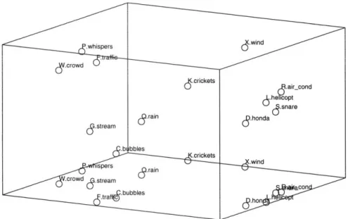
FIGURE 2.5.1
The grouping experiments aimed at discovering what sounds people think go together, and what names they give to the various groups they make. One question of interest was: "Do people group sound textures by their origin, or do they group them by common sound characteristics?".
We hoped to find a common, natural grouping scheme (classes), and later compare the computer classification results with P-classes.
In the grouping experiment, the subject is asked to cluster the tex-tures from a small set into a few groups. The requirements for the clusters are intentionally left vague:
"Cluster the sounds into groups of sounds that you think belong together. Make as many groups as you think are necessary, but not more. Groups can have only one sound, or many."
The subject is presented with a window containing the icons for all the texture in the set (see Figure 2.5.1). The grouping is done by dragging the icons into groups within the window. The window with the clustered icons is then printed, and the subject is asked to give a qualifier to each group. The experiment took an average of 6 minutes to complete, including the printout.
Initial Window for the Grouping Experiment
121ems 1,894.4MBin dik 142MB e
AIFF
Alff - Aly, AIFF
AAIFF CAds AlF
Fahr AlIT
-
Rif,AIFF
AIFF , F
AIFF AF F
01k
2.5 Grouping Experiment
First Grouping Experiment
We did two sets of grouping experiments, with different subjects and slightly different stimulus sets.
A first run of the grouping experiment was done to test the usability
of the interface. The set contained 10 sounds, which were identified with a random mixture of lower and upper case letters, numbers, and symbols (see Table 2.5.1). There were 5 subjects.
TABLE 2.5.1 Set of Stimulus for the First Grouping Experiment identifier name description
* bubbles fish tank bubbles
2 crickets constant drone of many crickets outside
K crowd medium-sized crowd inside, with reverb
% forest constant drone with distant birds
6 helicopter closed-miked constant helicopter rotor
n lawn mower closed-miked constant lawn mower engine
+ rain constant heavy rain
q traffic many individual traffic horns
y transformer strong 60 Hz buzz
F whispers many people whispering, with reverb
Second Grouping Experiment
In the second grouping experiment, the same 12 textures of the simi-larity experiment are used (see Table 2.4.1). The grouping experiment usually immediately follows the similarity experiment, so that the subject has had plenty of opportunity to get familiar with the sounds. There were 7 subjects.
2.5.2 Results
The first grouping experiment showed that subjects quickly accepted the user interface. The icon metaphor was grasped immediately: one icon for each sound texture, double-click the icon to play, drag the icon to organize the groups.
This first experiment also provided a number of groupings, which were in essence similar to those in the second grouping exper-iment; the results are thus combined.
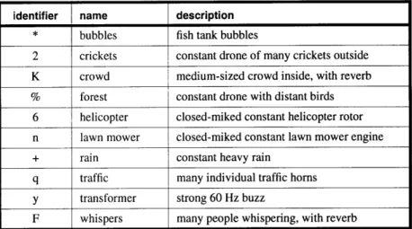
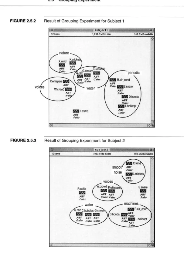
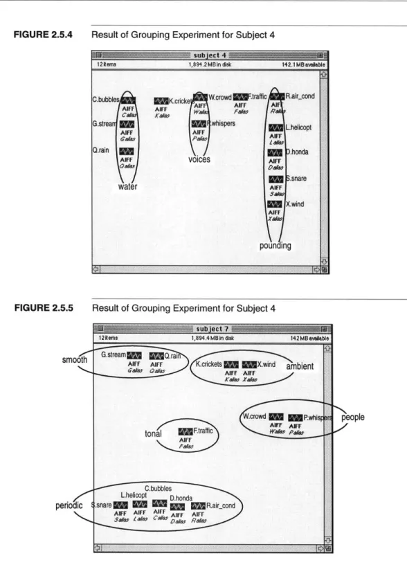
Groupings provided by the subjects are shown on Figures 2.5.2 through 2.5.5. A list of the grouping names and contents is given on Table 2.5.2.
2.5 Grouping Experiment
FIGURE 2.5.2 Result of Grouping Experiment for Subject 1
FIGURE 2.5.3 Result of Grouping Experiment for Subject 2
2.5 Grouping Experiment
FIGURE 2.5.4 Result of Grouping Experiment for Subject 4
12lem 1,8942 MBin dik 4 id
C bubbles K.crcke wdinWtrffic Rair-cond
AlIF AIFF stre whispe s .snare AFF AFT X wlnd AIF poun ing
FIGURE 2.5.5 Result of Grouping Experiment for Subject 4
Chapter 2 Human Perception of Sound Textures
1,894.4MBin disk 142MBOilble
Q~ri
AIrF K.crickets M X.wind ambient
Qafu AIFF AIFF
ats Xa
,crowd P.whisp
AFT AlFF
tonal F.traffic Wa., PAW ,
AIFF
- C.bubbies L.helicopt D honda
M
*3 R.air cond
AFF AlfF AIrF AFF AFF
Sawe ZAi cawt aW RAFF
2.6 Ordering Experiment
The kinds of grouping were quite varied, but some themes occurred more often. It is obvious that the groupings and their names are influenced by the selection of stimuli, but there is no way to avoid that.
Compilation of the Groupings of Sound Textures Done by the Subjects
Subject(s) Group name Group
1,2,3,4,6 water4, watery bubbles, rain, stream
1,2,5,6,7 nature2 crickets, wind
constant, hum smooth, smooth noise "ambient"
1,2,4,6 people2, voices2, crowd, whisper
speechy, spacious
2,3,5 machines3 air_cond, helicopt, honda
1,5 periodic3, mechanical air cond, helicopt, honda, snare
4 pounding air cond, helicopt, honda, snare, wind
7 periodic, hard, close aircond, bubbles, helicopt, honda,
snare
5,7 constant background rain, stream
smooth, random
3 low volume variance crickets, snare, whisper, wind
3 high volume variance crowd, traffic
5 stochastic whispers
5 irregular foreground bubbles, crowd, traffic
7 tonal traffic
2.6 Ordering Experiment
Goal
The third experiment seeks to find how sound textures are related to each other. The Similarity Experiment measured the perceived simi-larities between the sounds to set the distances on a map. On the other hand, the Ordering Experiment tries to find the connections between the textures, like the routes on a subway map.
2.6.1 Method: Trajectory Mapping (TM)
The Ordering Experiment is based on the Trajectory Mapping tech-nique [RIC93]. The subject is presented with all possible pairs of stimuli, and asked to select a feature that changes between the two and then find an interpolator and two extrapolators according to the
Chapter 2 Human Perception of Sound Textures 38 TABLE 2.5.2