An adaptive numeric predictor-corrector guidance algorithm for atmospheric entry vehicles

AN ADAPTIVE NUMERIC PREDICTOR-CORRECTOR GUIDANCE ALGORITHM FOR ATMOSPHERIC

ENTRY VEHICLES

by

Kenneth Milton Spratlin

B.A.E., Georgia Institute of Technology

(1985)

SUBMITTED IN PARTIAL FULFILLMENT OF THE REQUIREMENTS FOR THE DEGREE OF

MASTER OF SCIENCE IN AERONAUTICS AND ASTRONAUTICS

at the

MASSACHUSETTS INSTITUTE OF TECHNOLOGY May 1987

©)Kenneth Milton Spratlin, 1987

Signature

of

Author

..

_ ,

,.

Ad:II

Department bf Aeronautics and Astronautics

May 8, 1987

Approved by .. _ _ ) -j- / ₇

Professor Richard H. Battin Department of Aeronautics and Astronautics Thesis Supervisor Approved by I 'L," I'.LA . -7 I - / -' . ' r ' Tinioth,' J. Brand Technical Supervisor, CSDL Accepted by I, I w I ve v - - vvv I..

V - / Professor Harold Y. Wachman

Chairman, Department Graduate Committee

Archiv es

AN ADAPTIVE NUMERIC PREDICTOR-CORRECTOR GUIDANCE ALGORITHM FOR ATMOSPHERIC

ENTRY VEHICLES

by

Kenneth Milton Spratlin

Submitted to the Department of Aeronautics and Astronautics on May 8, 1987, in partial fulfillment of the

requirements for the Degree of Master of Science in Aeronautics and Astronautics

ABSTRACT

An adaptive numeric predictor-corrector guidance algorithm is developed for atmos-pheric entry vehicles which utilize lift to achieve maximum footprint capability. Applicability

of the guidance design to vehicles with a wide range of performance capabilities is desired

so as to reduce the need for algorithm redesign with each new vehicle. Adaptability is

desired to minimize mission-specific analysis and planning. The guidance algorithm moti-vation and design are presented.

Performance is assessed for application of the algorithm to the NASA Entry Research Vehicle (ERV). The dispersions the guidance must be designed to handle are presented. The achievable operational footprint for expected worst-case dispersions is presented. The algorithm performs excellently for the expected dispersions and captures most of the

achiev-able footprint.

Thesis Supervisor: Dr. Richard H. Battin

Title: Adjunct Professor of Aeronautics and Astronautics

Technical Supervisor: Timothy J. Brand

ACKNO WLEDGEMENT

This report was prepared at The Charles Stark Draper Laboratory, Inc. in support of NASA Langley Research Center (LaRC) Task Order No. 87-43 under Contract NAS9-17560 with the NASA Lyndon B. Johnson Space Center (JSC).

Publication of this report does not constitute approval by the Draper Laboratory or the sponsoring agency of the findings or conclusions contained herein. It is published for the exchange and stimulation of ideas.

I hereby assign my copyright of this thesis to The Charles Stark Draper Laboratory, Inc., Cambridge, Massachusetts.

Kenneth M. Sratlin

Permission is hereby granted by The Charles Stark Draper Laboratory, Inc. to the Mas-sachusetts Institute of Technology to reproduce any or all of this thesis.

I wish to take this opportunity to thank some of the many people who have helped me during the preparation of this thesis and my stay at M.I.T.. I would like to express my sin-cere gratitude to The Charles Stark Draper Laboratory for making my graduate study possi-ble through the Draper Fellowship. I wish to thank all of the members of the Guidance and Navigation Analysis Division for their technical assistance and willingness to share their

expertise. In particular I would like to thank T. Brand, J. Higgins, and A. Engel for their

patience, assistance, and support during the preparation of this thesis and work on the Aeroassist Flight Experiment. I wish to thank my thesis advisor, Dr. R.H. Battin, for his assistance and in particular for his abilities as an educator. A special thanks for his

encour-agement and support goes to B. Kriegsman who recently passed away. He is greatly

missed. I found the opportunity to interact with the people at CSDL to be the most reward-ing aspect of my studies at M.I.T..

I also wish to thank H. Stone and R. Powell of NASA/LaRC for the opportunity to work on the ERV entry guidance problem and their assistance in answering my questions.

Most importantly, I wish to thank my parents and sisters for their unending love and support over the years.

TABLE OF CONTENTS Page Section

... ...

21

3.2 Unit Target Vector .

3.3 Commanded Attitude 3.4 Corrector Algorithm 3.5 Predictor Algorithm 3.5.1 Introduction ... 3.5.2 Equations of Moti( 3.5.3 Integration of the 3.5.4 Termination Cond

3.5.5 Final State Error (

... I... 23

Computation

...

on ...

litions for the Predictor ...

Comnutation

...

3.6 Estimators ...

3.7 Heat Rate Control

...

I

...

48

...

52

4.0 PERFORMANCE ...

4.1 Simulator .-...

4.2 Open-Loop Footprint ...

4.3 Effect of Dispersions on Footprint ...

4.4 Estimator Performance ...

4.5 Closed-Loop Performance ...

4.6 Heat Rate Control Performance ...

4.7 Overcontrol ...

4.8 Algorithm Execution Time ... ...

5.0 FUTURE RESEARCH TOPICS AND

5.1 Future Research Topics ...

CONCLUSIONS . . . . .. . . . 69

...

...

69

Appendix A. ERV AERODYNAMICS MODEL ... 133

Appendix B. ALGORITHM PROGRAM LISTINGS ... 135

List of References ... 211 57 57 57 59 60 61 63 63 66 Appendix

LIST OF ILLUSTRATIONS

Figure Page

1. Three-View Drawing of the ERV ... 78

2. Atmospheric Wind Profile ... 79

3. Envelope of Density Profiles Derived from Shuttle Flights ...- : ... 80

4. STS-1 Density Profile Comparison ... ... 81

5. STS-9 Density Profile Comparison ... 82

6. Multiphase Bank Angle Program for L/D = 1.5 ... ... 83

7. Crossrange Versus Number of Bank Steps ... 84

8. Comparison of Optimum Bank Angle Programs ... 85

9. Optimum Shuttle Angle of Attack Profile for Maximum Downrange ... 86

10. Optimum Shuttle Bank Angle Profile for Maximum Crossrange ... 87

11. Optimum Shuttle Angle of Attack Profile for Maximum Crossrange ... . 88

12. Landing Footprint for the ERV ... 89

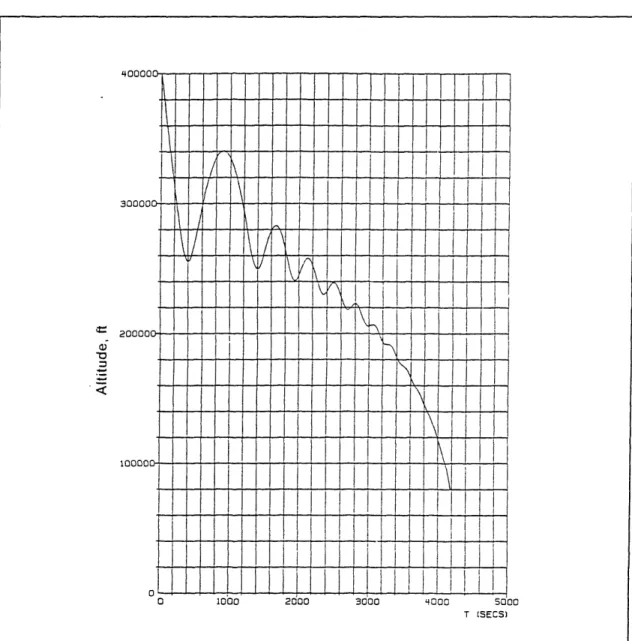
13. Altitude Histories for the Entry Missions of the ERV ... 90

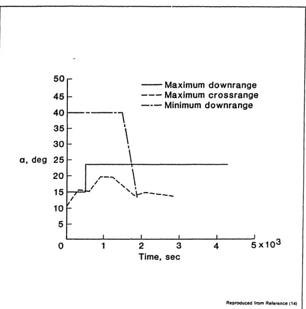
14. Bank Angle Histories for the Entry Missions of the ERV ... 91

15. Angle of Attack Histories for the Entry Missions of the ERV ... 92

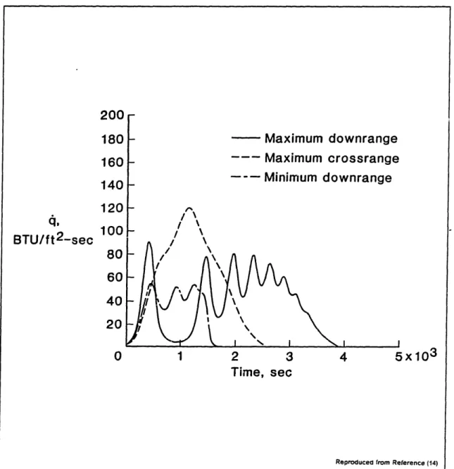
16. Heat Rate Histories for the Entry Missions of the ERV ... 93

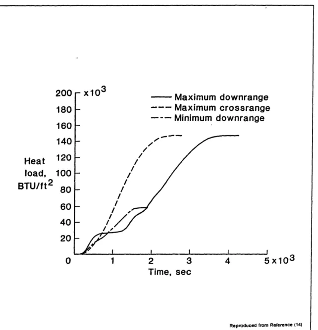
17. Heat Load Histories for the Entry Missions of the ERV ... 94

18. Bank Angle Versus Velocity Profile ... 95

19. Definitions of Downrange and Crossrange Errors ... 96

20. Predicted Lift Coefficient Profile for the ERV ... 97

22. Predicted UD versus Angle of Attack Profile for the ERV ...

23. ERV Open-Loop Footprint with the Control Profile ...

24. Time Response of the Density Filter ...

25. Time Response of the L/D Filter ...

26. Closed-Loop Altitude History for the Maximum Downrange Case ...

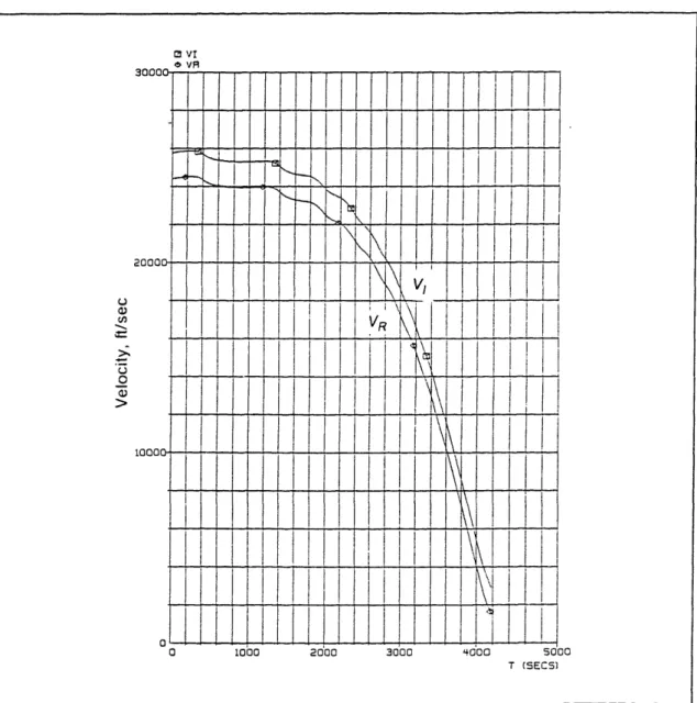
Closed-Loop Velocity History for the Maximum Downrange Case ...

Closed-Loop Heat Rate History for the Maximum Downrange Case ...

Closed-Loop Heat Load History for the Maximum Downrange Case ...

Closed-Loop Downrange History for the Maximum Downrange Case ...

Closed-Loop Crossrange History for the Maximum Downrange Case ...

Closed-Loop Altitude History for the Maximum Crossrange Case ...

Closed-Loop Velocity History for the Maximum Crossrange Case ...

Closed-Loop Heat Rate History for the Maximum Crossrange Case ...

Closed-Loop Heat Load History for the Maximum Crossrange Case ...

Closed-Loop Downrange History for the Maximum Crossrange Case ...

Closed-Loop Crossrange History for the Maximum Crossrange Case ...

Closed-Loop Altitude History for the Minimum Downrange Case ...

Closed-Loop Velocity History for the Minimum Downrange Case ...

Closed-Loop Heat Rate History for the Minimum Downrange Case ...

Closed-Loop Heat Load History for the Minimum Downrange Case ...

Closed-Loop Downrange History for the Minimum Downrange Case ...

Closed-Loop Crossrange History for the Minimum Downrange Case ...

44. Angle of Attack Comparison for the Maximum Downrange Case ...

45. Bank Angle Comparison for the Maximum Downrange Case ...

46. Angle of Attack Comparison for the Maximum Crossrange Case ...

47. Bank Angle Comparison for the Maximum Crossrange Case ...

48. Angle of Attack Comparison for the Minimum Downrange Case ...

100 101 102 103 104 105 106 107 108 109 110 111 112 113 114 115 116 117 118 119 120 121 122 123 124 125 27. 28. 29. 30. 31. 32. 33. 34. 35. 36. 37. 38. 39. 40. 41. 42. 43. . . . .. . . 99

49. Bank Angle Comparison for the Minimum Downrange Case ... ... 126

50. Bank Angle Versus Time Comparison for Heat Rate Control ... 127

51. Angle of Attack Versus Time Comparison for Heat Rate Control ... 128

52. Heat Rate Versus Time Comparison for Heat Rate Control ... 129

53. Bank Angle Versus Velocity Comparison for Heat Rate Control ... 130

54. Angle of Attack Versus Time Comparison with Overcontrol ... 131

LIST OF TABLES

Table Page

1. Characteristics of the ERV and Trajectory Entry Conditions ... 73

2. Dispersions Used in Performance Study ... 73

3. Dispersed Cases for Maximum Downrange Region ... .... 74

4. Dispersed Cases for Maximum Crossrange Region ... 75

5. Dispersed Cases for Minimum Downrange Region ... ... 76

6. Maximum Downrange Region Closed-Loop Results ... ... 77

7. Maximum Crossrange Region Closed-Loop Results ... 77

SYMBOLS

a = acceleration magnitude

a = acceleration vector

a, = inertial acceleration measured by the inertial measurement unit

A, = total inertial acceleration vector

AOTV = Aerobraking Orbital Transfer Vehicle

BTU = British Thermal IJnit

c = mean aerodynamic chord

cos(A¢) = cosine of incremental lift for heat rate control

C' = proportionality factor for the linear viscosity-temperature relationship

Co = aerodynamic drag coefficient

CL = aerodynamic lift coefficient

C, = speed of sound

CPU = central processing unit

CR = crossrange

CSDL = The Charles Stark Draper Laboratory, Inc.

det = determinant of sensitivity matrix

DR = downrange

DOF = degree of freedom

ERV = Entry Research Vehicle

fearth = flattening of oblate Earth

F, = inertial force vector

g = gravitational acceleration magnitude

= Global Positioning System

h = altitude

/h = derivative of altitude with time

h = second-derivative of altitude with time

h, - scale height for exponential atmosphere model

i = unit vector

= second zonal harmonic coefficient

JSC = Lyndon B. Johnson Space Center

k = term in geodetic to geocentric latitude conversion

K = term in heat rate control equation

K = velocity vector term in the integration algorithm

K' = acceleration vector term in the integration algorithm

KAt =- gain on acceleration magnitude in variable time step equation

KLID =multiplicative scale factor on the nominal L/D

K6 = gain on heat rate error in heat rate control equation

Kb = gain on rate of change of heat rate in heat rate control equation

KP = multiplicative scale factor on the standard density

K, = gain in first-order filter for density smoothing

K2 = gain in first-order filter for L/D smoothing

LID = lift-to-drag ratio

LaRC = Langley Research Center

m = mass

M =Mach Number

MrF = inertial-to-Earth-fixed transformation matrix

MO = mean molecular weight of air at sea level

n.m. = nautical mile

NASA = National Aeronautics and Space Administration

POST = Program to Optimize Simulated Trajectories = dynamic pressure

Q = heat load

Q = heat rate

Q = time rate of change of heat rate

R = position vector magnitude

Requator = radius of oblate Earth at equator

R, = inertial position vector

Rpole = radius of oblate Earth at pole

Re = Reynolds Number

S = Sutherland's constant in viscosity equation

S = aerodynamic reference area

SEADS = Shuttle Entry Air Data System

tG,rT = Greenwich mean time

T' = reference temperature

TM = molecular scale temperature

Tstatc = freestream static temperature

Twa.1 = wall temperature

TAEM = Terminal Area Energy Management

V = Viscous Interaction Parameter

V, = magnitude of inertial velocity

V, = inertial velocity vector

VR = magnitude of Earth-relative velocity

VR = Earth-relative velocity vector

z = geocentric colatitude of the postion vector

P/ = angle of sideslip

6 = small incremental change

A = incremental change

y = ratio of specific heats for air

= longitude

/. = coefficient of viscosity for air

/.z = Earth gravitational constant

4earth = Earth's rotation vector

c. -= natural frequency of heat rate control response

= bank angle

= universal gas constant

p = atmospheric density

= standard deviation

-r = time constant of filter

sx -= damping ratio of heat rate control response

SUBSCRIPTS aero = aerodynamic c = geocentric cmd = command d = desired des = desired

e = error

El = entry interface

f

=

final

g = geodetic

imu = inertial measurement unit

inplane = projection of target unit vector into plane formed by the

position vector and the relative velocity vector

lat = direction perpendicular to the plane formed by the position vector

and the relative velocity vector

lift = lift term

lim = limiting value or boundary

LID = lift-to-drag ratio

max = maximum

min = minimum

nom = nominal

perpen = direction perpendicular to the plane formed by the position vector

and the relative velocity vector

pole = direction of the north pole

R = direction of the position vector

si = sea level

std = standard value

t = target aim point

SUPERSCRIPTS

EF = coordinatized in Earth-fixed coordinates

imu = value measured by inertial measurement unit on current cycle

imu past = value measured by inertial measurement unit on past cycle

A = estimated or measured

1.0 INTRODUCTION

Routine access to space and the maintenance of a Space Station will increasingly require greater flexibility in mission planning and the requirement for lower system mainte-nance costs. The launch and recovery phases of space flight have historically been the most demanding phases of space flight and therefore require the most development effort and investment. Mission flexibility requires more frequent launch and deorbit opportunities. For the case of re-entry vehicles, deorbit opportunities are defined by the ranging capability of the vehicle. A high L/D vehicle increases the available deorbit opportunities increasing mission flexibility. High L/D vehicles also are of interest for over-flight missions for the pur-pose of reconnaissance.

Entry guidance algorithms developed to date have been highly vehicle-specific and required great development and maintenance efforts over the life of the vehicle. These algo-rithms were not applicable to other vehicles without extensive modification.

This study seeks to design an adaptive entry guidance algorithm that maximizes the usable footprint by making full use of the available vehicle capability. This algorithm should also be easy to maintain throughout the vehicle definition phase and operational life. Mini-mizing the number of mission-dependent input parameters (I-loads) is desirable. The algo-rithm should also be easily transported to other vehicles to minimize development cost. Transportability is accomplished by minimizing vehicle-specific features of the algorithm. Explicit heat rate control should be provided to allow full use of the entry corridor up to the heat rate limits.

This study seeks to design such an algorithm. A candidate entry guidance algorithm is defined for the NASA Entry Research Vehicle (ERV), but is easily adapted to other vehicles with minimal modification. The proposed algorithm attains almost complete coverage of the achievable footprint, while employing a simple one-phase entry algorithm with explicit heat

rate control. Vehicle-specific features and I-loads are minimized, reducing algorithm

devel-opment and maintenance costs.

The ERV [1] is a proposed high-performance entry vehicle designed as a test bed for future technology development in the areas of:

1. Maneuvering entry/synergetic plane change

2. Atmospheric uncertainties

3. Advanced thermal protection systems

4. Aerodynamic/aeroheating prediction

5. Adaptive guidance and navigation

6. Load-bearing thermostructures

The ERV is designed for deployment from the Space Shuttle, after which the ERV enters the atmosphere for demonstration of the synergetic plane change, over-flight, and entry mis-sions. Figure 1 on page 78 shows a three-view drawing of the ERV and the surface areas of the aerodynamic control surfaces. Also seen is the size of the ERV in relation to the diam-eter of the Shuttle payload bay in which the ERV must'fit.

2.0 MOTIVATION

2.1 INTRODUCTION

The goal of any entry guidance algorithm is to successfully guide the vehicle to the desired final state for the largest range of dispersions possible without violating any vehicle constraints while also maximizing the achievable footprint. It is also desirable to minimize the mission and vehicle-specific aspects of the guidance algorithm so as to minimize pre-mission analysis and planning. Transportability of the algorithm from one vehicle to another significantly reduces guidance algorithm development effort and cost.

To maximize the footprint attainable, the guidance algorithm must follow the optimal path to any particular point in the footprint. The algorithms developed to date for such vehi-cles as the Apollo capsule [2] and the Space Shuttle [3] have attempted to do this by fitting the optimal trajectory with phases that follow important parameters (reference profiles) over some range of conditions. These guidance algorithms were required to be computationally

efficient because of the limited on-board computer resources available. Analytic

expressions for the reference profiles allowed for low execution time and tailoring of the tra-jectory for vehicle-specific constraints. For example, trajectories for these vehicles had to be shaped to reduce and control the maximum heat rate experienced below that allowed for the available thermal protection system materials.

The Space Shuttle entry guidance system employs three major modes with seven phas-es: 1. Entry a. Pre-entry b. Temperature control c. Equilibrium glide d. Constant drag e. Transition

2. Terminal Area Energy Management

3. Approach and Landing

Except for the pre-entry phase which is open-loop, each phase is described by an analytic expression relating the desired drag and altitude rate (the measured feedback terms used) to the desired profile. Because the algorithms are tailored for a particular vehicle and the reference profiles do not follow the optimal profile to all points in the footprint, guidance algorithms developed to date can not be easily adapted to other vehicles or provide full cov-erage of the theoretically achievable footprint.

The next generation of entry vehicles will not be so constrained due to advances in ther-mal protection system materials and computer technology. For example, flight computers are now capable of supercomputer speeds on the order of 40 million instructions per second utilizing parallel processing architecture [4]. A different approach to guidance that attempts to follow an optimal profile to maximize footprint capability is therefore possible.

The proposed approach is a predictor-corrector algorithm that numerically predicts the final state for a particular control variable history and then corrects the control variable his-tory to satisfy the specified final state constraints. This approach, proposed previously for

various guidance problems, has most often been impractical because of the long trajectories that must be predicted and the slow computer speeds.

Such an approach has been employed for the Space Shuttle Powered Explicit Guidance (PEG) [5] used for second stage ascent and orbit insertion burns where the trajectory is short enough to be predicted with the available computer resources. The Shuttle algorithm numerically predicts the gravitational effects during the powered flight phase with a 10 step integration of the 500 second trajectory.

A predictor-corrector has also been proposed for Aerobraking Orbital Transfer Vehicles (AOTV) [6] which would utilize more advanced computers. This algorithm numerically inte-grates the equations of motion along a skimming trajectory through the upper atmosphere that is approximately 500 seconds long and requires about 100 integration steps.

The trajectories flown by the ERV or any high L/D entry vehicle are typically from 30 to

100 minutes long from entry interface (400K feet) to landing, so the computational demand for such an algorithm is very gruat early in the entry when the time to landing is long. How-ever, because the entry is long and the vehicle has excess ranging capability for all but a small region along the edge of the footprint, the accuracy of the early predictions need not be as high as for the later predictions. Hence, large time steps can be used early in the pre-dictor algorithm. Later, when the vehicle nears the landing site, the time remaining is short, and hence, the prediction is short. This allows the predictor-corrector to be executed more often near landing just like the current analytic algorithms. Throughout the entry, vehicles using an analytic guidance algorithm with reference profiles must closely follow the refer-ence profile if the assumed referrefer-ence profile is to guide the vehicle to the correct final state. A predictor-corrector effectively recomputes a new reference profile each time it is executed, so the guidance execution rate can be much lower than that for analytic algorithms.

2.2 DISPERSIONS

Before the guidance algorithm can be designed, the possible dispersions that may affect the trajectory must be considered. The Shuttle entry guidance system is required to reach the Terminal Area Energy Management (TAEM) interface with less than a 2.5 nautical mile position error from the target aim point. The dispersions of significance to an entry vehicle trajectory include: 1. Vehicle characteristics a. Mass b. Aerodynamics c. Maneuver rates 2. Environment characteristics a. Atmospheric density b. Atmospheric winds

c. Atmospheric properties influencing aerodynamic flow regimes (temperature,

mean free path, etc.)

3. Initial entry state vector

a. Velocity

b. Flight path angle

c. Heading

4. Propagation errors in navigation state vector

Of these potential dispersion sources, only the vehicle mass, aerodynamics, and the atmospheric density and winds will be significant. By the early 1990's, almost perfect navi-gation can be expected through use of the Global Positioning System (GPS). If the deorbit burn guidance and control systems are assumed to correctly guide to the navigated state

and there are no navigation errors, then the dispersions in the initial entry state vector are negligible.

The vehicle mass should be known accurately, so for this study, a 3 error of +5% is assumed. Experience from the Space Shuttle program shows that the vehicle aerodynamics should be known to within +5% for the force coefficients on the first flight. Only the stability

derivatives and control effectiveness were missed significantly [7]. Even though the force

coefficients may be known to excellent accuracy, reduced control effectiveness can reduce the possible trim angle of attack range reducing the maximum L/D achievable. Therefore,

for this study, a +10% dispersion in the lift and drag coefficients is considered. It should be

noted that the first few flights of a new vehicle are usually targeted to the middle of the foot-print to maximize margin and allow for accurate determination of the vehicle characteristics before the full ranging capability of the vehicle is used. After the first few flights, the aero-dynamic characteristics should be known to within a few percent, so only about a +3% dis-persion must be considered.

The atmospheric dispersions were obtained from two sources. Reference [8] specifies the atmospheric dispersions to which aerospace vehicles must be designed. The average of the steady state winds at four geographic locations is shown in Figure 2 on page 79. This model was incorporated into the simulator environment with a magnitude scale factor to simulate less than worst-case winds. The wind direction was selected for each run made

with winds and held constant throughout the trajectory. Reference [8] specifies Reference

[9] as the source for atmospheric density dispersions. However, the recent Shuttle flights

have provided estimated density data of a quality never before available. Atmospheric den-sity profiles derived from Shuttle accelerometer measurements of the normal force acceler-ation and the estimated normal force coefficient and relative velocity vector are presented in

derived density profiles for the first 12 Shuttle flights. Of particular interest is the range of

dispersions seen: -47% to +12%. Figures 4 on page 81 and 5 on page 82 show the density

profiles for the STS-1 and STS-9 Shuttle flights. High frequency density shear components and constant density biases from the standard atmosphere are seen. For this study, con-stant density biases of +30% and the Shuttle derived density profiles from Reference [10] were used.

2.3 REFERENCE TRAJECTORIES

The size of the footprint for a particular vehicle is determined by the range in vehicle

L/D and the constraints placed on the trajectory such as heat rate limits. The edges of the

footprint correspond to the use of maximum or minimum UD. Maximum downrange or

crossrange, for example, requires maximum L/D, while minimum downrange requires

mini-mum L/D.

The determination of the optimal angle of attack and bank angle control histories for

maximum crossrange and downrange has been the topic of many papers [11] [12] [13] .

Wagner [12] used several optimization techniques to evaluate the maximum crossrange achievable for a multiphase bank angle history flown at maximum ULD. The multiphase bank profiles considered are shown in Figure 6 on page 83. It is seen that as the number of phas-es increasphas-es, the multiphase profile approachphas-es the optimal continuous profile also shown in this figure. It was determined that a three-phase bank angle profile as illustrated in Figure 6

achieved almost the same crossrange as a continuous bank profile. This is shown in

increases, the optimum bank angle profile approaches a continuous profile that is almost lin-ear with velocity as shown in Figure 8 on page 85. It was also hown that flying at the maxi-mum L/D maximizes the crossrange attained.

This result is confirmed in Reference [13] which utilized a nonlinear programming tech-nique to optimize the Space Shuttle trajectory for the maximum downrange and maximum crossrange cases. The maximum downrange trajectory requires flying at zero bank angle and at the angle of attack corresponding to maximum L/D as shown in Figure 9 on page 86. The control histories for the maximum crossrange case are shown in Figures 10 on page 87 and 11 on page 88. Again, the optimal control history is the angle of attack corresponding to maximum L/D and an almost linear bank angle profile with velocity.

Optimized trajectories for the ERV were reported in Reference [14]. These trajectories were determined using the Program to Optimize Simulated Trajectories (POST) [15] and imposed the following constraints on the trajectories:

1. Maximum heat rate of 125 BTU/sq ft/sec

2. Maximum heat load of 150K BTU/sq ft

The achievable footprint with these constraints, reported in Reference [14], is shown here in Figure 12 on page 89 . Subsequently, the heat load limit was increased to 175K BTU/sq ft resulting in the larger footprint shown in Figure 12. As will be seen, these footprints omit a large area in the minimum downrange region that is achievable within the heating con-straints. Also shown is the footprint of the Space Shuttle which has a maximum hypersonic

UL/D of 1.2 as compared with 1.8 for the ERV.

Figure 13 on page 90 shows the altitude history for the maximum downrange, maximum crossrange, and minimum downrange cases. Figures 14 on page 91 and 15 on page 92

show the bank angle and angle of attack histories for these trajectories. Figures 16 on page 93 and 17 on page 94 show the heat rate and heat load histories for these cases.

Figure 15 shows that the constant angle of attack corresponding to maximum L/D is flown for the edge of the footprint except for the minimum downrange case. For the mini-mum downrange case, the angle of attack corresponding to the minimini-mum L/D on the back side of the L/D curve (high drag coefficient) is flown early, followed by a ramp in angle of attack starting at 1500 seconds after entry interface. This ramp corresponds to the vehicle actually turning around and flying slightly back uprange, so maximum L/D is desired later to maximize the distance flown uprange.. The angle of attack for the maximum downrange case is slightly greater than that for maximum L/D because this trajectory exceeds the heat load limit f flown at maximum L/D. The maximum downrange region of the footprint Is therefore limited by the heat load limit set for the ERV. If the limit were relaxed, flight at maximum L/D would allow a longer downrange trajectory.

Figure 14 shows that the bank angle profile for maximum crossrange is approximately linear with time which is almost linear with velocity, which suggests that a linear bank angle profile with velocity is sufficient. The maximum downrange case has a constant bank angle of zero which is again linear with velocity. The minimum downrange case does not have a linear bank profile. As was mentioned previously, for this case, the vehicle turns around and

flys back uprange.

The results of these studies suggest that use of a constant angle of attack profile and a linear bank with velocity profile will capture a large portion of the achievable footprint. As will be seen in the results, these profiles suffice to capture most of the footprint reported in

out-side the reported footprint. Only a small area of the reported footprint in the minimum downrange region is unachievable.

Also of interest are the peaks in heat rate seen in Figure 16. Because the peaks in heat rate are very short, explicit control of the heat rate should be possible in the maximum heat rate regions without significantly impacting the giidance.

2.4 GUIDANCE APPROACH

The guidance design will attempt to maximize the size of the footprint while flying a con-stant angle of attack profile and a linear bank angle with velocity profile. The predictor algo-rithm integrates the equations of motion forward in time using the assumed control profile and the necessary environment and vehicle models. The corrector then determines (using multiple predicted trajectories with various control histories) the sensitivities of the final

state constraints to the control variables. The sensitivities are then used to compute the

required control variable values to reach the desired final state conditions. Heat rate control is provided locally during the regions of maximum heating without significantly affecting the assumed control histories. Also, in-flight measurements are utilized to increase the accura-cy of the predicted trajectories by compensating for off-nominal conditions.

Such a simple profile for the maximum downrange and crossrange cases simplifies the modeling of the control histories in the predictor. The only remaining question is how much

Footprint" on page 57, such a profile achieves almost complete coverage of the achievable footprint.

Also of concern is the linearity and convergence properties of the final state constraints with the control variables. As will be seen, over almost all of the footprint except near the edges, the constraints are highly linear and convergent with the control variables. Opera-tionally, only about 75% of the achievable footprint is used to nsure guidance margin. Thus, the question of nonconvergence near the edges is avoided.

3.0 GUIDANCE DESIGN

3.1 INTRODUCTION

This section describes the mplementational details of the guidance scheme described In the previous section. The equations of motion and environment and vehicle

character-Istics modeled in the predictor algorithm are described. The corrector algorithm to control

the final state constraints with the two available control variables is derived. Also derived are the heat rate control and in-flight measurement algorithms. The heat rate control algo-rithm provides control of the peaks in stagnation heat rate during the early portion of entry. The in-flight measurement algorithm utilizes accelerations measured by the navigation sys-tem to more accurately model the expected environment and vehicle characteristics in the predictor algorithm. Because the predictor-corrector algorithm is computationally intensive, areas where significant execution time savings have been or can be realized are ndicated. Program listings of the algorithm coded in the HAL/S computer language are presented in

"Appendix B. ALGORITHM PROGRAM LISTINGS" on page 135.

As will be seen, the only inputs to the guidance system are the environment and vehicle models, the assumed control profiles, and the navigated state vector. The state vector is an input to any guidance system. The other inputs are developed for the analysis of any new

vehicle. Therefore, the guidance system is highly transportable between vehicles because

only the vehicle characteristics and aerodynamics model must be changed for a new vehi-cle.

3.2 UNIT TARGET VECTOR

The target aim point to which the vehicle is to be guided is specified by the longitude and geodetic latitude of the Terminal Area Energy Management (TAEM) interface point which occurs at 80K feet for the Shuttle. This point is selected based on the guidance algorithm employed during the TAEM guidance phase. TAEM guidance provides precise control of vehicle energy during the final stages of entry to guide to a specified runway with acceptable energy. For computational ease, the longitude and geodetic latitude are converted to a tar-get unit vector in Earth-fixed coordinates by first computing the geocentric latitude from,

=

tan

tang) )

(

(1)

where,

k R= =Rator 2 (2)

The unit target vector is then computed from,

cos(q5) cos(i.)

jEl = /cos(o)

sin(A)

(3)

L

(4) where, where, i, = sin(tb,) i, = cos(A) /1 - i i, = sign(A) /1-ix-i2

3.3 COMMANDED ATTITUDE COMPUTATION

(5)

(6)

(7)

Because the predictor can not be executed as frequently as analytic guidance algo-rithms early in the entry, and because it in fact does not have to be executed as frequently, it is necessary to update the commands sent to the vehicle autopilot more frequently than the predictor-corrector execution rate. Typically, this would be done at the rate of current analytic guidance algorithms, e.g., the Space Shuttle rate of .52 hz. The commanded bank

angle, ,,, is computed for the linear bank with velocity profile as shown in Figure 18 on

page 95 from the desired bank angle, Ad, and the current navigated inertial velocity

magni-tude, V,,

(8)

V, - V,

to yield the near-optimal linear bank with velocity profile. The desired angle of attack con-trol history is a constant angle of attack, and therefore,

acmd = ad (9)

As implemented in the current design, the guidance algorithm executive is executed at 1.0 hz. The attitude commands are updated at this frequency using Eq. (8) and (9) . The pred-ictor-corrector algorithm is executed at .02 hz. during the entire entry phase, although it is

practical to run it much more frequently late in the trajectory when the length of the

trajecto-ry to be predicted is short. The possible execution rate of the predictor-corrector for a typi-cal flight computer is addressed in Subsection "4.8 Algorithm Execution Time" on page 66.

3.4 CORRECTOR ALGORITHM

The corrector algorithm is executed to update the commanded attitude control history to be flown. The guidance algorithm controls to two final state constraints, downrange error and crossrange error, using two control variables, a constant angle of attack and the inter-cept of the bank profile at the entry interface velocity as shown in Figure 18 on page 95 and

expressed in Eq. (8) .

Expanding the downrange and crossrange errors in a Taylor series expansion of the control variables and neglecting the second-order and higher terms yields,

OR ,

aDR,

ADR, = Ad + DR +... (10)

A CRe

aCR

+

a

_d

+

and +

(11)

To intercept the target, the change in the constraint errors must null the predicted errors, or,

ADRe A CR, = -DR, -CR, (12) (13)

Equations (10) through (13) provide a set of two simultaneous equations in two unknowns,

aDR, ODR, e

a1d ° 4radl

aCR, aCR LA dj

aad a d

which are solved for the control variable changes required,

DR, = ( 0 _CR,

-od

CR)I

de

Od

where det is the determinant of the matrix in Eq. (14).

(15)

(16)

The partial derivatives are approxi-mated by finite difference equations of the form,

DRe(0d = 3) -

DR,(bd

= ,)

There are four partial derivatives that must be evaluated. They can be evaluated from three predicted trajectories with control histories selected as:

[-DRe L-CReJ (14) Aad

Ad

1.

a,

(d

2.

3.

where the primes denote the control variables from the previous guidance solution. The new guidance commands are then,

ad =

a'd

=d = O'd + Ad

(19)

Protection must be provided for the.case where the determinant in Eq. (15) and (16) is small or identically zero which corresponds to a loss of control authority of the control vari-ables over the control constraints. In this case, no change is made to the control varivari-ables, and the guidance command from the previous cycle is used. As the vehicle approaches the TAEM interface altitude, the control authority decreases. Large control variable changes

become necessary to null the constraint errors in the short flight time remaining. This

prob-lem can be avoided in one of two ways. First, the guidance commands can be frozen at a selected point before the termination altitude. For entry guidance, this approach is not pre-ferred because the vehicle still has not landed. Alternatively, the target aim point can be lowered below the TAEM interface altitude point at which TAEM guidance is activated. The decreasing control authority problem is therefore reduced.

For the simulated trajectories in this report, the first approach is employed because it is desired to evaluate guidance performance by considering the dispersions in the final state at the TAEM interface altitude. Because the guidance algorithm controls only the final state and not the intermediate states, it is necessary to target for the point at which the guidance is terminated.

3.5 PREDICTOR ALGORITHM

3.5.1 Introduction

The predictor algorithm is a simplified three-degree-of-freedom (3-DOF) trajectory simu-lator complete with models for those environment and vehicle characteristics necessary to model the translational equations of motion of the vehicle. Because the predictor is compu-tationally intensive, the algorithm must be carefully designed to minimize computation, and the coding of the algorithm in a particular computer language should make use of any lan-guage-specific features to reduce computational requirements. Also, because the corrector only utilizes the final state vector errors to correct the control variables, only the accuracy of the predicted final state vector need be considered in selecting those effects to be modeled.

The environmental effects of concern for the long trajectories flown by entry vehicles

over large altitude and velocity ranges are:

1. Variation of atmospheric properties with altitude

2. Earth oblateness effect on gravity vector

3. Effect of atmospheric rotation with Earth on relative velocity vector

4. Movement of runway due to Earth rotation

The vehicle characteristics of importance are:

1. Vehicle mass

2. Aerodynamic coefficient variation with flight regime

3. Aerodynamic coefficient variation with angle of attack

4. Control history during trajectory

1. Vehicle mass variation from nominal

2. Winds

3. Atmospheric density variation from nominal atmosphere

4. Aerodynamic coefficient variation from nominal

These dispersions can be measured in-flight because they affect the sensed acceleration measured by the vehicle's inertial navigation system. The estimation of these dispersions is discussed in Subsection "3.6 Estimators" on page 48.

The predictor performs the following computations upon being called by the corrector with a desired control variable history:

1. Initialize the predictor state to the navigated state vector

2. Compute any ancillary parameters from the state vector

3. Compute the total acceleration vector from the predictor state vector and the

envi-ronment and vehicle models using the control variable profiles specified by the cor-rector

4. Integrate the equations of motion forward in time one time step

5. Check the predictor termination conditions

a. Repeat steps 3 and 4 if the conditions are not met

b. Continue on to step 6 if the conditions are met

6. Compute and return to the corrector the final predicted state errors from the target

state vector and the predicted final state vector

3.5.2 Equations of Motion

The corrector provides a time-homogeneous navigated state vector comprised of,

1. The GMT time tag of the state vector, tGwr

2. The inertial position vector, R,

Also provided is the control variable history to be followed for the prediction. The equations of motion to be integrated are,

d R,

dt

dV,

= A,

dt

The acceleration is computed from the atmosphere and vehicle models as follows,

F, -~

-A, - m = g, + aaeo

The gravitational acceleration, g,, is computed including the J2term as,

(21) (22) 9g IR, 12 JR, 2 where, 3 Rquat, Ig = 'R + - J2 ((15 2) iR

+

The aerodynamic acceleration, a,,o, is computed from,

aaero =- alf ift + adr,ag drag

where, CL, q S a,,,t m (23) (24) (25) (26) (27)

adag = m (28) -- P Vz (29) q = ₌ vVRV _{VR * VR(30)} (30) VR = Vl - ,,eanrXR. (31) idrag = (32) I v

ilift = (idra X i,) cos(k) + ia

sin(X)

(33)

I_R X drag

h,, = (34)

I

jR = (35)

IR, I

The acceleration due to lift, a,,ft, is more easily computed from,

a,,f = L a, (36)

since the nominal lift-to-drag ratio, L/D, is corrected using in-flight accelerometer

measure-ments of the actual vehicle sensed aerodynamic accelerations.

The atmospheric density, p, is computed by the atmosphere model using the position vector, R.. The 1962 U.S. Standard Atmosphere model is employed and is described in Ref-erence [16]. If another atmosphere model is selected as being a more accurate estimate of the day-of-flight atmosphere, this model would replace the 1962 U.S. Standard Atmosphere

sources as the GRAM Atmosphere [9] or even day-of-flight measurements to more accu-rately model the expected atmosphere in the predictions. The level of accuracy required in the atmosphere model will depend on the vehicle ranging capability and the amount of that capability to be.used for a particular entry. Entries to the edges of the footprint will demand

a very accurate atmosphere model.

The aerodynamic coefficients are highly vehicle dependent. To minimize computational requirements, they should be updated during the prediction as infrequently as possible. Of course, the update frequency required depends on the trajectory flown and the rate of change of the aerodynamic coefficients with flight regime change. The aerodynamic

coeffi-cient model for the ERV is presented in "Appendix A. ERV AERODYNAMICS MODEL" on page 133.

The density, p, from the atmosphere model and the lift-to-drag ratio, L/D, from the aero-dynamic model are both corrected by in-flight measurements as covered in Subsection "3.6 Estimators" on page 48. The estimated dispersions are compensated for using the following equations,

p = Kp Ptd (37)

KL CL) (38)

D 6 Co

where the density and lift-to-drag ratio scale factors, Kp and KL, are provided by the

estima-tor and are held constant throughout the prediction being made.

The control history to be followed is the constant angle of attack, ad, and the linear bank

VI-VI

~b -~d

(39)

VE,- V,

where d is the intercept of the linear bank angle profile at the entry interface velocity, VE,.

Because the entry interface and final velocities are not known a priori, and because small variations in them have little effect on the predicted trajectory compared with the selected control variables' values, the velocities are selected as constant values that cover all expected dispersions in the entry and final velocities. These values are,

VE, - 26,000 ft/sec

Vf = 1,000 ft/sec

3.5.3 Integration of the Equations of Motion

The equations of motion are integrated using the 4th order Runge-Kutta algorithm with a variable time step to minimize the number of time steps required to integrate the trajectory to the final state. The 4th order Runge-Kutta algorithm requires four evaluations of the acceleration per time step, but permits a time step more than four times as large as an algo-rithm requiring only one acceleration evaluation per time step. The Runge-Kutta solution [17] for the differential equations of motion of the form,

dRI

d t V, (40)

dt

dV f(t, R V) (41)

-'(+

-')+

4

t

--R,(t + At) = --R,(t)+

-

6 (Ko 2K + 2 K + K,)2

+ )

_2'

+ At 2'

~

~

The time step is varied inversely with the total acceleration on the vehicle. This method of time step control was selected because of its simplicity. The time step control equation is of the form, KA, At = _ (52) IA, I (43) (44) (45) (46) (47) (48) (49) (50) (42)

and the time step is limited between a minimum and maximum value,

At = midval(Atm,,, At, tma),, (53)

The optimization of the integration algorithm is important in developing a flight quality algorithm, but is beyond the scope of this study. Higher-order integration algorithms with

time step control methods [17] may yield significant reductions in the required computation

time.

3.5.4 Termination Conditions for the Predictor

After each integration time step, the predicted state is compared with the termination condition. The termination condition is defined by the altitude of TAEM interface (80K feet). Because the predicted state at the TAEM interface altitude may have a relatively large alti-tude rate and range rate, the predictor must be terminated accurately to provide an altialti-tude- altitude-homogeneous set of predicted state errors. Also, the variable time step control may allow large integration time steps if the acceleration is low near the final state, further complicat-ing the task of terminatcomplicat-ing accurately. Reasonable altitude homogeneity is ensured by forc-ing use of the minimum integration time step startforc-ing some safe altitude above the termination altitude.

3.5.5 Final State Error Computation

The final state errors are computed from the unit target vector and the predicted final state vector. Because the target is fixed to the Earth and moves a significant distance

dur-ing the long entry trajectory, the rotation of the Earth must be considered. This is done by transforming the final state vector from inertial to Earth-fixed coordinates with the rotation matrix MEf which is computed from the predicted termination time, the known orientation of the Earth at some epoch time, and the known rotation rate of the Earth. This computation is performed in the Earth-Fixed-From-Reference subroutine of the predictor-corrector which may actually be a GN&C utility function also employed by the navigation principal function.

The downrange and crossrange errors are defined as shown in Figure 19 on page 96. The errors are computed by first computing the downrange (in-plane) and crossrange (per-pendicular) directions as follows,

RIF = MF R (54) REF I= E(55) 5 REF J VR = M V (56) EF VEF /een - (57)

I. x V

l

The downrange and crossrange errors are then,

DRe = Requator COs 1(i X iE,ane) sign((iRF x ipa,,ne) i/pen) · (59)

These errors have the dimensions of R,,,,tor and are converted to nautical miles for ease of interpretation.

3.5.6 Algorithm Coding

A few comments regarding implementation of the predictor are appropriate. The com-putations required to update the aerodynamic coefficients are the major computational load for the predictor. It was found that it is not necessary to update the aerodynamics on each of the four acceleration evaluations of the 4th order Runge-Kutta algorithm. They are there-fore only evaluated once each integration time step. The computational load could be reduced further if they are only updated when the independent variables (altitude, viscous interaction parameter, and Mach Number) change by a significant amount from the previous update. Also, although not done in this implementation, the aerodynamic coefficients should be curve-fit if possible to avoid a table lookup and interpolation implementation. It is noted

in Figures 20 on page 97 and 21 on page- 98 that the aerodynamic coefficients do not change

very much below 300K feet until the Mach Number decreases below 2, so perhaps, two tables or curve-fits would suffice instead of the thirty tables currently used.

3.6 ESTIMATORS

The final state predicted by the predictor algorithm for a particular control history is a function of the assumed environment and vehicle characteristics. The accuracy of the pre-dicted final state can be increased, and hence, the guidance margin increased, if in-flight

measurements are utilized to make the assumed models more accurately reflect the condi-tions actually experienced by the vehicle.

The accelerations modeled in the predictor are due to gravity and the aerodynamic forc-es. The gravity acceleration can be modeled to sufficient accuracy using standard gravity models. However, the aerodynamic accelerations are subject to significant variations due to uncertainties in the atmospheric density, atmospheric winds, vehicle aerodynamics, and vehicle mass. These uncertainties can be compensated for in the predictor by applying a multiplicative scale factor to the lift and drag accelerations modeled in the predictor that is equal to the ratio of the actual accelerations experienced to the predicted accelerations at any point in the trajectory.

The measured lift and drag accelerations are derived from the inertial measurement system sensed acceleration assuming a zero sideslip angle as follows,

A ^ - VR

adrag = -a, (61)

IVRI

a,, =

a,

where the inertial acceleration, a,, is computed by back-differencing the accumulated sensed velocity counts from the inertial measurement unit,

V;mu - V;mu paW

a, = (63)

In the predictor, the aerodynamic accelerations are,

C S 1 2

a,,t

D

Data from the Shuttle program [10] shows that the primary dispersion affecting the aerodynamic acceleration is in the atmospheric density. Further, over large altitude ranges, this dispersion can be modeled to an accuracy sufficient for the prediction process as a con-stant multiplicative bias. Therefore, for implementational purposes, the dispersion in the aerodynamic accelerations due to the atmospheric uncertainties will be lumped into a densi-ty scale factor as follows,

P K = (66) P Pstd where, A A 2 adrg m (67)

p

=

k~2a/

,,o,

,

and the values for the nominal vehicle characteristics and the nominal atmospheric density are determined using the predictor models for the vehicle state at the time of the measure-ment. Because the nominal ballistic coefficient is assumed in deriving the measured densi-ty, and the measured acceleration is due to the actual ballistic coefficient, uncertainties in the ballistic coefficient will be reflected in the measured density. The equation for the drag acceleration in the predictor is then,

adg = (co ) 2 VRKp Pptd (68)

or substituting for Kp from Eq. (66) yields,

ad.. (cmS) 1 V2 A (69)

A

ado = ad..g (70)

so the modeled drag is corrected for the dispersed drag coefficient, density, relative velocity,

and vehicle mass.

In general, the measured drag acceleration is a noisy signal and will exhibit short term

variations due to short lived local atmospheric dispersions [10]. Filtering of the density

scale factor is therefore necessary and is implemented using a first-order filter,

A

Kp = (1-K) Kp + K, P

P P std (71)

which has a time constant , r,, of,

=At

(

P In(1 -K)

where At is the sample rate of the measured drag acceleration, and K, is the filter gain. similar lift-to-drag ratio scale factor is derived and applied to the lift acceleration,

a,,ft

and,

A _A

a,

adrag

Again, filtering is necessary,

A

KL = (1-K 2) KL + K2

D ( ( )D nom

yielding a time constant, L, of,

At

ZL

A time constant of 25 seconds was selected for both the density and UD filters. This value filtered out the high frequency density shear components seen in the Shuttle profiles while still providing adequate response to long term disturbances.

3.7 HEAT RATE CONTROL

The primary trajectory constraint on entry vehicles is the maximum heat rate the vehicle can withstand. In general, the thermal protection system material is selected to withstand

the maximum local heat rate on any particular portion of the vehicle, and the material

thick-ness is selected to withstand the total integrated heat load ocer the trajectory. Accurate

pre-flight predictions of the expected heat rate during entry can significantly reduce the ther-mal protection system weight yielding significant performance increases for an entire mis-sion.

Inspecting the reference trajectories in Figure 16 on page 93 shows that sharp peaks in the heat rate occur. If these peaks are accurately controlled, and this control can be accom-plished using only short term departures from the predictor assumed control history, no sig-nificant departure will occur from the desired trajectory.

Heat rate control can be accomplished using either angle of attack, bank angle, or a combination of both. Of these, bank angle alone is preferred because a constant angle of attack trajectory is assumed and because angle of attack changes the vehicle drag coeffi-cient resulting in a rapid change in energy rate and a rapid departure from the desired tra-jectory. Also, most entry vehicles restrict the angle of attack range during maximum heat rate regions to reduce the area on the vehicle that must be protected from the high heat rate. Although the ERV does not need to restrict the angle of attack range, and hence, the guidance does not provide for such a capabilty, the restriction can be handled by replacing the constant angle of attack control history by a reference angle of attack control history

about which a constant angle of attack bias is applied for control.

Heat rate control is accomplished by computing the incremental bank angle required to

fly along the specified heat rate boundary (assumed to be a constant heat rate for any flight

regime) and then modulating bank angle according to the guidance value or the guidance value plus the incremental lift for heat rate control, whichever requires more lift up. Hence, no effort is made to pull the vehicle down into the atmosphere to follow the heat rate

bound--ary; instead, lift up is applied if the vehicle is flying "too low". The incremental lift for heat rate control is computed to provide a second-order control response as follows,

Kb . K .

cos(AO) = (- d

(-

(78)

q q

To fly along a constant heat rate boundary,

Qi, = constant (79)

and the desired rate of change of heat rate, Qd.., is,

(de = 0 (80)

so,

K,5 + K6

cos(AO) =

_

Q

+

Q

-

C,,(81)

q q

The stagnation heat rate is determined using the Engineering Correlation Formula [18] for a one foot radius reference sphere as,

(Q

: 17700 -'p (0 0) (82)

The time rate of change of heat rate, Q, is determined by back-differencing the heat rate

between guidance cycles,

I =Q Qpast. (83)

At

The equations of moion assuming small flight path angle yield,

Considering only the perturbations due to the incremental lift, cos(AO), from Eq. (81) yields,

m K-. + K ( - Qi,.) = 0 (85)

Proper selection of the gains K and K is accomplished by linearizing Eq. (85) in altitude

and assuming that the time rate of change of VR is small compared to the change in -.

With these assumptions,

=

d

_dh

ph

d'I

dh

dh

dt

Therefore, the homogeneous second-order differential equation in altitude is,

h + K K h + K K h = 0

where,

m 17700 10000 dh

The natural frequency and damping ratio of the second-order differential equation are,

wn = A/K K6 K K -2 co, (87) (88) (89) (90) (91) (86)

or alternatively, for a desired natural frequency and damping ratio, K6 and Kb are selected