THÈSE
En vue de l’obtention du
DOCTORAT DE L’UNIVERSITÉ DE TOULOUSE
Délivré par l'Université Toulouse 3 - Paul Sabatier
Présentée et soutenue par
SOFIA DARMARAKI
Le 17 avril 2019
Canicules océaniques en Méditerranée : détection, variabilité
passée et évolution future
Ecole doctorale : SDU2E - Sciences de l'Univers, de l'Environnement et de
l'Espace
Spécialité : Océan, Atmosphère, Climat Unité de recherche :
CNRM - Centre National de Recherches Météorologiques
Thèse dirigée par
MICHEL DEQUE et Samuel SOMOT
Jury
M. Michel CRéPON, Rapporteur M. Gabriel JORDA, Rapporteur Mme Claude ESTOURNEL, Examinatrice
M. Laurent LI, Examinateur M. Eric OLIVER, Examinateur M. Michel DEQUE, Directeur de thèse M. Samuel SOMOT, Co-directeur de thèse
adventure. For all these stimulating discussions that sparked new ideas while advancing the limits of the already existing ones. For all the moments that answers to the questions became even more interesting questions themselves. For all those afternoon meetings that I enjoyed acquiring new knowledge and alongside confidence through his always-encouraging words. But most important of all, for all the skills and tools that he taught me in order to follow the path of my dreams. I am also thankful to Florence, Pierre and Robin for their essential and timely contributions and help at any given moment I needed, and to the people of Meteo France in the technical (or not) part that were always willing to help me solving any kind of problem, that very often tended to appear.
Last but not least, I would like to express my gratitude to the wonderful friends from all over the world that I met during these amazing three years. For their sweet and uplifting support and friendship that was always a safe refuge to come back to in moments of difficulty. And of course, to my parents and all my family that, though far away, they have been always the strongest pylon, to which I always have and I always will lean on, no matter the corner of the planet I will set to explore.
Abstract . . . iv
R´esum´e . . . v
Introduction Fran¸cais . . . vi
List of Tables . . . xii
List of Figures. . . xv
1 Introduction 1 1.1 The Mediterranean Region . . . 2
1.2 Modeling of the Mediterranean Climate System . . . 6
1.3 Climate Change Scenarios and Uncertainty . . . 7
1.4 Projections for the Mediterranean Region. . . 9
1.4.1 Mean Climate . . . 9
1.4.2 Future evolution of Mediterranean Sea Characteristics. . . 10
1.4.3 Impacts on Marine Ecosystems . . . 17
1.4.4 Uncertainties in Mediterranean Future Projections . . . 19
1.4.5 Climate Extremes in the Mediterrranean . . . 22
1.5 Marine Heatwaves. . . 23
1.5.1 Driving Mechanisms . . . 24
1.5.2 Detection Methods . . . 30
1.5.3 Trends in the Past and the Future. . . 32
1.5.4 Impacts on Marine Ecosystems . . . 36
1.5.5 Subsurface Marine Heatwaves . . . 37
1.5.6 Marine Heatwaves in the Mediterranean Sea . . . 38
1.6 Conclusions . . . 42
1.6.1 Motivation of the study . . . 42
1.6.2 Scientific questions of the thesis . . . 43
2 Marine Heatwaves: Algorithm Description and Implementation 45 2.1 Model and Simulation . . . 46
2.2 Choosing the RCSM model. . . 48
2.3 Model Evaluation . . . 50
2.4 Observational Datasets . . . 53
2.5 Definition of Summer Mediterranean MHWs . . . 54
2.5.1 Objectives . . . 54
2.5.2 Designing the Algorithm . . . 54
2.5.3 Gap Days . . . 55
2.5.4 Example of a local MHW detection . . . 57
2.5.5 Spatial aggregation . . . 59
2.9 Conclusions . . . 71
3 Past summer Marine Heatwave Variability in the Mediterranean Sea 73 3.1 Introduction . . . 74
3.2 Materials and Methods . . . 76
3.2.1 Model and Simulation . . . 76
3.2.2 Observations . . . 76
3.2.3 MHW detection method . . . 76
3.3 Results . . . 77
3.3.1 Extreme Temperature Evolution. . . 77
3.3.2 Surface MHW characteristics . . . 77 3.3.3 Subsurface MHW characteristics. . . 79 3.3.4 MHW Seasonality . . . 80 3.3.5 MHW Spatial Distribution . . . 82 3.4 Discussion . . . 82 3.5 Conclusions . . . 85 3.6 Supplementary Material . . . 86
4 Marine Heatwave 2003: Driving Mechanisms 92 4.1 Methodology . . . 93
4.1.1 Temporal and Spatial Aggregation . . . 95
4.2 Analysis of MHW 2003 at basin-scale . . . 96
4.2.1 Ocean Heat Budget . . . 96
4.2.2 Atmosphere Heat budget . . . 99
4.2.3 Overall Attribution . . . 100
4.3 Regional MHW 2003 Analysis . . . 100
4.3.1 Western Mediterranean Basins. . . 102
4.3.2 Eastern Mediterranean Basins . . . 108
4.4 Conclusions . . . 113
5 Future Marine Heatwave Evolution in the Mediterranean Sea 114 5.1 Introduction . . . 115
5.2 Material and methods . . . 118
5.2.1 Model Data and Simulations . . . 118
5.2.2 Reference Dataset . . . 120
5.2.3 Defining Marine Heatwaves . . . 121
5.3 Results . . . 123
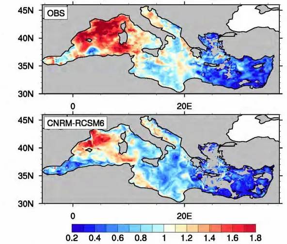
5.3.1 Model Evaluation . . . 123
5.3.2 Future Mediterranean SST evolution . . . 128
5.3.3 Future evolution of Mediterranean MHWs . . . 131
5.4 Discussion . . . 136
5.4.1 MHW detection method . . . 136
5.4.2 Model-Observation Discrepancies . . . 136
5.4.3 Model uncertainty . . . 136
5.4.4 MHW evolution and changes in SST . . . 137
5.5 Conclusions . . . 139
6.2 Conclusions et Perspectives (Fran¸cais) . . . 153
Annex 164
Evolution
The Mediterranean Sea is considered a “Hot Spot” region for future climate change and depending on the greenhouse emission scenario, the annual mean basin sea surface temperature (SST) is expected to increase from +1.5 °C to +3 °C at the end of the 21st century relative to present-day. This significant SST rise is likely to intensify episodes of extreme warm ocean temperatures in the basin, named as Marine heatwaves (MHWs), that are known to exert substantial pressure on marine ecosystems and related fisheries around the world.
In this context, the main aim of this PhD work is to study the past variability and future evolution of MHWs in the Mediterranean Sea. We propose a detection method for long-lasting and large-scale summer MHWs, using a local, climatological 99th percentile threshold, based on present-climate daily SST. MHW probability of occurrence and characteristics in terms of spatial variability and temporal evolution are then investigated, using additional integrated indicators (e.g. duration, intensity, spatial extension, severity) to describe past and future events. Within the PhD and depending on the applications, the detection method is applied to various datasets: In-situ observation at buoys, resolution satellite product, various high-resolution and fully-coupled Regional Climate System Models including the recently developed CNRM-RCSM6 and the multi-model (5), multi-scenario (3) Med-CORDEX ensemble. The detection method is first tested on the 2003 MHW in order to assess its sensitivity to various tuning parameters. We conclude that its characterization is partly sensitive to the algorithm setting. Hindcast and historical mode simulations show that models are able to capture well observed MHW characteristics.
We then assess past surface MHW variability (1982-2017) and their underlying driving mechanisms using the CNRM-RCSM6 model. We examine their characteristics from surface to 55m depth, where most thermal stress-related mass mortalities of Mediterranean ecosystems have been observed in the past. The analysis indicates an increase in duration and intensity of surface events with time, while MHWs of 2003, 2012 and 2015 are identified as the most severe events of the period. In particular, an anomalous increase in shortwave radiation and a lower-than-normal vertical diffusion and latent heat loss appeared to be responsible for the development of the MHW 2003, with wind playing a key role in the intensity of temperature anomalies at the sea surface. Differences on the dominant forcing, however, are sometimes evident in the different subbasin.
We finally use the Med-CORDEX RCSM ensemble to assess the future MHW evolution in the basin over 1976-2100. Our results suggest longer and more severe events with higher global-warming rates. By 2100 and under RCP8.5, simulations project at least one long-lasting MHW every year, up to 3 months longer, about 4 times more intense and 42 times more severe than present-day events. Their occurrence is expected between June-October affecting at peak the entire basin. Their evolution is found to mainly occur due to an increase in the mean SST but an increase in daily SST variability plays also a noticeable role. Up to mid-21st century MHW characteristics rise independently of the choice of the emission scenario, whose influence becomes more evident by the end of the period. Further analysis finally reveals different climate change responses in certain configurations, more likely linked to their driving global climate model rather than to the individual regional model biases.
This study provides a better understanding of Mediterranean Sea sensitivity to climate change considering for the first time the uncertainties related to global and regional climate models. We believe that this constitutes key information for the marine ecosystems and marine-related activities and societies in the basin that are under considerable risks due to the devastating effects of these events.
lution future
L’objectif principal de ce travail de th`ese est d’´etudier la variabilit´e pass´ee et l’´evolution future des ´episodes de temp´eratures oc´eaniques anormalement chaudes en M´editerran´ee. Ces ´
ev`enements, appel´es canicules oc´eaniques ou Marine Heatwaves en anglais (MHW), sont con-nues pour exercer une pression consid´erable sur les ´ecosyst`emes marins et les pˆecheries associ´ees un peu partout dans le monde.
Nous proposons une nouvelle m´ethode de d´etection automatique des MHWs d’´et´e bas´ee sur le 99`eme centile de la temp´erature quotidienne de la surface de la mer (TSM) en climat pr´esent et tenant compte de la diversit´e g´eographique de la zone. La probabilit´e d’occurrence des MHWs et leurs caract´eristiques spatio-temporelles sont ensuite ´etudi´ees. D’autres indicateurs int´egr´es tels que la dur´ee, l’intensit´e, l’extension spatiale maximale ou la s´ev´erit´e permettent de compl´eter la description des MHWs. Au cours de cette th`ese et en fonction des applications, la m´ethode de d´etection est appliqu´ee `a diff´erents types de donn´ees: observations in-situ aux bou´ees, produit satellitaire et diff´erents mod`eles haute r´esolution et coupl´es haute fr´equence du syst`eme climatique r´egional (RCSMs pour Regional Climate System Model en anglais) y compris le nouveau mod`ele CNRM-RCSM6 et l’ensemble Med-CORDEX multi-mod`ele (5) et multi-sc´enarios (3). L’algorithme de d´etection est d’abord test´e sur la MHW de 2003 afin de montrer qu’il est peu sensible aux diff´erents param`etres de r´eglage.
L’´evaluation des simulations r´etrospectives et historiques montrent que les RCSMs sont capables dans l’ensemble de bien reproduire l’occurrence et les caract´eristiques des MHWs observ´ees par satellite. Nous ´etudions ensuite la variabilit´e pass´ee des MHWs de surface (1982-2017) ainsi que leurs facteurs explicatifs en utilisant le mod`ele CNRM-RCSM6. Nous exam-inons, leurs caract´eristiques entre 20-55 m de profondeur, l`a o`u la plupart des mortalit´es de masse li´ees au stress thermique des ´ecosyst`emes m´editerran´eens ont ´et´e observ´ees dans le pass´e. L’analyse indique une augmentation de la dur´ee et de l’intensit´e des ´ev`enements de surface au fil du temps, tandis que les MHWs de 2003, 2012 et 2015 sont d´etect´ees comme les ´ev`enements les plus s´ev`eres de la p´eriode. Par ailleurs, pour la canicule 2003 des diff´erences importantes dans la contribution des ´echanges air-mer et de la diffusion vertical de chaleur sont mis en ´
evidence pour les diff´erents sous-bassins m´editerran´eens. Nous montrons ´egalement que la ten-sion de vent joue un rˆole cl´e sur l’intensit´e des anomalies de temp´erature en surface ainsi que leur propagation verticale.
Enfin, nous utilisons l’ensemble Med-CORDEX de RCSMs pour ´evaluer l’´evolution future des MHWs dans la r´egion sur la p´eriode 1976-2100. Nos r´esultats sugg`erent des ´ev`enements plus longs et plus s´ev`eres au fur et `a mesure que le r´echauffement climatique s’intensifie. D’ici `a 2100 et dans le cadre du sc´enario le plus pessimiste (RCP8.5), les simulations projettent au moins une MHW de longue dur´ee chaque ann´ee, jusqu’`a 3 mois plus longue, environ 4 fois plus intense et 40 fois plus s´ev`ere que les ´ev`enements actuels. On s’attend `a ce qu’elles se produisent entre juin et octobre, affectant au plus fort de leur extension l’ensemble du bassin. Cette ´evolution s’explique principalement par une augmentation de la TSM moyenne, mais l’augmentation de la variabilit´e quotidienne de la TSM joue ´egalement un rˆole notable. Jusqu’au milieu du 21`eme si`ecle, les caract´eristiques des MHWs augmentent ind´ependamment du choix du sc´enario d’´emission, dont l’influence devient plus ´evidente `a la fin de la p´eriode. Enfin, l’analyse individuelle des mod`eles r´ev`ele diff´erentes familles de r´eponses au changement climatique. Ces diff´erences s’expliquent plus probablement par le choix du mod`ele global for¸cant, plutˆot que par les biais individuels des mod`eles r´egionaux.
Introduction (Fran¸
cais)
La r´
egion M´
editerran´
eenne
La zone m´editerran´eenne est un bassin de transition semi-ferm´e bord´e par une zone temp´er´ee au nord et une zone subtropicale au sud et `a l’est. Par cons´equent, les variabilit´es des lati-tudes moyennes et tropicales influencent conjointement cette zone `a la topographie complexe compos´ee de montagnes abruptes, de cˆotes ´etroites, de glaciers permanents au nord et de zones d´esertiques au sud, cr´eant ainsi une r´egion tr`es sensible au changement climatique. De forts contrastes de temp´eratures et de pr´ecipitations sont observ´es au sein mˆeme du bassin qui re-groupe des climats temp´er´es, arides et montagneux. La r´egion se caract´erise par des hivers doux et humides et des saisons estivales g´en´eralement chaudes ou s`eches.
Gibraltar Ionian Levantine Black Sea Suez Canal Red Sea (Scirocco) (Mistral) (Bora) (Etesians)
Figure 1: R´egion m´editerran´eenne et ses sous-bassins. Circulation des eaux de surface est ´egalement illustr´ee (redessin´ee d’apr`es De Madron et al. (2011)). Les vents saison-niers et regionaux sont indiqu´es par des couleurs et leurs noms entre parenth`eses. Mod-ifi´e par S.Darmaraki. Credits: Frank Ramspott, https: // fineartamerica. com/ featured/ mediterranean-sea-3d-render-topographic-map-color-frank-ramspott. html
La structure morphologique complexe du bassin m´editerran´een divise la mer M´editerran´ee en sous-bassins, qui sont connect´es avec l’oc´ean Atlantique, la mer Noire et l’oc´ean Indien par la mer Rouge. Le d´etroit peu profond de Sicile repr´esente une barri`ere g´eographique naturelle entre la M´editerran´ee orientale plus chaude et plus sal´ee, et occidentale relativement plus froid. La M´editerran´ee est le si`ege d’une circulation principalement cyclonique (Fig.1. Elle poss`ede ´
egalement une circulation thermohaline (Mediterranean ThermoHaline Circulation, MTHC) unique et active, provenant les pertes de chaleur et d’eau `a la surface de la mer (W¨ust, 1961).
Cette circulation anti-estuarienne est form´ee `a partir des ´echanges entre le courant de surface relativement chaud et peu sal´e en provenance de l’Atlantique, qui se propage et s’enfonce vers la M´editerran´ee Est o`u il ´evolue vers une eau m´editerran´eenne plus sal´ee et relativement froide. Ce courant s’´ecoule ensuite dans une couche interm´ediaire au niveau du d´etroit de Gibraltar (Millot and Taupier-Letage, 2005). Cet ´ecoulement tr`es salin est susceptible de jouer un rˆole dans la stabilisation du THC mondial (Thorpe and Bigg, 2000; Potter and Lozier, 2004; Curry et al.,
2003; Reid, 1979). L’´ecoulement principal est en outre soutenu par les processus hivernaux de formation en eau profonde qui se produisent dans le Golfe du Lion, l’Adriatique, le sud de la mer ´Eg´ee et le nord-est du bassin Levantin. Ces processus r´esultent de l’´evaporation et du refroidissement induits par des vents r´egionaux froids et secs tel que le Mistral (Schroeder et al.,
2012).
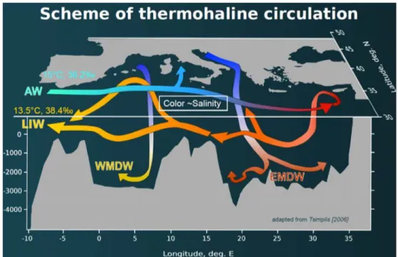
Figure 2: Sch´ema de la circulation thermohaline M´editerran´eenne. Modifi´e par L.Houpert de
Tsimplis et al. (2006). En anglais, AW= Atlantic Water, LIW=(Levantine Intermediate Water, WMDW=Western Mediterranean Deep Water, EMDW= Eastern Mediterranean Deep Water.
Le bassin m´editerran´een abrite environ 17 000 esp`eces et pr´esente un haut niveau ´elev´e d’end´emisme (Coll et al., 2010). La grande diversit´e des conditions climatiques a permis la coexistence d’esp`eces temp´er´ees et subtropicales (Bianchi and Morri, 2000). Les zones cˆoti`eres et les plateaux continentaux se caract´erisent par une biodiversit´e plus ´elev´ee, qui diminue g´en´eralement avec la profondeur (Coll et al., 2010). Bien qu’il s’agisse d’un haut lieu de la biodiversit´e, le bassin m´editerran´een est une zone oligotrophe en raison de l’afflux atlantique pauvre en nutriments et de l’exportation d’eau m´editerran´eenne riche en nutriments (Calvo et al., 2011).
La diversit´e et la richesse de l’environnement m´editerran´een a favoris´e le d´eveloppement d’une communaut´e multiculturelle le long de ses cˆotes. Depuis l’Antiquit´e, la mer M´editerran´ee a repr´esent´e une voie commerciale importante et le berceau de nombreuses civilisations qui ont
´
echang´ees et prosp´er´ees. Aujourd’hui encore, elle contribue de mani`ere significative au com-merce, `a l’´economie mondiale, ainsi qu’`a l’activit´e touristique. Toutefois, la mer M´editerran´ee est ´egalement une zone de conflit avec des tensions entre les usagers et une concurrence pour les ressources. Les villes cˆoti`eres associ´ees au 23 ´etats modernes sont dens´ement peupl´ees (500 millions d’habitants). Ces villes sont associ´ees `a de fortes diff´erences socio-´economiques et font face `a de multiples d´efis environnementaux et sociaux. Les conditions climatiques participent notamment au d´eficit en eau douce, `a l’augmentation du stress thermique et de la pollution qui affectent la sant´e, ainsi qu’`a une intensification des ´ev´enements extrˆemes (s´echeresses, inonda-tions, vagues de chaleur) qui affectent fortement les ´economies (Navara and Tubiana, 2013). Source de chaleur et d’humidit´e pour l’atmosph`ere, la mer M´editerran´ee contribue `a l’origine de aux ph´enom`enes m´et´eorologiques extrˆemes qui ont souvent lieu sur ses cˆotes et ont de graves cons´equences sur les populations. Elle fournit n´eanmoins un large ´eventail de services ´
ecosyst´emiques dont d´epend la qualit´e de vie des communaut´es et les activit´es ´economiques (Bleu, 2008). Par cons´equent, une strat´egie collective en termes d’observation, de surveillance et de gestion des ressources marines apparaˆıt n´ecessaire pour accroˆıtre la r´esilience des socio-´
ecosyst`emes m´editerran´eens dans un contexte de changement climatique.
Changement Climatique Futur en M´
editerran´
ee
Au cours du 21`eme si`ecle, un climat nettement plus chaud - plus que la moyenne mondiale - plus sec et avec une variabilit´e temporelle augment´ee a ´et´e envisag´e pour la r´egion m´editerran´eenne par plusieurs ´etudes de sc´enarios d’augmentation globale des ´emissions de gaz `a effet de serre (GES). La M´editerran´ee est donc souvent qualifi´ee de ≪point chaud≫ du changement clima-tique (Giorgi, 2006). Si l’´evolution de l’atmosph`ere du bassin au cours du 21`eme si`ecle a ´et´e largement document´ee, la r´eponse de la mer M´editerran´ee au changement climatique reste un sujet peu ´etudi´e jusqu’`a pr´esent. Par cons´equent, les multiples sources d’incertitude quant `a son ´evolution future sont encore moins connues. Les rares ´etudes existantes ont analys´e com-ment l’augcom-mentation des GES est susceptible de modifier les diff´erentes composantes de la mer M´editerran´ee. D’ici la fin du si`ecle, ces ´etudes indiquent : une r´eduction des pr´ecipitations allant jusqu’`a 35%, une augmentation de la perte nette d’eau `a la surface de la mer (par ex-emple,Adloff et al. (2015);Mariotti et al. (2008)), une diminution de la perte nette de chaleur en surface sur mer (par exemple, Somot et al. (2006, 2008); Dubois et al. (2012); Adloff et al.
(2015)), une augmentation de TSM de +1.5 °C `a +3 °C selon le sc´enario d’´emissions de GES, (par exemple,Somot et al.(2006,2008);Mariotti(2010);Adloff et al.(2015)) et une augmenta-tion possible de la salinit´e de surface (SSM). En raison des incertitudes associ´ees aux propri´et´es de la mer M´editerran´ee cit´ees pr´ec´edemment, l’´evolution future des ph´enom`eneses de forma-tion d’eau profonde et de MTHC es incertains. Par cons´equent, l’´evolution des caract´eristiques des eaux m´editerran´eennes sortant `a Gibraltar et leurs effets sur l’oc´ean Atlantique restent ´
Canicules Oc´
eaniques en mer M´
editerran´
ee
Au del`a de l’´evolution moyenne du climat en mer M´editerran´ee, plusieurs ´etudes montrent que les extrˆemes de temp´erature, de pr´ecipitation et de s´echeresse sont susceptibles de devenir plus fr´equents dans la r´egion au cours du 21`eme si`ecle (IPCC,2007;Planton et al.,2012b;Giorgi and Coppola, 2009;Hertig et al., 2010) . En particulier, on s’attend `a ce que le changement clima-tique augmente la fr´equence des ´episodes de chaleur extrˆeme de 200 `a 500% dans toute la r´egion durant le 21`eme si`ecle (Diffenbaugh et al.,2007). La concomitance de l’augmentation de la TSM attendue pour la mer M´editerran´ee devrait ´egalement acc´el´erer l’occurrence d’´ev´enements ther-miques extrˆemes en mer, appel´es Canicules oc´eanique ou Marine Heatwaves (MHW) en anglais. Ces ´episodes repr´esentent un r´echauffement anormal des oc´eans et ont montr´e lors des derni`eres d´ecennies de forts impacts ´ecologiques et des implications socio-´economiques impor-tantes (Hobday et al., 2016; Fr¨olicher and Laufk¨otter, 2018). Superpos´ees `a la tendance sous-jacente du r´echauffement de l’oc´ean, les MHW se produisent r´egionalement de l’´echelle de la cˆote au grand large, et peuvent modifier les ´ecosyst`emes marins en quelques semaines ou quelques mois seulement. Des r´eactions en chaˆıne ont ´et´e observ´ees entraˆınant l’effondrement de la pˆeche commerciale, de fortes pertes financi`eres et des tensions ´economiques entre les nations (Mills et al.,2013). Ces temp´eratures de la mer anormalement ´elev´ees peuvent persister dans le temps mais sont ´egalement susceptibles de s’´etendre dans l’espace. Bien que de tels ´ev´enements se soient probablement produits dans le pass´e sans avoir ´et´e d´etect´es, le r´echauffement de l’oc´ean les rend plus pertinents d`es lors que le stress thermique approche ou d´epasse les seuils de thermo-tol´erance de certains ´ecosyst`emes. L’am´elioration r´ecente des syst`emes d’observations et de t´el´ed´etection permet aujourd’hui de suivre l’´evolution spatio-temporelle de la surface de la mer tandis que l’augmentation du nombre de mesures in situ a r´ev´el´e l’extension en profondeur des MHW (Schaeffer and Roughan, 2017; Rose et al., 2012).
Nos connaissances actuelles sur les MHW pass´ees en M´editerran´ee se basent principalement sur l’identification d’´episodes de mortalit´es massives d’esp`eces benthiques li´ees `a des anomalies thermiques. Ces anomalies ont augment´e depuis le d´ebut des ann´ees 1990 (Rivetti et al.,2014;
Coma et al., 2009), bien qu’elles aient ´et´e observ´ees d`es les ann´ees 1980. L’un des premiers ´
ev´enements de grande ampleur document´e au niveau mondial s’est produit en mer M´editerran´ee en 2003, avec des anomalies de surface de 2 °C `a 3 °C au-dessus de la moyenne climatologique qui ont perdur´e pendant plus d’un mois. Cet ´ev´enement a entraˆın´e une mortalit´e massive d’invert´ebr´es benthiques, la disparition de prairies marines et des changements brusques dans la composition des communaut´es (Garrabou et al., 2001; Diaz-Almela et al., 2007). D’autres ´
episodes de mortalit´es massives associ´es `a des anomalies thermiques ont ´egalement ´et´e identifi´es au niveau r´egional dans le bassin en 1994 (Marb`a et al.,2015), 1999 (Perez et al.,2000;Garrabou et al.,2001), 2006 (Kersting et al.,2013;Marba and Duarte,2010), 2008 (Huete-Stauffer et al.,
2011; Cebrian et al., 2011), 2009 (Di Camillo et al., 2013; Rivetti et al., 2014) et 2010-2013 (Rodrigues et al.,2015). La plupart des ´episodes document´es ont touch´e des esp`eces corallig`enes (gorgones, ´eponges, herbiers de posidonie) jusqu’`a 50 m de profondeur (Rivetti et al.,2014) et `a quelques occasions entre 80 et 160 m (Arnoux et al.,1992;Rivoire,1991;Vacelet,1990). Jusqu’`a
pr´esent, les ´etudes se sont principalement concentr´ees sur les impacts ´ecologiques locaux, sans ´
evaluer syst´ematiquement l’occurrence des MHW.
Par cons´equent, un nombre d’´etudes encore plus r´eduit a port´e sur les m´ecanismes sous-jacents des MHW et leurs tendances futures dans le bassin. L’´evolution de la TSM m´editerran´eenne extrˆeme au 21`eme si`ecle a jusqu’`a pr´esent ´et´e examin´ee uniquement par rap-port aux r´eponses de thermo-tol´erance de certaines esp`eces. Par exemple, en utilisant un ensemble de mod`eles climatiques et le sc´enario A1B mod´er´ement optimiste pour les ´emissions de GES, Jord`a et al. (2012) ont sugg´er´e une augmentation de la mortalit´e des herbiers marins dans l’avenir autour des ˆıles Bal´eares en raison d’une augmentation pr´evue de la TSM maxi-male annuelle d’ici 2100. De la mˆeme mani`ere, Bensoussan et al.(2013) ont ´evalu´e le risque de mortalit´e de masse li´e au stress thermique dans les ´ecosyst`emes benthiques pour le 21`eme si`ecle, sur la base du r´echauffement moyen estim´e entre 2090-2099 et 2000-2010, selon le sc´enario pes-simiste du r´echauffement futur A2. Enfin, Galli et al. (2017) ont montr´e une augmentation de la fr´equence, de la s´ev´erit´e et de l’extension verticale des MHW en supposant des d´epassements des seuils de thermo-tol´erance sp´ecifiques aux esp`eces en utilisant le sc´enario `a fortes ´emissions RCP8.5 du GIEC. Plus r´ecemment,Oliver et al. (2018a) ont identifi´e une augmentation signi-ficative des MHW dans le monde au cours du si`ecle dernier (y compris en M´editerran´ee), tandis queFr¨olicher et al.(2018) ont pr´evu une augmentation des MHW dans le monde pour le 21`eme si`ecle.
Motivation de l’´
etude
Il est ´evident que sous l’effet continu du r´echauffement climatique anthropique, les oc´eans de la plan`ete deviennent de plus en plus sensibles aux ´ev´enements thermiques extrˆemes. Compte tenu de la sensibilit´e du bassin m´editerran´een au changement climatique, une ´etude plus appro-fondie de sa vuln´erabilit´e et de la r´eponse des MHW apparaˆıt n´ecessaire. Cette th`ese s’inscrit dans cet objectif et tente de fournir une ´evaluation robuste de l’´evolution des MHWS estivales m´editerran´eennes dans le pass´e, le pr´esent et le futur en d´eterminant comment d´efinir une MHW, quand et o`u surviennent-elles et quels sont leurs facteurs explicatifs.
Par ailleurs, la compr´ehension actuelle de la r´eponse de la mer M´editerran´ee au changement climatique futur repose principalement sur des ensembles de mod`eles climatiques de circulation g´en´erale `a faible r´esolution spatiale (CMIP5) (Jord`a et al., 2012; Mariotti et al., 2015) ou sur des exp´eriences num´eriques r´ealis´ees avec un mod`ele oc´eanique r´egional unique et utilisant tr`es rarement plusieurs sc´enarios d’´emission (Somot et al., 2006; Bensoussan et al., 2013; Adloff et al., 2015; Galli et al., 2017; Macias et al., 2018). Par cons´equent, les ´etudes publi´ees dans la litt´erature avec des mod`eles adapt´es `a la mer M´editerran´ee ne tiennent pas bien compte des diff´erentes sources d’incertitude, (i) au choix du mod`ele climatique et (ii) `a la variabilit´e chaotique naturelle. Par contre, il y a quelques ´etudes que ils ont tenues compte l’ incertitude associ´ees au choix du sc´enario socio-´economique (par exemple,Adloff et al.(2015)). Cependant, les ´etudes d’impact du changement climatique sur les ´ecosyst`emes m´editerran´eens et les activit´es maritimes sont le plus souvent bas´ees sur une seule simulation climatique et ne peuvent donc
pas ˆetre consid´er´ees comme robuste.
Par cons´equent, un autre objectif de cette th`ese est d’aborder ces incertitudes. Nous con-sid´ererons pour cel`a diff´erents futurs climatiques possibles par le biais d’une approche multi-mod`ele et multi-sc´enario tenant compte de la variabilit´e chaotique, en utilisant pour la premi`ere fois un ensemble d´edi´e de mod`eles coupl´es et haute r´esolution du syst`eme climatique r´egional (Regional Climate System Model, RCSM, en anglais).
Dans le contexte du r´echauffement climatique, l’estimation `a long terme des caract´eristiques spatiales des MHW pourrait aider `a identifier les r´egions ayant une pr´edisposition au d´eveloppement de ces ´ev´enements extrˆemes. La M´editerran´ee regroupe sur une faible superficie de nombreux risques tels que les s´echeresses, la modification de la biodiversit´e, la croissance d´emographique, les migrations et les conflits. Une meilleure connaissance des risques li´es aux MHW dans cette r´egion apparaˆıt donc essentielle afin d’assurer la durabilit´e des communaut´es qui d´ependent de la mer. L’utilisation d’un algorithme automatique de detection et de descrip-tion des MHW s’av`ere donc utile pour les syst`emes de suivi et de pr´evision mais ´egalement pour la diffusion de l’information permet le d´eveloppement de strat´egies de gestion efficaces de ces ´ev´enements. La m´ethode d´evelopp´ee dans le cadre de ce travail de th`ese s’applique aux ´
ev´enements estivaux uniquement et est disponible en libre acc`es pour les utilisateurs int´eress´es (industries de la pˆeche, centre de pr´evision).
Le chapitre 1 du pr´esent manuscrit propose une introduction concernant la r´egion m´editerran´eenne, son climat et les connaissances actuelles sur les MHW. Le d´eveloppement original d’une m´ethode de d´etection automatique des MHW estivales en M´editerran´e est d´ecrite dans le chapitre 2, ainsi qu’un exemple de son application sur la canicule oc´eanique bien connue de 2003 dans le bassin. Le chapitre 3 est propos´e sous la forme d’un article prˆet `a ˆetre soumis et pr´esente l’´etude des MHW m´editerran´eennes pass´ees ainsi que de leurs caract´eristiques sur la p´eriode 1982-2017 avec une analyse des m´ecanismes explicatif. Le chapitre 4 se compose d’un article en r´evision qui traite de l’´evolution spatio-temporelle des MHW au cours du 21`eme si`ecle. Une analyse des incertitudes entourant les caract´eristiques des ´ev´enements au 21`eme si`ecle est effectu´ee `a l’aide d’un ensemble de mod`eles coupl´es `a haute r´esolution et de diff´erents sc´enarios d’´emissions de GES. Enfin, les conclusions et perspectives de ces travaux de th`ese font l’objet de la derni`ere partie du manuscrit, ainsi qu’une annexe sur le mat´eriel compl´ementaire de ces travaux.
2.1 Differences between the characteristics of CNRM-RCSM4 and CNRM-RCSM6 models. . . 49
2.2 Basin-mean, yearly-averaged (SST ) and extreme (SSΤ99Q) temperatures (°C) and their trends (°C/year) over the period 1982-2012. Values are shown respec-tively for CNRM-RCSM6, CNRM-RCSM4 and a satellite dataset interpolated at each different grid every time.. . . 52
2.3 Correlation Coefficient between CNRM-RCSM6, CNRM-RCSM4 and
observa-tions. With OBS is denoted the respective interpolated observations for each model. Pattern correlations are performed, using the Pearson product-moment coefficient of linear correlation between two variables. For the timeseries, the Pearson sample linear cross-correlation at lag 0 only was used. Correlations were performed with ncl software. . . 53
2.4 Marine Heatwave (MHW) set of properties and their description adapted from (Hobday et al., 2016) . . . 61
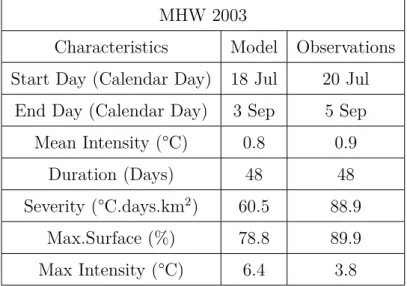
2.5 Average, characteristics of MHW 2003 throughout the event duration. Starting and ending day (calendar day), duration (Number of days), mean and maximum intensity (°C), severity*106 (°C.days.km2) and maximum surface coverage (%) are presented for both the model and the satellite observations. . . 62
2.6 Sensitivity experiments on the MHW 2003 characteristics using MHW definitions with different baseline thresholds. Units are as in Table.2.5. Reference definition is indicated with bold. See text for more details. . . 66
2.7 As in Table.2.6 but for MHW definitions with changes on gap day number, spatial threshold and minimum event duration. See text for more details. . . 68
3.1 Basin-mean, extreme temperature evolution at surface SST99Q and at depth
T99Q over 1982-2017. Shown here also, are the domain-averaged mean surface and subsurface MHW frequency, Imean, Duration, Severity (Icum), Surfmax and Imax and error bar at 95% confidence level for every layer. Linear trends of domain-averaged timeseries with statistical significance higher than 95% level are indicated in bold. . . 80
3.2 Marine Heatwave characteristics at the Mediterranean Sea surface as identified from the satellite dataset during 1982-2017. Here shown are, Starting day (calen-dar day), Ending day (calen(calen-dar day), Imean (°C), surfmax (%), duration (Days), Severity*106 (°C.days.km2) and Imax (°C) of every event separately. . . 86
3.3 As in Table.3.2 but for surface MHWs identified from the model during 1982-2017. 87
3.4 As in Table.3.3 but for MHWs identified from the model at 23m during 1982-2017. 88
3.5 As in Table.3.3 but for MHWs identified from the model at 41m during 1982-2017. 89
5.1 Characteristics of the coupled Regional Climate System Models (RCSM) and the simulations used in this study. More information on MEDATLAS initial conditions can be found in Rixen et al. (2005). . . 119
5.2 Marine Heatwave (MHW) set of properties and their description after Hobday et al. (2016) . . . 123
5.3 Evaluation of SST and MHW properties during HIST run. Mean annual and threshold SST are indicated with SST (°C) and SST99Q (°C) respectively. The Mann-Kendal parametric test is used to detect the presence of linear or non-linear monotonic trends (°C/year) in domain-averaged SST timeseries. Trends with statistical significance lower than 95% level are indicated with star. Spatial correlations (Corr.Coeff) and bias with respect to observations are given for each dataset. Also shown here, are the range (min and max) of frequency, duration (days), starting day (calendar month), ending day (calendar month), Imean (°C) Imax (°C), Severity*107 (°C.days.km2) and maximum surface coverage(%) of MHWs. The multi-model column indicates the ensemble average values and standard deviation for each variable. . . 127
5.4 Future Mediterranean-averaged, yearly mean (SST ) and extreme (SST99Q) anomalies (with respect to HIST) for the near and far future under different emission scenarios. The multi-model column indicates the ensemble average val-ues and standard deviation. Valval-ues are in °C. . . 129
5.5 Future response (anomalies with respect to HIST) of MHW mean properties for the 6 RCSMs under RCP8.5, RCP4.5 and RCP2.6, for the near (2021-2050) and far future (2071-2100). Shown here are the average annual event count (fre-quency), average MHW duration (days), starting day (calendar month), ending day (calendar month), Imean (°C), Imax (°C), severity (*107°C.days.km2) and maximum surface coverage (%). The multi-model column indicates the ensemble mean values for each variable and their standard deviation. Only the CNRM simulation is available for the RCP2.6 scenario, 5 simulations for RCP8.5 and 5 simulations for RCP4.5. . . 133
5.6 Anomalies of future MHW characteristics with respect to HIST run (climate change response) using different MHW definitions. Calculations are performed only for the CNRM model for the period 2071-2100 of the RCP85 scenario. First columns display MHW definitions with different SST thresholds (e.g 90th quan-tile of SST, 95th quanquan-tile of SST etc.). Climate change response of MHWs when the mean SST difference between HIST and 2071-2100 is added to the original
SST99Qthreshold is also showed in column 9. Further definitions are also tested: EXP.1 is an experiment performed without gap days on the MHW definition but the 20% spatial threshold retained. EXP.2 refers to MHWs detected with a definition that allowes 2 gap days and a minimum spatial threshold of 20%. In EXP.3 MHW definition allows up to 5 cool days that are lower than the initial threshold by up to 0.3 °C and a minimum spatial threshold of 20%. EXP.4 uses a MHW definition where gap days are defined as described in this paper but there is a 10% minimum limit on spatial threshold. Finally, Exp.5 and Exp.6 are tests of MHW definition where minimum duration of the events is set at 3 days and 7 days respectively. By MHW definition is implied the definition used in the paper with a spatial threshold of SST99Q. . . 141
5.7 SST properties during 1982-2005 years of HIST run and the observations. Mean annual and threshold SST are indicated with SST and SST99Q. The mann-Kendal parametric test is used to detect the presence of linear or non-linear trends (°C/year) in domain-averaged SST timeseries. Spatial correlations (Corr.Coeff) and bias with respect to observations are given for each model dataset.141
1 R´egion m´editerran´eenne et ses sous-bassins. Circulation des eaux de surface est ´egalement illustr´ee (redessin´ee d’apr`es De Madron et al. (2011)). Les vents saisonniers et regionaux sont indiqu´es par des couleurs et leurs noms entre par-enth`eses. Modifi´e par S.Darmaraki. Credits: Frank Ramspott . . . vi
2 Sch´ema de la circulation thermohaline M´editerran´eenne. Modifi´e par L.Houpert de Tsimplis et al. (2006). En anglais, AW= Atlantic Water, LIW=(Levantine Intermediate Water, WMDW=Western Mediterranean Deep Water, EMDW= Eastern Mediterranean Deep Water.. . . vii
1.1 Mediterranean region and its subbasins. Circulation of surface water masses is also illustrated (redrawn from De Madron et al. (2011)). Seasonal, regional winds are indicated with colours and their names in parenthesis.Modified by S.Darmaraki. Credits: Frank Ramspott . . . 3
1.2 Schematic of Mediterranean Thermohaline Circulation. Modified by L.Houpert from Tsimplis et al. (2006). AW=Atlantic Water, LIW=(Levantine Interme-diate Water, WMDW=Western Mediterranean Deep Water, EMDW=Eastern Mediterranean Deep Water) . . . 4
1.3 Figure representing the minimum domain prescribed for the representation of the Mediterranean area, by the for the Med-CORDEX ensemble of models. . . . 7
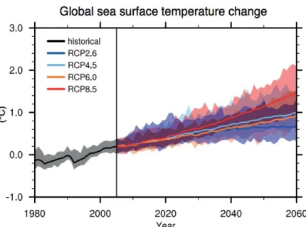
1.4 Projected changes in annual averaged, globally averaged, surface ocean temper-ature based on 12 Atmosphere–Ocean General Circulation Models (AOGCMs) from the CMIP5 multi-model ensemble, under 21st century scenarios RCP2.6, RCP4.5, RCP6.0 and RCP8.5. Shading indicates the 90% range of projected an-nual global mean surface temperature anomalies. Anomalies computed against the 1986–2005 average from the historical simulations of each model.(Kirtman et al., 2013). . . 8
1.5 Example of the sources of uncertainty in global decadal temperature projections. Each coloured area corresponds to a different contribution, representing a 90% confidence interval (Kirtman et al., 2013). . . 9
1.6 Summer, surface air temperature anomalies over the period 1860-2098 relative to 1980-2005, averaged over the Mediterranean land area only, from an ensemble of CMIP5 by (Mariotti et al., 2015). Ensemble mean temperatures (°C) are indicated in red, individual model simulations in grey and observational datasets in black, blue and yellow. Red triangle at the top of each graph indicate the years with major volcanic eruptions while vertical dash line in 2005 separates historical run from future projections . . . 10
1.7 Mediterranean Sea area-averaged anomalies of the Evaporation - Precipitation (left) and the total freshwater deficit (right) for the period 1950-2100 relative to 1950-1999 from Regional Climate System Models, taken from Sanchez-Gomez et al. (2009). The black line represents the multi-model ensemble mean filtered to remove period shorter than 5 years. The coloured shading indicates uncertainty interval for the 90% level. . . 12
1.8 Basin-mean, yearly-averaged sea surface temperature anomalies between 1960-2100 relative to 1961-1990, by Adloff et al. (2015), using the regional ocean model NEMOMED8 and an ensemble of different socio-economic scenarios, based on the Special Report on the Emisson Scenarios. Spread of the ensemble is indicated in grey, while A2-F, A2-RF and A2-ARF curves are overlapping. . . 14
1.9 Same as Fig.1.8 but for sea surface salinity. . . 15
1.10 As in Fig.1.6 but for the area-average SST over the Mediterranean Sea. Obser-vational SST is from the HadISST dataset (black line). Adapted from Mariotti et al. (2015). On the contrary to Fig.1.8, this is the SST spread given from an ensemble of GCM models. . . 15
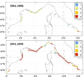
1.11 Impact mapping on the risk of mortality outbreak for Paramuricea clavata at the beginning (Top) and end (Bottom) of the 21st century along the continental coastal stripe north of 39 °N in the NW Mediterranean Sea. The colour scale, from 1 to 4, corresponds to sub-lethal, moderate, high and extreme lethal impacts respectively (Bensoussan et al., 2013) . . . 19
1.12 Chain of Regional Climate Modeling . . . 20
1.13 Examples of prominent MHWs that have occurred recently and have been an-alyzed in the literature. Maximum sea surface temperature anomaly above re-gional 99th percentile is indicated here, using the NOAA Optimum interpolation sea surface temperature dataset. Reference period is 1982-2016. Image taken from Fr¨olicher and Laufk¨otter (2018). . . 24
1.14 SST anomaly of May 2015 with respect to 2002-2012 climatology shows the ”Pacific Blob”. (Map by American Geophysical Union) . . . 26
1.15 Most prominent MHWs during the last decade and their driving mechanisms. Credits, Eric Oliver, Dalhousie University.http://www.marineheatwaves.org . . . 29
1.16 Schematic of MHW definition by Hobday et al. (2016) . . . 30
1.17 Schematic of MHW classification by Hobday et al. (2018) . . . 31
1.18 Difference of MHW properties between 1982-1998 and 2000-2006 (b,e,h) and their respective globally-averaged annual mean timeseries (c,f,i) with (black) and without (red) ENSO effect. Hatching denotes that the difference is statistically significant at the 5% level while red and blue denote El Ni˜no and La Ni˜na periods respectively. Figure taken from Oliver et al. (2018a). . . 33
1.19 Simulated changes in MHW probability of occurence (top left), mean inten-sity(down left), duration (top right) and spatial extent (down right) for different levels of global warming. Figure taken from Fr¨olicher et al. (2018). . . 35
1.20 Examples of MHW impacts on marine ecosystems. Coral bleaching (top left) and sea grass die-off (top right) are indicated, along with mass mortality of abalone (down left) and changes in recruitment patterns of lobsters (down right). Severe ecological and socio-economic consequences accompanied these abrupt changes . 36
1.21 Summer Marine Heatwaves in the Mediterranean Sea during the last two decades, as they have been reported by bivalve mollusc producers from 12 coastal regions of 6 Mediterranean countries. The figure is adapted from Rodrigues et al. (2015) and is part of a questionnaire for the environmental threats encountered by the representatives of the aquaculture sector in the Mediterranean basin. . . 39
1.22 Comparison between observed and simulated MHW trends in the northeastern Mediterranean Sea. Linear trends in MHW (A) frequency, (B) duration and (C) intensity are shown as a funtion of linear trend in annual mean SST. Grey lines correspond to a 1000-member ensemble of simulated SSTs using a stochastic climate model and assuming only linear changes in the annual mean SST. The ensemble mean and 2.5th and 97.5th percentile are shown in black, blue and red lines respectively. White circle denotes the observed MHW property trends situated on the x axis, according to the observed trend in annual mean SST. Figure adapted from Oliver et al. (2018a). . . 40
1.23 Maximum number of consecutive days above 30°C for 2001-2010 (A,C,E,G) and between 2041-2050 under RCP8.5 (B,D,F,H) at different depths. Colormap is scaled to highlight a specied-specific 20-day lethal threshold. Magenta dots are locations of mussel farming facilities. . . 41
1.24 An example of 21st century projections of the annual maximum SST but averaged over the Balearic islands area. The output from 10 AOGCMs is indicated in grey, of an RCSM in purple and of an ocean-standalone RCM in blue, while the ensemble mean in red. Figure is produced by Jord`a et al. (2012) . . . 42
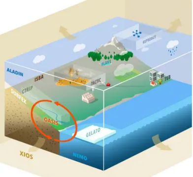
2.1 Schematic of the components of the CNRM-RCSM6 model. Credits: CNRM . . 47
2.2 The extended Mediterranean domain covered by the CNRM-RCSM6 model. To-pography, bathymetry and land-sea mask are illustrated, while the ocean and Black Sea (which are not included in the NEMOMED12) are in white. Cred-its:Nabat Pierre personal communication. . . . 48
2.3 Land-sea mask orography (ALADIN-Climate) and NEMOMED8 bathymetry for
the MED-CORDEX domain of CNRM-RCSM4. Drainage area of Black and Mediterranean Sea are contoured in black and red respectively. Figure from Sevault et al. (2014). . . 49
2.4 Average of yearly mean SST (°C) during 1982-2012 for CNRM-RCSM6 and
CNRM-RCSM4 in hindcast mode and satellite data interpolated at each respec-tive grid. . . 50
2.5 As in Fig.2.4 but for SSΤ99Q. . . 51
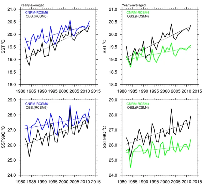
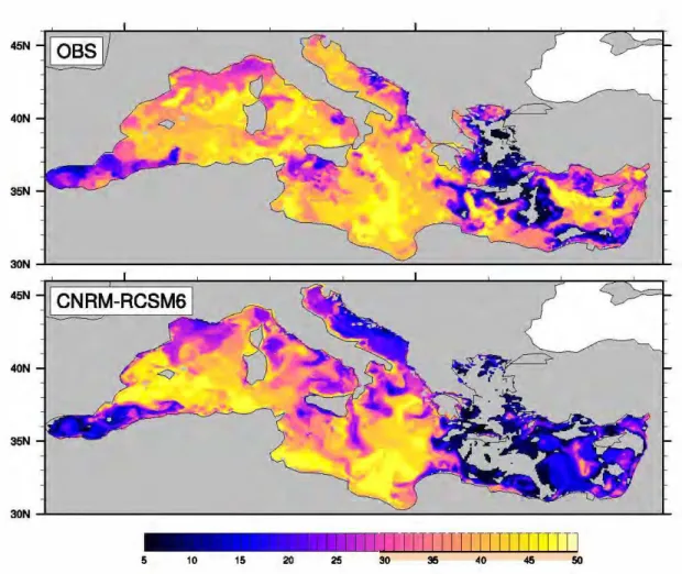
2.6 Yearly SSΤ99Q (°C) during 1982-2012 for CNRM-RCSM6 and CNRM-RCSM4
in hindcast mode. Shown here is also average SSΤ99Q for the same period from the satellite dataset interpolated at each respective grid. . . 52
2.7 Flow chart for the grid-based detection of a summer Mediterranean MHW. Light blue rhombus refers to the detection of the starting, warm and ending day of an event, while light red signifies the part of the program where gap days are identified and treated. Dark blue rhombus represent the condition under which an event is interrupted entirely without counted as a MHW. Black line denotes the average SST over the days it comprises. . . 56
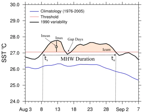
2.8 Schematic of a MHW based on Hobday et al. (2016). The black line represents daily SST variations of one grid point in a random year, red line is the local threshold (SST99Q) and blue line is the daily 30-year climatology for this point. Also shown here also are the starting day (ts) and ending day (te) above SST99Q, gap days and the different measures of daily intensity (see text for more details). MHW metrics refer to the total event duration. . . 57
2.9 Example of the MHW(s) detected during 2003 at 2 specific, NW-Mediterranean grid points, by applying the algorithm on CNRM-RCSM6 (blue), satellite (green) and in situ (black dotted) data correspondingly. For each dataset, daily SST variability is displayed along with the corresponding SST99Qthreshold line. The starting and ending day identified by each dataset is also shown within the grey area enclosed by the corresponding, in color, dashed vertical lines. . . 58
2.10 Example of the daily mean intensity of the MHW during the event of 2003, as detected by our algorithm, using the CNRM-RCSM6 in hindcast mode. Evolu-tion of MHW area is illustrated in selected days and not throughout the entire duration of the event. Areas that were not affected by the MHW are indicated in dark blue. . . 60
2.11 Daily MHW area summed over the basin every year between 1982-2012 and expressed in percentage of the Mediterranean Sea surface coverage in km2, using the original MHW definition (Q99). Spatial threshold of 20% is indicated with dash line. . . 61
2.12 Bubble graph of MHW 2003 for both the model (NEMOMED12) and the satel-lite observations (OBS). Duration is in number of days, mean intensity in °C, severity*106 in °C.days.km2 and maximum surface coverage in %. . . 63
2.13 Mean intensity (°C) of the MHW 2003 throughout the event duration, as it was captured from the detection algorithm using CNRM-RCSM6 and satellite observations. Gray ocean areas represent grid points not affected by the MHW. 64
2.14 As in Fig.2.13 but for the total number of days touched by the MHW at every grid point. . . 65
2.15 Bubble graph representing the characteristics of the MHW 2003, based on dif-ferent experiments on the MHW definition. Color scale corresponds to severity (*106°C.days.km2) and size of the bubbles to percentage of maximum surface coverage (surfmax) of the MHW. See the text for more details. . . 67
2.16 As in Fig.2.15 but with the observed MHW 2003 (bubble with bold circle, less opaque) superimposed on the simulated MHW (bubble more opaque and no bold circle). . . 69
2.17 Number of summer Mediterranean MHWs per year during 1982-2012 identified by CNRM-RCSM6 (top left), CNRM-RCSM4 (bottom left) and observations interpolated in CNRM-RCSM6 grid (top right) and CNRM-RCSM4 grid (bottom right). . . 70
2.18 IDF plot for the MHW characteristics identified by RCSM6, CNRM-RCSM4 and the observations interpolated in the respective grids for 1982-2012. 71
3.1 (top) Threshold maps (SST99Q,T99Qover 1982-2012), for the observations (a) and the model at surface (b) and at depth (23m (c), 41m (d), 55m (e)). (bottom) Annual, basin-mean observed and simulated SST99Q and T99Q trends for 1980-2017 for the different layers. . . 78
3.2 Individual MHW characteristics at surface and different depths (a-e). Color scale corresponds to severity (*106°C.days.km2) and size of the bubbles to surfmax. Daily average surfmax for 1982-2017 is also depicted (f) at different layers in relation to event timing. . . 81
3.3 Average MHW Imean (°C) (top) and duration (days) (bottom) over 1982-2017, for the observations and the model, normalised by the number of event at each layer. . . 83
3.4 Difference between the characteristics of each subsurface MHW and its corre-sponding preceding surface event of a given year, versus the properties of the surface MHW. For every plot, the total number of individual subsurface MHWs identified throughout the period examined are pooled, independently from the depth where they occurred. . . 91
4.1 Schematic of the processes that act on the time-rate of temperature change. Based on Holbrook et al. (subm). . . 93
4.2 Mixed Layer (a-d) and atmosphere (e-h) heat budget decomposition 7 days be-fore, during and 7 days after the Mediterranean MHW 2003. MHW period is displayed between dashed lines. Each term’s daily timeseries is averaged over the MHW area and is shown in absolute values (a,c,e,g) and in anomalies (b,d,f,h) with respect to 1982-2017 climatology. See text for more details. . . 98
4.3 Schematic of the Mediterranean Sea separation in subbasins. The different areas are displayed with their acronyms as defined in text. On the background the spatial distribution of the mean intensity (°C) during the MHW 2003. See text for more details. . . 101
4.4 Daily timeseries of a)SST and ML temperature (Temp) anomalies, b) MLD anomalies, c) ML heat budget terms in absolute values, d) Anomalies of ML heat budget terms, e) Windspeed anomalies, f) 2m-air temperature anomalies, g) Atmosphere heat budget terms in absolute values, h) Atmosphere heat budget terms in anomalies, for the Gulf of Lion (GOL). Values are averaged for 7 days before, during and 7 days after the MHW 2003. . . 103
4.5 As in Fig.4.4 but for the Ionian Sea domain. . . 104
4.6 As in Fig.4.4 but for the Tyrrhenian Sea domain. . . 105
4.7 As in Fig.4.4 but for the Algerian Sea domain. . . 106
4.8 As in Fig.4.4 but for the Gulf of Gabes domain. . . 107
4.9 SST and ML temperature anomalies (left column) and MLD anomalies (right column) for every EMED subbasin, 7 before, during and 7 days after the MHW. 109
4.10 Absolute (a-f) and anomalous values (g-l)for the different MLD heat budget terms, 7 days before, over the event duration and 7 days after the MHW. . . 110
4.11 As in Fig.4.10 but for the atmosphere heat budget terms. . . 111
4.12 As in Fig.4.9 but for windspeed and 2m-air temperature anomalies. . . 112
5.1 Schematic of a MHW based on Hobday et al. (2016). The black line represents daily SST variations of one grid point in a random year and red line is the local threshold (SST99Q) based on the 30-year average of the yearly 99th quantile of daily SST for that point. The blue line is the daily 30-year climatology for this point. Also shown here also are the starting day (ts) and ending day (te) above SST99Q, gap days and the different measures of daily intensity. MHW metrics refer to the total event duration.. . . 122
5.2 Yearly SST (°C) for the HIST run of every model (1976-2005) and satellite data during 1982-2012. Note that the HIST run for ENEA is from 1979-2005. . . 124
5.3 Individual MHW threshold maps of mean SST99Q(°C) computed from the HIST run of every model (1976-2005) and satellite data during 1982-2012. Note that the HIST run for ENEA is from 1979-2005 . . . 125
5.4 Timeseries of area-averaged, yearly SST °C (left) and SST99Q°C (right), during HIST for every model and satellite data, represented by a solid line. Trends are indicated in dashed lines. The different simulations are represented by different colors. . . 126
5.5 IDF plot; Intensity (Imean in °C), Duration (Days), Frequency (Number of MHW during 1976-2005). Imean is organised in bins of 0.02 °C, while dura-tion is in bins of 5, 10 and 20 days. Red box indicates observed characteristics corresponding to the exceptional MHW of 2003. . . 127
5.6 Area-average, yearly SST °C (left) and extreme SST99Q°C (right) anomalies with respect to HIST. Bold colors represent the multi-model average and lighter colors are the individual simulations. RCP2.6 scenario has only one simulation (CNRM), HIST run is illustrated in grey and observations in dashed black. . . . 128
5.7 Multi-model average anomaly of yearly SST (°C) with respect to the corre-sponding ensemble mean HIST of each scenario, for the near and far future. The RCP2.6 scenario has only one simulation (CNRM). . . 130
5.8 Multi-model average anomaly of extreme SST99Q (°C) with respect to corre-sponding ensemble mean HIST (1976-2005) of each scenario, for the near and far future. The RCP2.6 scenario has only one simulation (CNRM). . . 130
5.9 Annual number of MHWs (Annual Frequency) for RCP8.5 (red) RCP4.5 (blue) RCP2.6 (green) HIST (grey) and observations (dashed black). Bold colors indi-cate the multi-model mean and shaded zones represent individual MHW events identified by the models. Years without MHWs are also included, with shaded areas reaching 0. RCP2.6 has only 1 simulation (CNRM).. . . 131
5.10 Annual earliest starting (solid lines) and latest ending (dashed lines) day of MHW events for RCP8.5 (red) RCP4.5 (blue) RCP2.6 (green) HIST (grey) and observations (black). Bold colors indicate multi-model average values, while lighter dots represent individual event dates. . . 132
5.11 IDF (Imean, Duration, Frequency) plots display the total number of every dataset for every scenario over 2021-2050 and 2071-2100. RCP8.5 and RCP4.5 include events from 5 simulations, while RCP2.6 from only 1 (CNRM) simu-lation. HIST run contains MHWs from the corresponding set of models each time. The number of MHWs is calculated over each 30 year period. For contrast purposes, the red box depicts the observed characteristics of MHW 2003 in the Mediterranean. . . 134
5.12 Whisker diagram of (left) Severity (Icum) and (right) maximum surface coverage of every observed and simulated MHW during HIST, 2021-2050 and 2071-2100. Box plots illustrate minimum, 25th percentile, median, 75th percentile and max-imum values of each variable for a given model, scenario and period. . . 135
5.13 Multi-model mean ratio R of ∆ SST99Q (°C) over ∆ SST (°C) for every pe-riod and scenario. Regions where R>1/R<1 indicate regions where flatten-ing/narrowing of SST distribution is detected in addition to the mean distri-bution shift. Where R∼1 the SST increase can be considered as the main factor for MHW changes . . . 138
5.14 SST (°C) bias in relation to MHW characteristics anomalies of RCP45 (star) and RCP85 (circle) for both 2021-2050 and 2071-2100 periods, with respect to HIST run. For every variable model colors are represented as in main text. . . . 142
Introduction
”An adult scientist is a kid who never grew up.”
Neil deGrasse Tyson
Contents
1.1 The Mediterranean Region. . . . 2
1.2 Modeling of the Mediterranean Climate System . . . . 6
1.3 Climate Change Scenarios and Uncertainty. . . . 7
1.4 Projections for the Mediterranean Region . . . . 9
1.4.1 Mean Climate. . . 9
1.4.2 Future evolution of Mediterranean Sea Characteristics . . . 10
1.4.3 Impacts on Marine Ecosystems . . . 17
1.4.4 Uncertainties in Mediterranean Future Projections . . . 19
1.4.5 Climate Extremes in the Mediterrranean. . . 22 1.5 Marine Heatwaves . . . . 23
1.5.1 Driving Mechanisms . . . 24
1.5.2 Detection Methods . . . 30
1.5.3 Trends in the Past and the Future . . . 32
1.5.4 Impacts on Marine Ecosystems . . . 36
1.5.5 Subsurface Marine Heatwaves . . . 37
1.5.6 Marine Heatwaves in the Mediterranean Sea . . . 38 1.6 Conclusions . . . . 42
1.6.1 Motivation of the study . . . 42
1.1
The Mediterranean Region
Mediterranean area is a transitional, semi-enclosed basin formed between the temperate zone to its north and the subtropical zone to its south and east. Therefore, mid-latitude and tropical variability influence a complex topography of sharp mountains and mild coasts, permanent glaciers on the north and desert areas on the south, creating a highly responsive region to climate change. The area features mild and wet winters and a mostly warm or dry summer season. Its southeastern part is exposed to the Asian Monsoon during the warm months, while it remains under the influence of the descending branch of Hadley cell for most of the year (Lionello et al., 2012). Northern regions, however, are strongly linked to mid-latitude teleconnection patterns, such as NAO (North Atlantic Oscillation), EA (East Atlantic pattern) and others, associated with moisture transport from the North Atlantic (Xoplaki,2002;
Xoplaki et al.,2003). As a result, strong contrasts in temperature and precipitation behaviour arise within the basin, distributing temperate, arid but also mountain climates throughout its surface. These spatiotemporal patterns are also affected by the location of the basin at the limit of the North Atlantic storm tracks.
To its west, the Mediterranean Sea connects to the Atlantic Ocean through the straits of Gibraltar and to its northeast, through the Bosphorus Strait to the Black Sea (main freshwater inflow for the east basin). Connection with the Red Sea and the Indian Ocean is also estab-lished, through the Suez Canal. Meanwhile, the ten largest rivers discharging in the basin (e.g. Nile, Po, Ebro, Rhone, etc.) account for about half the average river input in the Mediterranean (Ludwig et al., 2009). The complicated land-sea patterns divide the Mediterranean Sea into smaller subbasins, such as the Ionian, Tyrrhenian, Aegean, Adriatic, Alboran, Balearic and Ligurian Sea. The shallow Straits of Sicily (∼ 400m) geographicaly separate the warmer and more saline eastern Mediterranean (EM) from the relatively colder and fresher, western Medi-terranean (WM) subbasin, throughout which, a major cyclonic (mostly) circulation is shaped (Fig.1.1).
It is a unique and active thermohaline circulation (MTHC) driven by heat and water losses at the sea surface (W¨ust,1961). An anti-estuarine circulation is formed based on the exchange between a relatively fresh and warm surface inflow from the Atlantic (36.2 psu, 15.4°C), which spreads and sinks towards EM transforming into a relatively cool and saltier Mediterranean water (38.4 psu, 13°C) that then outflows in an intermediate layer at the narrow Strait of Gibraltar (∼14.5 km) (Millot and Taupier-Letage, 2005). This very saline outflow may have a role to play in stabilizing the global THC (Thorpe and Bigg, 2000; Potter and Lozier, 2004;
Curry et al., 2003; Reid, 1979). The main flow is further sustained by winter-time deep-water formation (DWF) processes that occur in the Gulf of Lion, Adriatic, the south Aegean and northeast Levantine basin, due to evaporation and cooling induced by cold and dry regional winds (e.g. Mistral) (Schroeder et al., 2012). It is one of the few places in the world where convection cells, analogous to the polar Atlantic ones, are formed and ventilate intermediate
and deeper ocean layers (Malanotte-Rizzoli et al., 2014). The vertical mixing that takes place provides oxygen to deeper Mediterranean waters but also enriches surface waters with nutrients (Auger et al.,2014) that favor marine ecosystems (Fig. 1.2).
Gibraltar Ionian Levantine Black Sea Suez Canal Red Sea (Scirocco) (Mistral) (Bora) (Etesians) .
Figure 1.1: Mediterranean region and its subbasins. Circulation of surface water masses is also illustrated (redrawn from De Madron et al. (2011)). Seasonal, re-gional winds are indicated with colours and their names in parenthesis. Modified by S.Darmaraki. Credits: Frank Ramspott, https: // fineartamerica. com/ featured/ mediterranean-sea-3d-render-topographic-map-color-frank-ramspott. html
Unlike the global ocean conveyor belt, MTHC is a much smaller in size and timescale (∼100 years) open cell, which balances the excess of evaporation over the Mediterranean Sea, expressed through a net buoyancy flux towards the atmosphere (Lionello et al.,2012). Vertically, however, it forms 3 distinctive water masses that span the whole basin: The Atlantic water (AW) occupying a surface layer approximately between 100-200m, the Levantine Intermediate Water (AW) approximately between 300-800m and the Deep Water that extents to the bottom (∼5.267m). Internal thermohaline cells exist in the western and eastern subbasins, which are endowed with well-known boundary currents, jets that bifurcate, mesoscale eddies and gyres (Robinson et al., 2001), some of which are wind-driven (Amitai et al., 2010; Rinaldi et al.,
2010). Continental shelves, on the other hand play a significant role, since they constitute 20% of the total Mediterranean Sea surface, relative to a corresponding 7.6% of the global ocean (Pinardi et al., 2006). Its orographic surroundings and small-scale islands induces a highly diverse, regional and seasonal wind regime (e.g. Mistral, Meltemi, Sirocco, Tramontane, Bora), generating strong air-sea interactions that affect dense-water formation, MTHC and major
Mediterranean Sea features through latent heat and evaporation transfer (e.g. Romanou et al.,
2010). As a source of heat and moisture for the atmosphere, the Mediterranean Sea prompts the development of extreme weather events, with often severe consequences for the surrounding communities.
Although the region accounts for 0.32% of the global ocean volume, it hosts approximately 17000 species and a high level of endemism (Coll et al., 2010). A variety of different habitats is developed in its coastal lagoons, salt marshes, estuaries, deltas, rocky and sandy coastlines, sea grass and coralligenous beds, canyons, plateaux and undersea mountains, favoring the di-versity of organisms (Benoit, 2006). The wide range of climate conditions has also allowed the co-existence of both temperate and subtropical species (Bianchi and Morri, 2000). Apart from the many sensitive habitats existing across the coasts (Blondel and Aronson, 1999), there are several endangered species, such as the endemic Posidonia Oceanica, corraligenous assem-blages, sea turtles and Mediterranean monk seals (Coll et al.,2010). The basin is also known as a spawning ground for the Atlantic Bluefin Tuna (Thynnus thunnus) (MacKenzie et al.,2009). Despite being a biodiversity hot spot, it is mainly an oligotrophic area due to the nutrient-poor Atlantic inflow and the nutrient-rich Mediterranean water export (Calvo et al., 2011). Nevertheless, there is a northwest-southeast gradient in productivity (decrease towards south-east), since mesoscale features in the western basin fertilize the waters regionally. Coastal areas and continental shelves, however, are characterised by a higher biodiversity which generally decreases with depth (Coll et al., 2010).
.
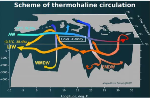
Figure 1.2: Schematic of Mediterranean Thermohaline Circulation. Modified by L.Houpert from
Tsimplis et al.(2006). AW=Atlantic Water, LIW=(Levantine Intermediate Water, WMDW=Western Mediterranean Deep Water, EMDW=Eastern Mediterranean Deep Water)
The heterogeneous nature of Mediterranean environment has always also fostered a multi-cultural community around its coastlines. Since the ancient times, Mediterranean Sea has been an important trading route and a cradle of many different civilizations, which flourised and interchanged. Today, it continues its significant contribution to global trade and economy, being also a hot spot for tourist activity. It is also a disputed space, with tensions between users and competition for resources. However, its densely-populated coastal cities (500 million inhabitants) of 23 modern states, are characterised by strong socioeconomic differences and face multiple environmental and social challenges. For example, in part related to climate conditions, they are exposed already to a deficit in freshwater resources, to an increase in heat stress and pollution that affect health systems, as well as to an intensification of extreme events (e.g droughts, flooding, heatwaves) that impact economies disproportionately (Navara and Tubiana,
2013). There seems to be a north-south gradient of increasing vulnerability to climate change similar to the north-south gradient in the area’s climate character. Relative to the northern countries, the southern regions demonstrate a lower adaptive capacity to changes in climate, due to reduced financial and technical resources, inadequate infrastructures and governance (Lionello et al., 2012). As a result of the great variety of socioeconomic activities, including tourism, recreation, fisheries, aquaculture, energy, cultural heritage uses, desalination, waste discharges, oil spills and maritime transport, the basin itself is under great human pressure. At the same time, it provides a wide range of ecosystem services upon which, the quality of life of neighboring communities and economic activities depend (Bleu, 2008). Therefore, a collective strategy in terms of management of marine resources, observation, monitoring and controls is required to increase resilience under climate change conditions.
The unique character of the Mediterranean Sea stands in that it is the largest and deepest enclosed sea on Earth (along with the Arctic Ocean) and a laboratory for the investigation of physical processes of global importance that operate within its small-scale subbasins. Apart from hosting a reduced version of the large-scale oceanic conveyor belt (Malanotte-Rizzoli et al.,2014), due to its semi-enclosed nature, it can be also used as a test bed for the evaluation of air-sea heat fluxes and the study of heat-budget (Bunker, 1982) and freshwater budget closures. Despite its small size, it is a biogeographical crossroad that responds quickly to atmosphere forcing and to anthropogenic influences. It represents only the 1.5% of the earth’s surface, yet, a plethora of risks encountered on global scale, for example, warming, drying, water cycle and biodiversity changes, land degradation, population growth, migration and conflicts, occur simultaneously and are aggravated here. Therefore, amongst the many pressures exerted on its fragile ecosystems, resources and communities, comprehension of the interplay between the large-scale forcing and the regional influences is of outmost importance. But a high-resolution is required to adequately represent the effect of the morphological diversity on its atmospheric and oceanic circulation. For this reason, the present doctoral thesis approaches the occurrence of extreme climate events in the Mediterranean Sea, using the latest available, high-resolution ensemble of dedicated, coupled Regional Climate System Models (RCSM) from the Med-CORDEX framework.
1.2
Modeling of the Mediterranean Climate System
For the assessment of climate changes in the Mediterranean domain between 1950-2100, different socio-economic scenarios and types of model projections have been used:1. General Circulation Models (GCMs), coupled Atmosphere-Ocean Global Climate Models (AOGCMs) and also Earth System Models (ESM), as part of coordinated Coupled Model Intercomparison Projects (CMIP). CMIP3-based results on the Mediterranean have been widely analyzed so far, whereas those by CMIP5 are still ongoing and outcomes of CMIP6 are to be expected in the coming years (Giorgi and Lionello, 2008;Lionello et al., 2012).
2. High-resolution, regional climate models (RCMs) dedicated to the Mediterranean region, by means of dynamically downscaled GCMs (AGCMs or AOGCMs). The RCMs then include: − 2a) Atmosphere-only models that are used to study the change of the atmosphere above the Mediterranean region, as part of international coordinated programs. For instance, in the following sections results from the multi-model ensembles of simulations developed within the PRUDENCE (Christensen and Christensen,2007) and ENSEMBLES (Van der Linden and Mitchell, 2009; Goodess et al., 2009) European projects will be often men-tioned. They comprise a number of GCMs and RCMs under the SRES-A2/B2 (PRU-DENCE, 50km) and SRES-A1B (ENSEMBLES, 25km) emission scenario. An extension to these is the EURO-CORDEX program (Jacob et al.,2013) that has a 12km horizontal resolution, run under RCP4.5 and RCP8.5 emission scenarios and cover a domain from Ireland to Red Sea.
− 2b) Forced regional ocean models used to assess changes for the sea (e.g. Somot et al.,
2006; Macias et al., 2018) and
− 2c) Fully-coupled, atmosphere-ocean regional climate system models (RCSM), where a high-resolution and high-frequency coupling is established between the various compo-nents of the regional climate system. For example, the European project CIRCE (e.g.
Dubois et al., 2012; Gualdi et al., 2013) has made a coordinated effort to analyze the performance of such models, which have only recently emerged (e.g. Somot et al., 2008;
Carillo et al.,2012), over the Mediterranean. More recently, however, the Med-CORDEX initiative (Ruti et al.,2016) has coordinated simulations using RCSMs under the RCP2.6, RCP4.5, RCP8.5 emission scenarios, with a ∼30-50 km resolution in the atmosphere (or even 25-50 Km AWI model, ENEA) and 9-25km varying resolution in the sea. For the purposes of this thesis, datasets from this ensemble of simulations will be used, which cur-rently constitutes the latest available, high-resolution Mediterranean-related multi-model ensembl.
3. Finally, statistical downscaling methods are also a common practice for the analysis of climate changes on atmosphere and land (e.g. Ozturk et al., 2015; Hertig and Jacobeit, 2008)