New method to detect convergence in simple multi-period market games with infinite large strategy spaces

(1)

HAL Id: halshs-01960900

https://halshs.archives-ouvertes.fr/halshs-01960900

Submitted on 19 Dec 2018

HAL is a multi-disciplinary open access

archive for the deposit and dissemination of sci-entific research documents, whether they are pub-lished or not. The documents may come from teaching and research institutions in France or abroad, or from public or private research centers.

L’archive ouverte pluridisciplinaire HAL, est destinée au dépôt et à la diffusion de documents scientifiques de niveau recherche, publiés ou non, émanant des établissements d’enseignement et de recherche français ou étrangers, des laboratoires publics ou privés.

New method to detect convergence in simple

multi-period market games with infinite large strategy

spaces

Jørgen Vitting Andersen, Philippe de Peretti

To cite this version:

Jørgen Vitting Andersen, Philippe de Peretti. New method to detect convergence in simple multi-period market games with infinite large strategy spaces. 2018. �halshs-01960900�

(2)

Documents de Travail du

Centre d’Economie de la Sorbonne

New method to detect convergence in simple multi-period market games with infinite large strategy spaces

Jørgen-Vitting ANDERSEN, Philippe De PERETTI

(3)

New method to detect convergence in simple multi-period market games

with infinite large strategy spaces.

Jørgen Vitting Andersen,, and Philippe de Peretti July 2018

_CNRS,_{Centre d’Economie de la Sorbonne, Université Paris 1 Pantheon-Sorbonne, Maison}

des Sciences Economiques,106-112 Boulevard de l’Hôpital, 75647 Paris Cedex 13, France.

We introduce a new methodology that enables the detection of onset of convergence towards Nash equilibria, in simple repeated-games with infinite large strategy spaces. The method works by constraining on a special and finite subset of strategies. We illustrate how the method can predict (in special time periods) with a high success rate the action of participants in a series of experiments.

Keywords: multi-period games; infinite strategy space; decoupling; bounded rationality; agent-based modeling

1 Introduction

Quite often, it can be difficult to obtain a proper behavioral prediction of people’s action in simple one-shot games, since it is obscured by non-equilibrium behaviors, which can persist even when the games are played repeatedly (Chong et al. 2016; Muller and Tan 2013). One question then, is how one can get a better understanding of the decision making in repeated games, and eventually dynamics hereof, before a proper equilibrium has set in? In Chong et al. (2016) a generalized cognitive hierarchy was introduced to capture the fact that subjects frequently do not play equilibrium in simple one-shot games, a behavioral trait which could be

(4)

because players are heterogeneous and have different levels of thinking ability. As will be explained below, different levels of thinking ability, and the impact it could have on the convergence to equilibrium is an important issue in both the experiments and modeling described in this article.

The situation we describe here becomes even more complex since we are considering the case when the strategy space available to people becomes infinite large. In situations like this it is unrealistic to think that people analyze an infinite possibility of strategies. Rather, it becomes more likely that people use heuristics (Crawford 2013), limiting the analyses to few simple and understandable cases. Then the question is, how one can try to catch such an analysis in a game theoretical framework?

Here we suggest one solution, which is to focus on a certain subset of strategies. The solution reminds of the study done by Ioannou and Romeo (2014), who introduced a methodology in order to facilitate operability of belief-learning models with repeated-game strategies. Since the set of possible strategies in repeated games is infinite (uncountable), expecting a player to fully explore such an infinite set is unrealistic. As noted in Ioannu and Romeo (2014), and in McKelvey and Palfrey (2001) there is also an inference problem even for games with only two players. In repeated games there is no unique way to tell an opponents strategy based just on the history, since several different strategies can lead to the same history. This point become even more relevant for the type of games we present in this study, where the history is created by several (N>2) players, making it impossible for a given player to know other playes precise strategies. Therefore, even though the history of play is publicly observed, a player will never be able to deduce the opponent’s precise strategy.

The solution of Ioannu and Romeo (2014) was to introduce repeated-game strategies implemented via a type of finite automaton, called a Moore machine, thereby limiting the

(5)

infinite repeated-game strategy space to a finite subset. In our study we will focus on another special subset of repeated-game strategies, called decoupled strategies, which have the special property of having their actions independent of the action history, conditioned on observing certain histories. As will be seen, this property allows us automatically to identify heuristic strategies, since at special moments the decoupled repeated–game strategies then effectively correspond to simple one-shot strategies. We would also like to point out the similarity to collective action games, see for example Anauati et al. (2016) who introduced a method of stability sets. They were able to capture the case where increases in the payoff of a successful collective action, led to upgrade in prior beliefs as to the expected share of cooperators.

2 Simple multi-period market games: theoretical framework

The introduction of the economist Brian Arthur of his famous El Farol bar game (Arthur 1994) set off a flurry of research in simple binary choice decision making models, with the decision of the type “go/stay”, “yes/no”, “buy/sell”, “right/left”, etc. In Arthur’s model a population of N=100 people want to go to the El Farol bar (an existing bar in Sante Fe) to listen to folk music. However, the El Farol is quite small, and people are only satisfied if they get seated on one of the 60 seats available. People have to make their decision at the same time, and so if everybody uses the same pure strategy, it will fail: suggesting “go” (assuming an empty bar) everybody will go and the bar be crowded, “stay” (assuming a crowded bar) instead will lead to an empty bar. Challet and Zhang (1997) extended the El Farol model in order to describe financial market behavior, now having the binary choice as a simple “buy/sell” decision. More precisely, in the minority game there is an odd number N of players who use different strategies in order to try to always be on the minority side. If a strategy 𝑆 , predicts the

(6)

majority will buy, then that strategy will recommend to sell, 𝑆 = −1. Otherwise, if predicting the majority will sell, the recommendation is to buy, 𝑆 = 1. The payoff of strategy i,

𝜋 (𝑠 ) = −𝑠 𝐴, 𝐴 = 𝑠

with A the order imbalance (i.e. the difference in buy and sell orders). As mentioned in Linde et al. (2014) already the one-shot minority game has quite a large number of Nash equilibria. This happens since any case where exactly (N-1)/2 players choose one side (and (N+1)/2

players the other side) constitutes a Nash equilibrium. The !

! ! Nash equilibria already

are quite a large number even for moderate values of N.

In the multi-round minority game, players then use strategies that consider the outcome of not only the last, but the past M market price directions (a positive order imbalance, A : the market goes up; A negative: the market goes down). Each player holds the same number of S strategies which are assigned randomly at the beginning of the game. A strategy in the multi-round issues a prediction (buy/sell) of the next market move for each of the possible 2 past

price histories. The total number of different strategies is therefore 2 . In the multi-round minority-game the players record the cumulative payoff for of each of their S strategies, and use the one which at a given time has the highest cumulative payoff. For an extensive review of the multi-round minority game see for example: (Cavagna et al. 1999; Challet et al. 2000a; Challet, et al. 2000b; Challet et al. 2001, Challet and Zhang,Y.C.,1998, Johnson et al 1999; Lamper et al. 2001.)

As mentioned in Andersen and Sornette (2003) one problem with the multi-round minority game describing simple market price dynamics, is that lack of speculative behavior where investors invest to gain a return. It should be noted that the minority dynamics prevents any

(7)

trend to develop, giving rise to a price dynamic which is mean reverting. In order to capture speculative behavior as seen in bubble/crash phases of financial markets, a modification of the payoff function was suggested in Andersen and Sornette (2003). Denoting the game, the $-game (to describe players that speculate), the modified payoff reads:

𝜋$ _{(𝑠 (𝑡)) = 𝑠 (𝑡 − 1)𝑅(𝑡)}

The payoff favors strategies which are able to predict the price movement over the following time step. Predicting at time t-1 an price increment over the following time step, the strategy i propose to enter a buy position at time t-1, 𝑠 (𝑡 − 1) = 1. If the prediction was successful (a failure) the payoff gained (lost) is the return of the market over that time step.

As mentioned the mere size of the strategy space for one-shot games, 2 , complicates considerably a proper understanding of simple market models like the minority game and the $-game, despite the simplicity of their payoff functions. It is therefore out of question to explore the full strategy space in order to gain insight on how people would react even in simple market games like this. We instead propose to concentrate on a certain subclass of strategies.

Let us call 𝑠 (𝑡 | ℎ⃗ (𝑡)) the action of strategy 𝑠 at time t, conditioned on observing a given

price history, ℎ⃗ (𝑡), at time t over the last M time steps. ℎ⃗ (𝑡) is a binary string of -1’s and +1’s describing the last M directions of price movements observed at time t. We now note that

some strategies will be independent of, ℎ⃗ (𝑡), over the next L time steps. That is, whatever price history over the next t + Q time steps, the strategy 𝑠 (𝑡 + 𝑄) will always issue the same prediction independent of the price history between t and t+Q. We call such strategies Q time steps decoupled (Andersen and Sornette, 2005). The most simple example of a strategy that is decoupled, is the strategy that always issues a buy (/sell) action, independent of the past price

(8)

the probability that any player will hold this specific strategy is very unlikely, with a probability

that goes as .

As will be seen in the following, it is advantageous to split the order balance in two, so that it can be written in terms of decoupled and coupled strategies:

𝐴(𝑡)⃗ = 𝐴(𝑡)⃗ + 𝐴(𝑡)⃗

We have added ℎ⃗ to emphasize that the order imbalance is conditioned on observing the

price history ℎ⃗ at time t.

The size of 𝐴(𝑡)⃗ /𝑁 then gives the percentage of decoupled strategies at time t,

and will be used as a predictor for the actions of the participants. In the extreme case where the condition:

|𝐴(𝑡)⃗ | > 𝑁/2

is fulfilled the prediction becomes certain, since the action at time t+2 of more than half the population takes the same sign (buy/sell) independent of what happens at time t+1. The larger

the size of 𝐴(𝑡)⃗ /𝑁, the better we should be able to predict the action at time t+2. This

fact will be used in the experiments where we try to predict the actions of the participants. For a discussion on the effect of group size N see also (Nosenzo et al., D. 2015)

3 Laboratory experiments

We performed a series of 10 experiments at the Laboratory of Experimental Economics in Paris (LEEP). The experiments ran over 60 periods. In each period, the students, received general economic news, and could decide whether to buy, or sell an asset, or simply do nothing. At the end of the 60 periods, the students were paid pro rata according to their performance (for more details about the way the experiments were set up, see “Appendix B”).

(9)

At the beginning of the experiment the students were told that the asset was, at this initial stage, properly priced according to rational expectations (Fama 1970; Muth 1961). This meant that only information regarding changes in the dividends on the asset or interest rates should have a direct influence on the price of the asset (for an interesting study with varying fundamental values, see e.g. Stockl et al. 2015). The information flow consisted of general news from past real records of Bloomberg news items. News was selected in such a way that the general trend over the 60 consecutive periods was neutral. Then, according to rational expectations, there should be no overall price movement of the asset at the end of the 60 time periods. The price was thus expected to oscillate around the fundamental value throughout the experiment.

4 Results

The Figs. 1-5 show the price history versus time for the ten experiments (E1-E10), as well as the decoupling parameter versus time obtained via Monte-Carlo (MC) simulations. Each figure represents the data and simulation from two experiments. The MC simulations “slaved” the price history from the experiments as input to the agents in the $G simulations. That is, instead of having the agents reacting to their own repeated-game actions, the agents in the simulations would instead use the actions (price history) of the participants. Each $G MC simulation was done with the number of agents fixed N=10 (number of participants in the experiments), but randomly generated initial strategies. The number of strategies used by the agents, S, and the memory, M, were also randomly generated S ϵ [1,Smax], M ϵ [1, Mmax] , with

Smax=10 and Mmax=6 reflecting the maximum values of memory and number of strategies

thought to be used by the participants in the experiments (we checked this assumption in interviews with the participants performed after the experiments). Simulations with larger

(10)

values of Smax and Mmax were performed showing the similar trends as presented in the

following. In total L=1000 MC simulation were performed for each experiment.

Figure 1 shows on the topmost plot the price evolution as a function of time for experiment E1. The second plot (from the top) shows the percentage of decoupled strategies (d+_{: decoupled}

strategies recommending buy, represented by a solid line; d-_{: decoupled strategies}

recommending sell, represented by a dashed line) used by the agents, as a function of time. The percentage for each time period t, is obtained as averaged over all MC samples.

Fig. 1. Two experiments E1, E2. First and third plot: price evolution of experiment E1 and E2 respectively. Second (E1) and fourth (E2) plots: solid line: d+_{, decoupled strategies}

recommending buy as a function of time. Dashed line: d-_{, decoupled strategies recommending}

(11)

We now use the difference Δ𝐷(𝑡) ≡ |𝑑 (𝑡)−𝑑 (t)| as a predictor of the action of the action of the participants in the next time step t+1. Table 1 shows ΔD for values larger than 0.2, the success rate in predicting the next price direction and the number of periods used in the calculation of the success rate. The experiment E1 corresponds to the simplest case of all the 10 experiments, since in this case the price dynamics created by the participants shows the formation of a clear financial bubble. This is captured by the split in decoupled strategies measured by 𝛥D leading to a 100% success rate. However, this is less trivial than it appears since as noted in Roszczynska et al. (2012) decoupling in strategies is a sufficient but not necessary condition for financial bubble formation. In other words: it is possible to have the onset of speculation without having a development of a split between 𝑑 (𝑡) and 𝑑 (t). For a clearer discussion on this point, see Roszczynska et al. (2012).

Table 1

ΔD , success rate, and corresponding number of events used in the calculation of the success rate, for experiment E1.

ΔD Success rate Number of events

0.2 1.0 46 0.22 1.0 45 0.24 1.0 44 0.26 1.0 44 0.28 1.0 43 0.3 1.0 41 0.32 - 0

(12)

Lower two plots of Fig. 1 show the price evolution and corresponding percentage of decoupled strategies for experiment E2. Again we see the tendency of the formation of speculative action, creating a financial bubble in prices, but a magnitude of 10 smaller than E1. Using 𝛥D as predictor we are again able to predict with high success rate the actions of the participants, see table 2.

Table 2

Fig. 2 shows the price evolution and corresponding percentage of decoupled strategies for experiments E3 and E4. In E3 an overall very weak trend is developing, whereas first part of E4 is trendless, followed by a weak upward trend and a finish by a small downward trend. Using 𝛥D as predictor we are again able to predict with a rather high success rate the actions of the participants, see table 3 and table 4. It should be noted the first half of E4 is trendless, still

0.2 0.70 27 0.22 0.68 25 0.24 0.73 22 0.26 0.69 16 0.28 0.62 13 0.3 0.64 11 0.32 0.67 6 0.34 0.75 4 0.36 - 0

(13)

as seen from figure 2 𝛥D is still large, and as can be seen from table 4, a reliable predictor even in this trendless case

sell as a function of time.

Table 3

ΔD , success rate, and corresponding number of events used in the calculation of the success rate, for experiment E3

0.2 0.57 23

0.22 0.67 15

0.24 0.67 3

(14)

Table 4

Table 5

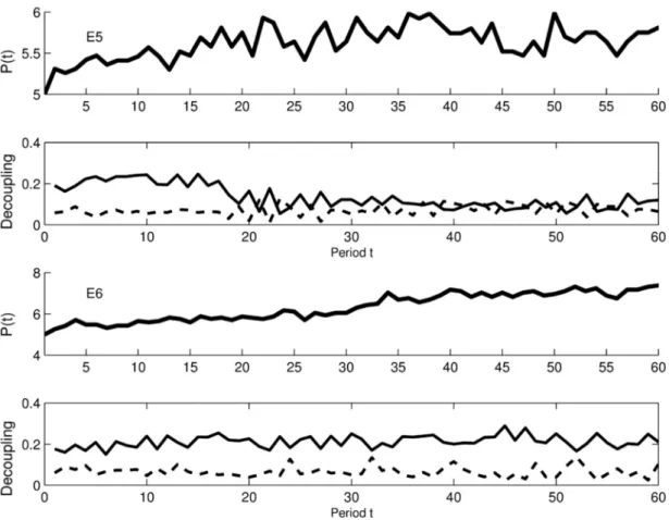
Fig. 3 shows the price evolution and corresponding percentage of decoupled strategies for experiments E5 and E6. Both experiments are more or less without a trend, with the price fluctuating around the fundamental value. A small split in 𝑑 (𝑡) and 𝑑 (t) is only seen for initial times in E5 whereas a split exists throughout E6. For E5 𝛥D never exceeds 0.2 and we can’t issue any prediction. For E6 𝛥D only exceeds the threshold value 0.2 in some few time

0.2 0.65 20 0.22 0.73 15 0.24 0.73 11 0.26 0.70 10 0.28 0.67 9 0.3 0.57 7 0.32 - 0

(15)

periods, but the few predictions that are issued appear to be slightly better than random or random, see table 6.

Table 6

(16)

Fig. 4 show the price evolution and corresponding percentage of decoupled strategies for experiments E7 and E8. Weak trends are developing in the price formation but not in the split of 𝑑 (𝑡) and 𝑑 (t). For these two experiments the days on which we can issue a prediction are to few to have any meaningful statistical significance.

0.2 0.63 8

0.22 0.50 4

0.24 0.50 2

(17)

Table 7

0.2 0.00 1

0.22 - 0

Table 8

Fig. 5 show the price evolution and corresponding percentage of decoupled strategies for experiments E9 and E10. There is no trend present in E9 whereas a very weak trend develops

0.2 1.00 1

(18)

in E10. A small number of splits 𝛥D are developing in E9, more in E10 but in both cases we are not able to make issue predictions.

(19)

Table 10

In order to test the stability of the Monte Carlo simulations we performed a series of bootstrap simulations. Fig. 6 show the bootstrap simulations performed on the data for the experiments E1, E2 and E3. Similar bootstrap simulations were performed for E4 and E5 with the same conclusions as noted in the following for E1, E2, and E3. The figures were obtained by simulating for each experiment, 100 Monte Carlo simulations and calculating d+_{and d}- _{. For each of the 100 Monte Carlo simulation, 100 more replica Monte Carlo}

simulations were then performed in order to be able to assign 90% and 10% confidence

0.2 - 0

(20)

levels. The results are presented in Fig. 6 where the solid lines represent a MC realisation of d+_{and d}-_{, whereas the dashed lines give the 90% and 10% confidence levels calculated}

using the 100 replica MC simulations. That is, in only 10% of the cases would the replica MC simulations find a value of d+_{below what was found by the MC simulation. Similarly}

in only 90% of the cases would the replica MC simulations find a value of d+_{not exceeding}

what was found by the MC simulation. As can be seen the levels of d+_{and d}-_{of the MC}

simulations are very stable, confirming the stability of our predictions obtained via the split in d+_{and d}-_.

(21)

Fig. 6. Bootstrap simulations performed on the data for the experiments E1, E2 and E3. The figures were obtained by simulating for each experiment, 100 Monte Carlo simulations and calculating d+_{and d}- _{. For each of the 100 Monte Carlo simulation, 100 more replica Monte}

Carlo simulations were then performed in order to be able to assign 90% and 10% confidence levels. Solid lines represent the result for a MC realization of d+ and d-, whereas the dashed

lines give the 90% and 10% confidence levels calculated using the 100 replica MC simulations. That is, in only 10% of the cases would the replica MC simulations find a value of d+_{(or d}-_{) below what was found by the MC simulation. Similarly in only 90% of the cases}

would the replica MC simulations find a value of d+_{(or d}-_{) not exceeding what was found}

by the MC simulation.

6 Conclusion

We have introduced a new methodology in order to describe the onset of convergence towards Nash equilibria, in simple repeated-games with infinite larges strategy spaces. The method works by constraining on a special and finite subset of strategies, which we called decoupled strategies. We performed 10 multi-period simple financial market experiments, and applied our methodology within the framework of a simple financial market game called the $-game. We have illustrated how the method was able to predict (in special time periods) with a high success rate the action of participants. We note that the methodology of

decoupled strategies is not limited to the $-game presented in this article, but can be applied in the context of any multi-period game.

(22)

Appendix A: The Nash equilibrium of the $-Game

The dynamics of the $-Game is driven by a nonlinear feedback mechanism because each agent used his/her best strategy (fundamental/technical analysis) at each time step. The sign of the

order imbalance, ∑ 𝑎∗ ℎ⃗(𝑡) , in turn determines the value of the last bit 𝑏(𝑡) at time 𝑡 for

the price movement history ℎ⃗(𝑡 + 1) = (𝑏(𝑡 − 𝑚 + 1), 𝑏(𝑡 − 𝑚), … , 𝑏(𝑡)). The * in 𝑎∗

denotes the best strategy (out of s possible) for agent i. The dynamics of the $-Game can then be expressed in terms of an equation that describes the dynamics of 𝑏(𝑡) as:

𝑏(𝑡 + 1) =  ∑ 𝑎∗ ℎ(𝑡) (1)

where  is a Heaviside function taking the value 1 whenever its argument is larger than 0 and otherwise 0, and ℎ(𝑡) = ∑ 𝑏(𝑡 − 𝑗 + 1)2 is now expressed as a scalar instead of a vector.

(23)

𝑎∗ ℎ(𝑡) = 𝑎 | ,…, ∑ ( ) ∑

∗ _{( )}

ℎ(𝑡) (2)

(2) expresses that the optimal strategy * of agent i is the strategy j which maximizes the $G payoff between time k=1 and k=t. Inserting (2) in expression (1) one obtains an expression that describes the $-Game in terms of just one single equation for 𝑏(𝑡) depending on the values

of the 5 base parameters variables (𝑚; 𝑠; 𝑁; ; 𝐷(𝑡)) and the random variables 𝑎 (i.e. their initial random assignments).

We would first like to point out an important difference compared to traditional game theory since in our game the agents have no direct information of the action of the other players. The only (indirect) information a given agent have of other agent’s action through the aggregate actions of the past, i.e. the past price behavior.

In the following we will consider the simple case where each agent only has s=2 strategies. Then considering only the relative payoff between strategy 𝑎 and 𝑎 simplify the equations considerable. Let the action of optimal strategy 𝑎∗_{be expressed in terms of the relative payoff,}

𝑞 , so as to formulate ∑ 𝑎∗ ℎ(𝑡) as follows

∑ 𝑎∗ ℎ(𝑡) = ∑  𝑞 ℎ(𝑡) 𝑎 ℎ(𝑡) + 1 −  𝑞 ℎ(𝑡) 𝑎 ℎ(𝑡) (3) Inserting (3) into (1) and take the derivative of 𝑏 in 𝑡 + 1

= 𝛿 ∑ 𝑎∗ ℎ(𝑡) ∑ 𝛿 𝑞 ℎ(𝑡) ( ) 𝑎 ℎ(𝑡) − 𝑎 ℎ(𝑡)

+ 𝑞 ℎ(𝑡) ( ) + 1 −  𝑞 ℎ(𝑡) ( ) (4)

Looking inside the bracket of the sum in (4), it follows that a change in ∑ 𝑎∗ ℎ(𝑡) can occur either because the optimal strategy changes and the two strategies for a given ℎ(𝑡),

(24)

𝑎 ℎ(𝑡) and 𝑎 ℎ(𝑡) , differ from each other (first term in the bracket). Furthermore, a change in ∑ 𝑎∗ ℎ(𝑡) can arise also because the optimal strategy changes its prediction for the given

ℎ(𝑡) (second and third terms in the bracket).

The change in time of the relative payoff 𝑞 is computed as follows

= 𝑎 ℎ(𝑡 − 2) ∑ 𝑎∗ ℎ(𝑡 − 1) − 𝑎 ℎ(𝑡 − 2) ∑ 𝑎∗ ℎ(𝑡 − 1) (5)

Using ℎ(𝑡) = ∑ 𝑏(𝑡 − 𝑗 + 1)2 and inserting (5) in (4) one obtains:

= 𝛿 ∑ 𝑎∗ ℎ(𝑡) ∑ 𝛿 𝑞 ℎ(𝑡) ∑ 𝑎∗ ℎ(𝑡 − 1)

a b(t − j − 1)2 − a ∑ b(t − j − 1)2 

𝑎 ∑ 𝑏(𝑡 − 𝑗 + 1)2 − 𝑎 ∑ 𝑏(𝑡 − 𝑗 + 1)2 

 𝑞 ℎ(𝑡) ∑ ( ) + 1 −  𝑞 ℎ(𝑡) ∑ ( ) (6)

If ∑ 𝑎∗ ℎ(𝑡 − 1) , ∑ 𝑎∗ ℎ(𝑡 − 2) , … , ∑ 𝑎∗ ℎ(𝑡 − 𝑚) have all the same sign, the right-hand-side of (6) becomes 0, thus proving that a constant bit 𝑏(𝑡), corresponding to either an exponential increase or decrease in price, is a Nash equilibrium.

Appendix B: Implementation of the experiments.

The number of participants in each experiment was fixed at 10. There was only one asset in our financial market which the participants could either buy or sell, short-selling being allowed. The initial price of the asset was fixed at 5 euros with an expectation of a 10 cent dividend payout at the end of the 60 time periods. Each of the 60 time periods lasted 15 seconds. In each

(25)

time period, the participants were presented brief statements of economic news and they could either buy or sell ONE asset or do nothing. The participants were told that the asset was correctly priced according to rational expectations (Muth, 1961), that is, the price of the asset was supposed to correctly reflect all future discounted cash flow accrued to the asset. The participants could, at zero interest rate, borrow money to buy shares, and short-selling was allowed. The general financial information was taken from real financial news items obtained on Bloomberg over a two week time period. Students were told the asset represented a portfolio of assets like an ETF or an index. They were all simultaneously presented with the same information, meant to reflect general financial news, e.g. good or bad US employment figures, commodity price changes, etc. The news items were the same in all experiments and were chosen without positive or negative bias.

At the end of each time period, the participants’ orders were gathered and a new market price calculated, based on the order imbalance (with sign and magnitude determining the direction and size of the price movement) (Holthausen et al. 1987). That is the price at time t is given by

𝑃(𝑡) = 𝑃(𝑡 − 1)𝑒 ( )/ where A(t) is the order imbalance at time t and b the liquidity of the market (in the experiments chosen as b≡ 10 ∗ 𝑁, representing a market crash/bubble of 10 percent when all N participants chose the same action) . This was then shown to the participants graphically on their computer screen. Throughout the experiment the participants had a continuous update of the number of shares held and their gains/losses.

At the end of each experiment, a pool of 200 euro was distributed pro rata among the participants who had a positive excess gain

(26)

Acknowledgments

This work was carried out in the context of the Laboratory of Excellence on Financial Regulation (Labex ReFi) supported by PRES heSam under the reference ANR-10-LABX-0095. It benefitted from French government support managed by the National Research Agency (ANR) as part of the project Investissements d’Avenir Paris Nouveaux Mondes (invesiments for the future, Paris-New Worlds) under the reference ANR-11-IDEX-0006-02.

References

Arthur, W. B., 1994. Inductive reasoning and bounded rationality. Amer. Econ. Rev. 84, 406-411.

Anauati, M. V., Feld, B., Galiani, S., Torrens, G., 2016. Collective action: experimental evidence. Games and Economic Behavior 99, 36-55.

Andersen, J. V., Sornette D. 2003. The $-game. The European Physical Journal B-Condensed Matter and Complex Systems 31(1): 141-145.

Andersen, J. V., Sornette D. 2005. A Mechanism for Pockets of Predictability in Complex Adaptive Systems. Europhysics Lett. 70, 697.

Cavagna,A.,Garrahan,J.P.,Giardina,I.,Sherrington,J.,1999.Thermal model for adaptive competition in a market.Phys.Rev.Lett.83,4429–4432.

(27)

Challet,D.,Marsili,M.,Zhang,Y.C.,2000a.Modelling market mechanism with minority game. Phys.A276,284–315.

Challet,D.,Marsilli,M.,Zecchina,R.,2000b.Statistical mechanics of systems with heterogeneous agents:Minoritygames.Phys.Rev.Lett.84,1824–1827.

Challet,D.,Marsili,M.,Zhang,Y.C.,2001.Stylized facts of financial markets and market crashes in minority games.Phys. A294, 514–524.

Challet,D.,Zhang,Y.C.,1998.On the minority game analytical and numerical studies. Phys. A256, 514–532.

Challet, D., Zhang, Y. C., 1997. Emergence of cooperation and organization in an evolutionary game. Physica A, 246(3) 407-418.

Chong, J.-K., Ho, T.-H., Camerer, C., 2016. A generalized cognitive hierarchy model of games. Games and Economic Behavior 99, 257-274.

Crawford, V. P., 2013. Boundedly Rational versus Optimization-Based Models of Strategic Thinking and Learning in Games. J. Econ. Lit. 51 (2), 512-527.

Fama, E. F., 1970. Efficient capital markets: a review of theory and empirical work. Journal of Finance 25, 383-417.

Holthausen R W, Leftwich R W, Mayers D., 1987. The effect of large block transactions on security prices: A cross-sectional analysis. Journal of Financial Economics, 19(2): 237-267.

Ifcher, J., Zarghamee, H. 2016. Pricing competition: a new laboratory measure of gender differences in the willingness to compete. Exp. Econ. 19: 642-662.

(28)

Ioannou, A. C., Romero, J., 2014. A generalized approach to belief learning in repeated games. Games and Economic Behavior 87, 178-203.

Johnson, N., F., Hart, M., Hui, P., M., 1999. Crowd effects and volatility in markets with competing agents. Physica A: Statistical Mechanics and its Applications, 269(1): 1-8.

Lamper, D., Howison, S., D., Johnson, N., F., 2001. Predictability of large future changes in a competitive evolving population. Physical Review Letters, 88(1): 017902.

Linde, J., Sonnemans, J., Tuinstra, J., 2014. Strategies and evolution in the minority game: a multi-round strategy experiment. Games and Economic Behavior 86, 77-95.

McKelvey, R., Palfrey, T. R., 2001. Playing in the dark: information, learning and coordination in repeated games. Mimeo.

Muller, W., Tan, F., 2013. Who acts more like a game theorist? Group and individual play in a sequential market game and the effect of the time horizon. Games and Economic Behavior 82: 658-674.

Muth, J., F. 1961. Rational expectations and the theory of price movements. Econometrica: Journal of the Econometric Society, 315-335.

Nosenzo, D., Quercia, S., Sefton, M., 2015. Cooperation in small groups : the effect of group size. Exp. Econ. 18: 4-14.

Roszczynska, M., Nowak, A., Kamieniarz, D., Solomon, S., Vitting Andersen, J., 2012. Short and Long Term Investor Synchronization Caused by Decoupling. PLoS ONE 7(12): e50700. doi:10.1371/journal.pone.0050700.

(29)

Stockl, T., Huber, J., Kirchler, M., 2015. Multi-period experimental asset markets with distinct fundamental value regimes. Exp. Econ. 18: 314-334.