HAL Id: tel-01656977
https://tel.archives-ouvertes.fr/tel-01656977
Submitted on 6 Dec 2017
HAL is a multi-disciplinary open access
archive for the deposit and dissemination of sci-entific research documents, whether they are pub-lished or not. The documents may come from teaching and research institutions in France or
L’archive ouverte pluridisciplinaire HAL, est destinée au dépôt et à la diffusion de documents scientifiques de niveau recherche, publiés ou non, émanant des établissements d’enseignement et de recherche français ou étrangers, des laboratoires
Electrical impedance tomography for void fraction
measurements of harsh two-phase flows : prototype
development and reconstruction techniques
Antoine Dupre
To cite this version:
Antoine Dupre. Electrical impedance tomography for void fraction measurements of harsh two-phase flows : prototype development and reconstruction techniques. Fluids mechanics [physics.class-ph]. Ecole Centrale Marseille, 2017. English. �NNT : 2017ECDM0005�. �tel-01656977�
Laboratoire d’Hydromécanique des cœurs et circuits, CEA Cadarache
THÈSE DE DOCTORAT
pour obtenir le grade de
DOCTEUR de l’ÉCOLE CENTRALE de MARSEILLE
Discipline : Instrumentation
ELECTRICAL IMPEDANCE TOMOGRAPHY
FOR VOID FRACTION MEASUREMENTS
OF HARSH TWO-PHASE FLOWS :
PROTOTYPE DEVELOPMENT
AND RECONSTRUCTION TECHNIQUES
.
par
DUPRE Antoine
Directeurs de thèse : BOURENNANE Salah, RICCIARDI Guillaume
Soutenue le 10 octobre 2017
devant le jury composé de :
H-M. Prasser
Professeur, ETH Zürich
Président du jury
B.M.E. Moldestad Professeure, University College of Southeast Norway Rapporteur
L. Rossi
Expert senior, CEA
Rapporteur
C. Bellis
Chargé de recherche, LMA CNRS
Examinateur
S. Mylvaganam
Professeur, University College of Southeast Norway
Examinateur
Abstract
Recent developments with data acquisition equipment have reduced the time required for image acquisition with electrical tomography, thereby bringing new opportunities for the study of fast-evolving two-phase flows. Amongst the numerous advantages of this imaging technique for multiphase flow related research are non-intrusiveness, high acquisition rates, low-cost and improved safety. A set of electrodes placed on the periphery of the pipe to be imaged is used to impose an electrical excitation and measure the system response. The distribution of phases inside the study volume distorts the electrical field in a characteristic manner. The objective of this thesis is to assess the potential of electrical impedance tomography at high acquisition rate. The first stage consists in developing a prototype sensor and assessing its performance with simplistic experiments. The system architecture employs voltage control of the excitation and therefore does not require the implementation of the conventional voltage-to-current converter module. A novel data collection method, the full scan strategy, is considered and provides correcting factors for the parasitic impedances in the system. The second stage is the image reconstruction from the measurement data. The approach considered in the thesis is to assume that flow regime identification techniques may provide valuable information on the phase distribution that can be injected in the inverse problem for imaging, thereby tackling the challenge of the non-linearity of the inverse problem. A method for horizontal air-water flow regime identification has been elaborated with an electrical capacitance tomography sensor and multiphase flow rig tried and tested. It is being adapted to the fast electrical impedance tomography prototype and upgraded to include vertical flow regimes. In parallel, an image reconstruction method has been developed based on the NOSER algorithm and a pseudo-2D postulate. The analysis of the reconstructed images for a set of benchmark experiments provide insights on the merits and deficiencies of the algorithm and of the prototype.
Key words: Electrical Impedance Tomography, Instrumentation, Two-phase Flows, Void Frac-tion
Résumé
Les récentes avancées technologiques des matériels d’acquisition de données ont permis de réduire le temps d’acquisition d’image en tomographie électrique, ce qui offre des oppor-tunités pour l’étude des écoulements diphasiques transitoires. Parmi les nombreux atouts de cette technique d’imagerie d’écoulements diphasiques, on peut citer son caractère non-intrusif, sa haute fréquence d’acquisition, son faible coût et sa fiabilité en termes de sûreté. Un ensemble d’électrodes placées sur le pourtour d’une conduite servent à transmettre une excitation électrique au milieu et à le sonder. Ainsi, la distribution des phases perturbe les champs électriques de manière charactéristique. L’objectif de cette thèse est d’évaluer le potentiel de la tomographie d’impédance électrique rapide. La première étape consiste au développement d’un prototype de capteur et à l’évaluation de sa performance par des essais simplifiés. L’architecture du système utilise un contrôle en potentiel du signal d’excitation et ne nécessite donc pas d’implémenter un module de conversion tension-courant. La seconde étape est la reconstruction de l’image à partir des données mesurées. L’approche qui a été considérée est de supposer une image approchée de la distribution des phases grâce à une identification du régime d’écoulement. Ainsi, le défi de résoudre un problème inverse for-tement non-linéaire est simplifié. Une méthode d’identification de régimes d’écoulements horizontaux eau-air a été élaborée avec un module de tomographie de capacitance électrique et une boucle d’essais hydrauliques déjà éprouvés. Cette technique est en cours d’adaptation au prototype de tomographie d’impédance électrique rapide et en amélioration grâce à l’in-clusion des régimes d’écoulements verticaux. En parrallèle, une méthode de reconstruction d’image a été développée, basée sur l’algorithme NOSER et un postulat pseudo-2D. L’analyse des images reconstruites à partir d’un set d’expériences de référence procure un aperçu des avantages et des défauts de la méthode et du prototype.
Mots clefs : Tomographie d’impédance électrique, Instrumentation, Ecoulements diphasiques, Taux de vide
Contents
Abstract (English/Français) i
List of figures / List of tables vii
1 Introduction 1
2 Prototype development 5
2.1 Overview of instrumentation for flow imaging . . . 5
2.1.1 Characteristic length and time scales of multiphase flows . . . 5
2.1.2 Main imaging techniques . . . 6
2.1.3 Electrical tomography techniques . . . 9
2.2 Overview of electrical impedance tomography . . . 12
2.2.1 Electromagnetism and forward problem . . . 12
2.2.2 Basic principle of data collection for EIT . . . 14
2.2.3 Towards high frame acquisition rates . . . 17
2.3 Hardware . . . 19
2.3.1 Test section . . . 19
2.3.2 Electrodes . . . 21
2.3.3 Signal generation and data acquisition . . . 24
2.3.4 Multiplexing . . . 25
2.4 Software and procedures . . . 28
2.4.1 Excitation signal . . . 28
2.4.2 Data collection strategy . . . 28
2.4.3 Digital signal processing . . . 29
2.4.4 Full procedure for fast EIT . . . 31
2.5 Performance assessment of ProME-T . . . 34
2.5.1 Noise and uncertainties in signals of ProME-T . . . 34
2.5.2 Repeatability of the EIT measurements . . . 36
2.5.3 Comparison with analytical and numerical solutions . . . 39
2.5.4 Acquisition of image sequence in fast mode . . . 41
2.6 Studies for fundamental understanding . . . 43
2.6.1 Signal settling time . . . 43
2.6.2 Electrode-electrolyte contact impedance . . . 44
3 Flow regime identification 53
3.1 Overview of flow regime identification . . . 53
3.1.1 Multiphase flow regimes . . . 53
3.1.2 Flow regime identification . . . 56
3.1.3 Research with electrical tomography . . . 57
3.2 Experimental setup and campaign . . . 59
3.2.1 Multiphase flow rig . . . 59
3.2.2 Instrumentation and ECT sensor . . . 61
3.2.3 Experiments . . . 62
3.3 Methodology for identification . . . 66
3.3.1 Data collection strategy of raw ECT signal . . . 66
3.3.2 Time series analysis for extracting dynamical features . . . 67
3.3.3 Eigenvalues analysis for extracting geometrical features . . . 68
3.4 Results . . . 71
3.4.1 Intermittent against continuous flows . . . 72
3.4.2 Annular against stratified flows . . . 72
3.4.3 Stratified smooth against wavy flows . . . 73
3.4.4 Plug against slug flows . . . 75
3.5 Extended methodology with simulations . . . 79
3.5.1 Numerical model and simulations . . . 79
3.5.2 Numerical validation of the criteria . . . 80
3.5.3 Estimation of phase fractions . . . 82
3.5.4 Adaptation to ProME-T EIT sensor . . . 83
4 Imaging 89 4.1 Overview of EIT image reconstruction . . . 89
4.1.1 Inverse problem . . . 90
4.1.2 Regularisation . . . 92
4.1.3 Image segmentation techniques . . . 93
4.2 Two-phase flow imaging method . . . 95
4.2.1 Forward problem with EIDORS solver . . . 95
4.2.2 3D inversion with NOSER algorithm . . . 98
4.2.3 Pseudo-2D image reconstruction . . . 101
4.3 Assessment of reconstruction images . . . 102
4.3.1 Benchmark experiments . . . 102
4.3.2 Cross-sectional average phase fraction . . . 103
4.3.3 Comparing adjacent, opposite and full scan strategies . . . 103
5 Conclusion 107
Bibliography 118
List of Figures
2.1 Bubble-size histogram in fast pressure transient experiment. Adapted from
Nakath et al. (2013) . . . 6
2.2 Flow measurement downstream of heating section, P=7.7 bar, G=300mkg2s,∆Tsub=35°C, q=7.64 kWm2. Adapted from Park (2013) . . . 6
2.3 Principle of the ROFLEX sensor. Adapted from Hampel et al. (2016) . . . 8
2.4 Typical echo sequence of MRI. Adapted from Joseph-Mathurin et al. (2010). . . 8
2.5 Wire-mesh sensor with orthogonal sets of transmitter and receiver wire-electrodes. Adapted from www.hzdr.de . . . 9
2.6 Most sensitive configurations to detect centre region of the model for neigh-bouring, opposite, cross and adaptive strategies. The black lines indicate the delimitation between zones of positive and negative sensitivity. Adapted from Kauppinen et al. (2006) . . . 16
2.7 Illustrations of adjacent (left), opposite (middle) and cross (right) data collection strategies . . . 16
2.8 Picture of the ProME-T prototype sensor . . . 20
2.9 CAD models of the test section in 3D configuration (left) and 2D configuration (right) . . . 20
2.10 Side view of the test section . . . 21
2.11 System for positioning of rods . . . 21
2.12 Simulation of total impedance for each of 120 excitation patterns, for different heights of the test section: Z=2 ,10, 200 mm . . . 22
2.13 Two illustrative cases of misplacement of electrodes . . . 23
2.14 Outline schematic of the ProME-T hardware - test section, multiplexing circuit and PXI card with the coupling leads to the test section with electrodes . . . 24
2.15 3D CAD model of the PCB board used in multiplexing . . . 26
2.16 Wiring details (schematic) of the PCB board used in multiplexing . . . 27
2.17 Wiring details (integration) of the PCB board used in multiplexing . . . 27
2.18 Flow diagram of frame acquisition procedure with ProME-T . . . 33
2.19 10 periods of low and high amplitude signals . . . 35
2.20 Spectra of high and low amplitude signals for a 1 Volt 5 kHz excitation . . . 36
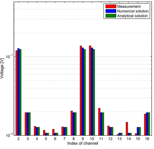
2.21 THD and SNR of signals on 16 measurement channels for 1 VAC 5 kHz excitation 37 2.22 Relative standard deviation of repeated identical measurements . . . 38 2.23 Comparison of analytical, numerical solutions and measurements on 16 channels 40
2.24 Comparison of numerical, analytical voltage profiles and experimental prediction 41
2.25 Image sequence at 667 fps of two gravitationally falling spheres: on the left, S1
with D1=22 mm,ρ1=5697 kg · m−3; on the right, S2with D2=25 mm ,ρ2=1144
kg · m−3 . . . 42
2.26 Illustration of settling signals in the four categories . . . 44
2.27 Analysis of the settling of signals in the four categories in terms of relative error 45 2.28 Electrical circuit model of the EIT system . . . 46
2.29 Modulus of impedance response of global impedance for various liquid conduc-tivities . . . 46
2.30 Phase of impedance response of global impedance for various liquid conductivities 47 2.31 Conductivity dependence of the indicators Rtand Xt(1Hz) . . . 48
2.32 Attenuation of capacitive effects with increasing excitation frequency . . . 49
2.33 Measured and calibrated impedance (3D) . . . 51
2.34 Measured and calibrated impedance (2D) . . . 51
3.1 Sketches of flow regimes for flow of air/water mixtures in a horizontal, 5.1cm diameter pipe. Adapted from Brennen (2005) . . . 54
3.2 Flow regime map for the horizontal flow of an air/water mixture in a 5.1 cm diameter pipe. Hatched regions are observed regime boundaries, lines are theoretical predictions. Adapted from Brennen (2005) . . . 55
3.3 Sketches of flow regimes for two-phase flow in a vertical pipe. Adapted from Brennen (2005) . . . 55
3.4 The vertical flow regime map of Hewitt and Roberts (1969) for flow in a 3.2 cm diameter tube, validated for both air/water flow at atmospheric pressure and steam/water flow at high pressure. Adapted from Brennen (2005) . . . 56
3.5 P&ID of the multiphase flow loop with ECT and GRM . . . 60
3.6 Photograph of the multiphase flow loop with ECT and GRM . . . 60
3.7 Test section with sensor placements, transparent section for high-speed cam-era based studies, multi-modal tomographic systems and differential pressure transmitters . . . 60
3.8 Twin plane ECT tomographic system – Arrays of 12 electrodes on the periphery of the pipe section with stratified flow in this schematic, Ca,bis the capacitance between electrodes a and b, with a,b = 1,2,...,12 . . . 62
3.9 Set of 115 experiments in the horizontal configuration, and the flow regimes as identified by experimental means (visual observation, GRM and high-speed camera recordings) . . . 63
3.10 Images of typical flow regimes (a) stratified smooth (b) low frequency waves (c) high frequency waves (d) annular (e) rear, bulk, and front of a plug (f ) rear, bulk, and front of a slug . . . 65
List of Figures
3.11 Representative arrays of 12 eigenvalues of the Cmeanmatrix for annular (in red),
stratified (in blue), intermittent flows (in green) and homogeneous flow (in black), obtained by averaging over the 115 measurements in the database. Error
bars indicate standard deviation in the data set . . . 70
3.12 Representative arrays of 12 eigenvalues of the CSDmatrix for annular (in red), stratified (in blue), intermittent flows (in green) and homogeneous flow (in black), obtained by averaging over the 115 measurements in the database. Error bars indicate standard deviation in the data set . . . 70
3.13 Flow diagram for regime identification method . . . 71
3.14 Parameter and indicator for Criterion I, on flow regime map . . . . 72
3.15 Parameter and indicator for Criterion II, on flow regime map . . . . 73
3.16 Spectra of normalised capacitance measurement ˆC12,12in 3 experiments: strati-fied smooth (blue), transitional (green) and stratistrati-fied wavy (red) flows. The 5 Hz cut-off frequency empirically set is indicated in black . . . 74
3.17 Illustrative example of slow instabilities . . . 75
3.18 Signal of theγ-ray densitometer for low frequency intermittent flow . . . 75
3.19 Parameter and indicator for Criterion III, on flow regime map . . . . 76
3.20 Spectra of normalised capacitance measurement ˆC3,5in 3 experiments: plug (blue), transitional (green) and slug (red) flows. The 10 Hz cut-off frequency empirically set is indicated in black . . . 77
3.21 Parameter and indicator for Criterion IV, on flow regime map . . . . 78
3.22 2D FEMM model of the ECT sensor, and mesh, illustrated for example of wavy flow 79 3.23 Array of 12 eigenvaluesλmean for stratified flows with various water fill levels . 82 3.24 Relationship between the cross-sectional averaged water fraction (WF) and the sum of eigenvaluesP12 i =1λ(i ), for stratified flows . . . 83
3.25 Sensitivity of the estimate for cross-sectional averaged water fraction (WF) to the sum of eigenvaluesP12 i =1λ(i ) . . . 84
3.26 Relationship between the cross-sectional averaged water fraction (WF) and the leading eigenvalueλ(12), for annular centred flows . . . 84
3.27 Pictures of the two extreme experiments in terms of WF: 48% (left) and 97% (right) 85 3.28 15 first elements of the array of eigenvaluesλ for annular flows with different water fraction . . . 86
3.29 Relationship between the cross-sectional averaged water fraction (WF) and the sum of the 15 eigenvaluesP15 i =1 ¯ ¯λ(i ) ¯ ¯, for annular centred flows . . . 86
3.30 CAD schematic of the new EIT sensor array and test section: 16 electrodes in yellow/orange, seals in red, test section made of PMMA in gray. Connections to the EIT modules are not shown. . . 87
4.1 Accuracy of simulations for meshes with various levels of refinement (varying maxszc yl) . . . 97
4.2 Accuracy of simulations for meshes with various levels of refinement (varying maxszel ec) . . . 97
4.3 L-curve method for assessing optimal regularisation parameter. Adapted from
Wei et al. (2015) . . . 99
4.4 Benchmark experiments result: real image on the left and reconstructed tomo-graphic image on the right . . . 103 4.5 Void fraction estimate from measurements, and real void fraction . . . 104 5.1 Schematic of EMFT sensor. Adapted from Leeungculsatien and Lucas (2013) . . 109
List of Tables
2.1 Comparison table of 3 fast EIT systems . . . 39
3.1 Summary table of the four criteria for eigenvalue based flow regime detection . 71
3.2 Numerical FEMM models, normalised capacitance matrices and arrays of
eigen-values, for each simulation of case study . . . 81
4.1 Linear back projection and other inverse reconstruction algorithms. Adapted
from Wei et al. (2015). . . 93
4.2 Set of images obtained with 5 inversion matrices (λr eg=0.00, 0.01, 0.05, 0.10 and
0.40). On the left, large cylinder ex-centred; on the right, large cylinder centred 100
Abbreviations
AT3NA Algorithme de Tomographie en 3D NOSER et Aplanissement (French)
CAD Computer aided design
CT Computed Tomography
DFT Discrete Fourier transform
ECT Electrical capacitance tomography
ERT Electrical resistance tomography
EIDORS Electrical Impedance Tomography and Diffuse Optical Tomography
Re-construction Software
EIT Electrical impedance tomography
FEM Finite element methods
FEMM Finite element method magnetics
fps frames per second
FRI Flow regime identification
GRM Gamma-ray meter
LBP Linear back projection
MRI Magnetic resonance imaging
NOSER Newton’s one-step error reconstruction
OZS Over-zero-switching scheme
PCA Principal component analysis
PCB Printed circuit board
PDF Probability distribution function
PMMA Polymethyl methacrylate
ProME-T Prototype pour Mesures Electriques par Tomographie (French)
PSD Power spectral density
SNR Signal to noise ratio
THD Total harmonic distorsion
UCSN University College of Southeast Norway
VCCS Voltage controlled current source
Notations and Symbols
A Some square matrix
Ae f f Effective area for current flow in 1D model
Al Surface of electrode-electrolyte contact area
Alin Linear contribution to the derivative of the Jacobian matrix
Anl Non-linear contribution to the derivative of the Jacobian matrix
~
B Magnetic induction field
C Capacitance matrix
Ca,b Capacitance between electrodes a and b
ˆ
Ca,b Normalized capacitance between electrodes a and b
Cx Drag coefficient
Cmean Capacitance matrix of mean of signals
CSD Capacitance matrix of standard deviation of signals
CLPxkHz Capacitance matrix of low-pass filtered signals
CHPxkHz Capacitance matrix of high-pass filtered signals
∆f Frequency resolution of DFT
∂Ω Periphery/boundary of the study volumeΩ
~
D Electrical displacement field
Di n Inner diameter of the ECT sensor
Dout Outer diameter of the ECT sensor
d L Misalignment of electrodes in 1D model
ηC Sensitivity of the ECT sensor array
² Electrical permittivity
²0 Vacuum permittivity
²R Relative permittivity of a medium
~E Electrical field
El Electrode number l
φ Objective function of least-square method
fac q Sampling frequency for acquisition
fEC T Frame acquisition rate of ECT sensor
fexc Frequency of excitation signal
γ Electrical complex conductivity G Conductance ˆ G Normalised conductance G Conductance matrix ~ H Magnetic H-field
H Axial separation of two rings of electrodes
HPxkHz High-pass filter operator with cut-off frequency of x kHz
I Electrical current
Il Electrical current at the electrode El
i Unit imaginary number
i R t R Sparse permutation matrix of the mesh
i R N Regularisation matrix
~J Electrical current field
J |∂Ω Neumann boundary condition
¯
Jm Lead field of current injection
¯
Jn Lead field of voltage measurement
Jac Jacobian matrix
λA Set of eigenvalues of A:
n
λ(i )
A, i = 1,2,...,12
o
λr eg Control parameter of the regularisation
L Separation between electrodes in 1D model
LPxkHz Low-pass filter operator with cut-off frequency of x kHz
LC Separation between sets of arrays of the ECT module
lC Length of electrodes of the ECT sensor
maxszc yl Maximum size of mesh elements (cylinder)
maxszel ec Maximum size of mesh elements (electrodes)
mean Mean operator
ν Outward unit normal to the boundary
Nf Number of frames per acquisition sequence
Nmesh Mesh cells in the forward model
Np Number of periods per excitation pattern
Ns Number of samples per excitation pattern
Nspp Number of samples per period of the excitation signal
~n Tangent to an infinitesimal surface
nC Number of electrodes of the ECT sensor
Ω Study volume
Ωk Volume of element k of the mesh
ω Angular frequency
Q Electrical charge on an electrode
List of Tables
Pr eg Penalty term of the regularisation
ρv Electrical charge density
R Electrical resistance
Rad d Additional resistance in 1D model
R M Inversion matrix in 3D
R M0 Inversion matrix in 2D
R M Sr c Root mean square of relative changes
Rs Sense resistor
Rt Resistive component of Z
σ Electrical conductivity
σb Surface of electrode b
SD Standard deviation operator
S Sensitivity coefficient
S(Ei, Ej) Excitation pattern with Eias source and Ejas drain
Si Set of excitation patterns, i=1,2,...,120
τ Transit time of the dispersed phase between two rings of electrodes
T Threshold of a criterion
V Electrical (scalar) potential
ˆ
Vi Normalized voltage measurement on channel n°i
V |∂Ω Dirichlet boundary condition
Vi Voltage measured on channel n°i
Vmea Set of voltages in the measurement frame
Vr e f Set of voltages in the reference frame
Vsi m Simulated set of voltages
~vA Set of eigenvectors of A
vt er m Terminal velocity
vz Axial velocity of the dispersed phase
wC Width of electrodes of the ECT sensor
Xt Reactive component of Z
x Some point in the study volumeΩ
xDF T DFT of sampled signal xsi g
xsi g Sampled signal
Z Total impedance of the EIT system
Zbul k Bulk impedance of the medium
Zd r ai n Drain electrode-specific impedance
ZSi Total impedance for the i
th excitation pattern
1
Introduction
Background
Tomography refers to the imaging of a volume. The word is derived from ancient Greek:
τoµ´η, tomi for a volume or a section, and γρ ´αϕω, grafo for writing. The underlying feature
of tomography is the study of an excitation generated outside the boundary and interacting with the medium inside the volume. The science has emerged with the use of X-ray radiation
as an extension of radiography. The discovery of X-rays by R¨ontgen in 1895 rapidly led to
the birth of radiology as a medical imaging technique. Typically, X-rays are generated by the Bremsstrahlung effect. A voltage being set between an anode and cathode in a vacuum tube, stream of electrons are directed toward the anode where the sudden deceleration by collision generates electromagnetic radiation at wave-length corresponding to X-rays. The radiation propagates within the study volume or human body to a detector. In the early stage of radiology, a photographic film would be used to develop an image. Yet, each pixel would contain the condensed information on the material properties integrated along the transmission path of the rays, i.e. a projection. In other words, shadow effects were (and still are) challenging for the interpretation of radiographies. The earlier proposition of tomography could be traced back to Italian radiologist Alessandro Vallebona (Kevles, 1997) and his proposal of focal plane tomography. Moving synchronously and in opposite directions both the source and the detector, the optical focus is kept at the focal plane while the contribution of out-of-focus zones is effectively cancelled out. The mathematical foundations of the computed tomography have been formulated by Austrian mathematician Johann Radon (Radon, 1986). The contribution of each pixel in a cross-sectional image is obtained by the Radon transform of a set of line integrals obtained with multiple projections. Considerations of image acquisition speed led to new generations of radiation-based tomography, with multiple sensors and/or detectors. The principle of tomography has been applied in various research fields: geophysics, material sciences, archaeology, etc. Different types of excitations have been used: radiation
(X-rays,γ-rays), pressure waves (sounds and ultrasounds), etc. Amongst others, low-frequency
electrical currents brings interesting perspectives for flow monitoring research and industrial applications.
Multiphase flows are frequently encountered in many research fields and industrial applica-tions. Understanding their dynamical evolution is important to assess heat transfer, fluid-structure interactions or reaction kinetics. A single phase flow is characterised by the density and velocity fields. The conservation of mass, momentum and energy provides the equations describing the dynamics. Viscous effects can play an important role. Single phase flows are frequently sorted into the laminar, intermediate and turbulent categories according to their Reynolds number. The comprehension of multiphase flows is more complex since interaction between phases needs to be taken into account. The topology of multiphase flows are relatively few and dependent on the prevailing rheological mechanisms. The basic approach of con-sidering homogeneously mixed phases frequently fails and tomographic measurements are essential in order to provide reliability in identifying flow regimes and their characterisations. Imaging a multiphase flow consists in measuring the distribution of phases and provides information on the phase indicator functions. If either the spatial or temporal resolution cannot match the characteristic time and length scales of the flow under investigation, the locally space-averaged or time-averaged phase fraction takes a value in the range between 0 and 1. For gas-liquid two phase flows, this is often referred to as void fraction.
In imaging of multiphase flows, a high frame rate and fine spatial resolution are desirable. Instrumentation techniques can be categorised according to their intrusiveness. Intrusive sensors such as optical probes or wire-mesh do not necessarily perturb the flow significantly. However, their integration in high pressure high temperature flow facilities raises complex challenges. In some industrial applications, compatibility with harsh flows is required. Electri-cal Impedance Tomography (EIT) is an instrumentation technique for non-intrusive imaging of the distribution of the electrical properties of a medium (conductivity and/or permittivity). Under assumptions appropriate for specific experiments, this result can be transposed into images of phase distribution, temperature profiles, defects density, etc. Electrical tomography techniques feature non-intrusiveness, high acquisition rates, and low cost. However, low frequency electrical currents are so-called soft fields, which generates complexity in the image reconstruction. Active research in medical and geological applications has provided interest-ing findinterest-ings regardinterest-ing the spatial resolution of electrical tomography images. The research on high frame rate measurements with electrical tomography is far more recent.
Thesis organisation
The main objective of this thesis is to assess the capability of electrical tomography for the high acquisition rate measurements of void fraction in high pressure high temperature two-phase flow experiments. The long-term target is to integrate this instrumentation in experiments at conditions representative of the primary and secondary circuits of nuclear pressurised water reactors of generations II and III. This introductory chapter explains the motivation for the work. An overview of the recent knowledge of electrical tomography has helped selecting Electrical Impedance Tomography for the research. The main challenge foreseen at the start of the Ph.D. was the non-linearity of the inverse problem of electrical tomography for high
contrast conductivity imaging. However, a solution to mitigate this issue was postulated: consecutive images in the sequence are relatively similar for high frame rate measurements so the previous image may be used as the a priori solution of the linearised inverse problem. The plan of the thesis has been oriented as follows. This first introductory chapter described the background of tomographic imaging of multiphase flows. The second chapter describes the development of a prototype fast EIT sensor. The electrical potential of the excitation signal is controlled, providing interesting feature to the prototype sensor. In particular, the implementation of a module for voltage-to-current conversion is not necessary. A novel data collection method is proposed: the full scan strategy with 120 excitation patterns for a 16 electrodes sensor. The design of the system enables frame acquisition rates up to 833 frames per seconds with the full scan strategy. An overview of research and reports on existing EIT systems gives the motivation for the main technological features of the prototype. The hard-ware, software and procedures of the prototype are presented. Studies have been performed to assess the performance of the system and will also be reported. The third chapter explains the approach of flow regime identification using the raw measurement data. The principle is to recognise the flow regime and obtain associated parameters (e.g. cross-sectional void fraction) with a set of unprocessed data. The results might be considered as an approximate model of the flow, or as a priori information for the inverse problem. A brief introduction on the concept of flow regimes and an overview of state-of-the-art flow regime identification methods are presented. The work has been performed in the framework of a collaboration with Professor Saba Mylvaganam of University College of South-East Norway, before the prototype had been finalised. Details on the set-up of the flow facility and the Electrical Capacitance Tomography (ECT) sensor used in this study are given. The experimental campaign is described and the cri-teria developed for the flow regime recognition are shown. The flow regime provides an input for the image reconstruction method suggested in this thesis. The fourth chapter concerns the development of an image reconstruction algorithm. An extensive overview of the state-of-the-art in this field is presented. A method for image reconstruction has been developed within the framework of this thesis. It is based on the NOSER algorithm and a pseudo-2D postulate. The different steps of the method are presented and explained. Experiments has been performed in order to build a set of benchmark data presented in Appendix. The performance of image reconstruction is tested and comparison are made to highlight the role of some parameters. A concluding chapter summarises the findings and suggests some strategies for continuation of the project.
Notes and publications
An effort was put on the communication of the results of the Ph.D. research towards the
scientific research community. At the 7t hInternational Symposium on Process Tomography
(Dresden, Germany, September 2015), preliminary results on piecewise-constant binary recon-struction of tomogram have been presented (Dupré et al., 2015). At the Specialists Workshop on Advanced Instrumentation and Measurement Techniques for Nuclear Reactor Thermal
Hydraulics (Livorno, Italy, June 2016), the features of the ProME-T prototype sensor and per-formance assessment studies have been reported (Dupré et al., 2016a). The content has also
been published in the IEEE Sensors Journal (Dupré et al., 2017). At the 8t hWorld Congress on
Industrial Process Tomography (Foz do Iguacu, Brazil, September 2016), the results of the flow regime identification study with the ECT sensor has been shown (Dupré et al., 2016b). The content has also been accepted by the IEEE Sensors Journal and will be published in a special issue on Process Tomography (Dupre et al., 2017).
2
Prototype development
The basic principle of data collection in Electrical Impedance Tomography (EIT) consists in sequentially generating electrical excitations at selected pairs of electrodes and measuring the resulting voltage on all other electrodes distributed around the study volume. This chapter concerns the development of the prototype fast EIT system. The problem of processing the data to extract information or an image is left for the subsequent Chapters 3 and 4.
2.1 Overview of instrumentation for flow imaging
For a correct understanding of two-phase flows, it is important to develop instrumentation capable of measuring locally the void fraction and the phase velocities with adequate spatial and temporal resolutions. Development for instrumentation for high pressure high temper-ature flows is challenging. The next Section 2.1.2 gives a brief description of many imaging modalities that have been widely used in multiphase flow studies. Electrical tomography techniques are explained in more details in the subsequent Section 2.1.3.
2.1.1 Characteristic length and time scales of multiphase flows
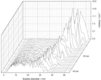
The spatial and temporal resolution of an instrument for imaging a multiphase flow ideally should match its characteristic length and time scales. This is specific to a given application and experimental set-up. With increasing pressure, the size of the bubbles in gas-liquid dispersed flows shrinks and their velocity increases. The study of Nakath et al. (2013) illustrates the effect of pressure on the bubble-size distribution during fast pressure transient in nuclear pressurised water reactors in accidental scenarios. The results of this study are shown in Figure 2.1. Small bubbles of diameter in the order of the millimetre are encountered in this study of multiphase flows.
Amongst many other examples, the heat transfer downstream of the heating section is an important phenomenon to be understood in many energy systems. The experimental data for understanding heat transfer not only consists of the cross-sectional average phase fraction,
Figure 2.1: Bubble-size histogram in fast pressure transient experiment. Adapted from Nakath et al. (2013)
but also of the topology of the flow. Sub-cooled flow boiling for advanced compact heat exchangers has been analysed with a high-speed camera in Park (2013). Number distribution of bubble diameter and size-velocity diagram are shown in Figure 2.2. If the characteristic time scale of a bubble flow is taken as the minimum time for bubbles to move by their diameter, in Park’s study it would be in the order of the millisecond (e.g. 0.002 s for the 0.5 mm diameter
bubble group with velocity 250 mm · s−1).
Number distribution of bubble diameter Size-velocity diagram
Figure 2.2: Flow measurement downstream of heating section, P=7.7 bar, G=300 mkg2s,
∆Tsub=35°C, q=7.64 kWm2. Adapted from Park (2013)
2.1.2 Main imaging techniques
X-ray tomography is a widespread imaging technique that has emerged from medical applica-tions. Electrons are accelerated from an anode to a cathode where the Bremsstrahlung effect
2.1. Overview of instrumentation for flow imaging
corresponding to the deceleration of electrical charges is responsible for the local emission of
X-ray. Theγ-ray tomography is a close relative that uses a radioactive material as a source of
γ-rays. The attenuation of a collimated beam along a straight line (called ray sums) gives an
information on the material composition along the path of the projection. A set of projections needs to be recorded in order to obtain information throughout the study volume. In the image reconstruction, also referred to as computed tomography (CT), mathematical opera-tions such as the Radon transform are performed (Plaskowski et al., 1995). For a complete scan of all projections, both the source and the detectors had to be moved in systems of the first generation. In subsequent generations, detector panels and then source arrays were developed in order to speed up the acquisition. In ultra-fast X-ray tomography, an electron beam is directed to a metallic target thereby enabling fast scanning of all angular positions without any mechanical parts moving (see Figure 2.3). This state-of-the-art technique features a high spatial and temporal resolution in the order of 1 mm and 10000 frames per second (fps) respectively (Banowski et al., 2015; Hampel et al., 2016). While the imaging capabilities of
X-ray andγ-ray tomography are outstanding, the safety measures associated with the use of
ionising radiation and the operational costs are a burden. The reduction of the acquisition time comes at the expense of degraded spatial resolution, especially in the former generations of instruments. Finally, the high attenuation of the signal in metals associated with the dose limits are problematic for the use in metallic pipes and other complex geometries.
Magnetic Resonance Imaging (MRI) also originates from medical applications (Mansfield, 2003). In presence of a magnetic field, the magnetic moments of nucleus or electrons in the matter react in an identifiable manner to a sequence of radio-frequency pulses (see Figure 2.4). The study volume is scanned by controlling gradients of the magnetic field, thereby obtaining an image. The spatial resolution can be quite accurate when phases have similar magnetic susceptibility ensuring homogeneity of the applied magnetic field (≈1 mm resolution). The temporal resolution is dependent on the ratio between the field of view and the resolution limit. It ranges in the order of 100 ms for a 256 × 256 pixel image and 10 ms for a 64 × 64 pixel image (Mansfield, 2003). This imaging technique has been applied for analysis of oil-water flow (Lakshmana et al., 2015), and the proposed echo sequence took about 100 ms.
Ultrasound tomography scans a study domain via a pressure wave applied at multiple bound-ary source locations. The transmitted and reflected waves are characterised by an attenuation coefficient (frequency dependent) and a propagation time. The former is closely dependent on the void fraction in the sensitive volume while the latter yields valuable information on the topology of interfaces (Plaskowski et al., 1995). This measurement technique shows limita-tions for high void fraction content since a continuous incompressible phase is needed for the transmission of pressure wave. Furthermore, the propagation velocity in the domain puts a limit on the acquisition time of an image (in the order of 10-100 ms in the study of Opielinski and Gudra (2006)). Yet, the technique has been proven to be very successful for the precise measurements of micro-bubbles and ultra-low void fractions (Cavaro et al., 2013).
Figure 2.3: Principle of the ROFLEX sensor. Adapted from Hampel et al. (2016)
Figure 2.4: Typical echo sequence of MRI. Adapted from Joseph-Mathurin et al. (2010).
et al., 1998). A mesh of wire-electrodes covers the inner cross-section of a pipe. The sensor measures the capacitance between transmitter and receiver wire-electrodes, which can be related to the local volume-averaged void fraction within the sensitive volume around the
2.1. Overview of instrumentation for flow imaging
crossing of the two perpendicular wire-electrodes (see Figure 2.5). In order to capture an image, transmitters are activated sequentially using a multiplexing unit and the signals at the receivers are sampled simultaneously with parallel sample-and-hold circuits. The technique features a very high acquisition rate up to 10 kHz and an excellent resolution limit of the order of 3 mm (Banowski et al., 2015). Despite its intrusiveness, the design of the wire-mesh sensor has been improved and it has been used in the studies of harsh flows (Pietruske and Prasser, 2007). Also, interesting studies present the analytical method to determine interfacial area density from the gradient of void fraction which gives valuable insight on the heat transfer processes (Prasser et al., 2015). Yet, the integration in high pressure high temperature environments remains very challenging. Thicker wires need to be used to ensure sufficient robustness, so the intrusiveness of the sensor will be more pronounced. Higher vibrations of the wires mean the distance between the transmitters and the receivers needs to be increased, thereby requiring larger mesh and degraded spatial resolution.
Figure 2.5: Wire-mesh sensor with orthogonal sets of transmitter and receiver wire-electrodes. Adapted from www.hzdr.de
2.1.3 Electrical tomography techniques
The key advantages of electrical tomography techniques are non-intrusiveness, high acqui-sition rates and cheap costs. An excellent overview of the instrumentation used in process tomography is given in Plaskowski et al. (1995), with a particular emphasis on electrical tomog-raphy. The principal categories of electrical tomography techniques are Electrical Impedance Tomography, Electrical Capacitance Tomography and Electromagnetic Tomography. As in any tomographic modality, the distribution of a parameter within a study volume is to be determined from a set of projections, i.e. measurements of the system response for a scan of excitations generated from the boundary of the test section. The Maxwell equations describe the electromagnetic behaviour in a given medium with know electrical properties. The ma-jor difference with radiation-based tomography techniques is that low-frequency electrical
currents are soft-fields: the sensitivity of a measurement is dependent on the distribution of materials in the study volume. Therefore, the concept of transmission paths or spatial resolution does not hold for soft-field tomography techniques though it can be approximated for a reference medium, as in Seagar and Bates (1985). The set of Maxwell equations and boundary conditions for all excitations used is referred to as the direct problem. Reciprocally, the distribution of electrical properties can be retrieved from a set of boundary excitations and measurements using reconstruction methods to solve the so-called Calderon’s inverse problem (Calderón, 2006). In multiphase flow imaging, the distribution of phase (more specif-ically the local pixel-averaged void fraction) can be retrieved from the image of electrical properties via the Maxwell-Hewitt relation that assumes homogeneous mixing locally (George et al., 2000).
Electrical Impedance Tomography uses low frequency current excitations to probe the electri-cal conductivity and permittivity profiles of materials within a study volume. Electrodes are distributed around the test section. For each excitation pattern, a pair of electrodes is selected and connected to the current source and sink. The response of the system is measured either as the absolute voltages of electrodes or as the differential voltages between neighbouring electrodes. Electrodes are directly in contact with the conductive continuous phase within the study volume in order to ensure that the electrical conduction of the current is the prevailing electromagnetic phenomenon. In studies considering water as the continuous phase, it is frequent to consider the addition of electrolytes and select excitation frequencies in the range 10-100 kHz (George et al., 2000; Wang, 2005).
Electrical Capacitance Tomography uses high frequency voltage excitation to probe the elec-trical permittivity of materials within a study volume. Electrodes are mounted on the outer surface of the pipe, not in direct electrical conductive contact with the study volume. ECT systems are non-intrusive and non-invasive. A high amplitude high frequency electrical poten-tial is set at one electrode while the resulting charges on the other electrodes (kept at ground potential) are measured and capacitance between each pair of electrodes computed. The procedure is repeated until all electrodes have acted as source once (Huang et al., 1988). Since the ECT signals are extremely weak, a considerable effort on pre-amplification and signal conditioning is crucial. Furthermore, a reasonable sensitivity can only be achieved with large surface electrodes (Ahmed and Ismail, 2008), which puts a limit on the spatial resolutions achievable with this modality. The prevalence of the displacement current means that there are no requirement on the conductivity of the materials to be imaged. As a result, this tech-nique is appealing for studies on chemical bed reactors and gas-particle flows. Electrodes being mounted on the outer diameter of the pipe/vessel, a dielectric material needs to be selected. Therefore, ECT is not suitable for high pressure high temperature applications that requires a metallic pipe to withstand the mechanical and thermal loads.
Electromagnetic Tomography stimulates the study volume using a set of magnetic fields generated by coils distributed around the test section. The induce voltages at the non-activated coils are recorded, and they are impacted by the generation of eddy currents within the
2.1. Overview of instrumentation for flow imaging
sensitive volume. As a result, the signal is related to the electrical conductivity and/or the magnetic permeability of the materials (Terzija et al., 2011).
The main instrumentation techniques for imaging of multiphase flows present limitations at high pressure and temperature. In harsh flow imaging applications, the pipes or the vessel are inevitably made of metal which prevents the use of non-invasive arrays of ECT electrodes. The spatial resolution of EIT is better and its implementation easier.
2.2 Overview of electrical impedance tomography
This section is an introduction to the the electromagnetic theory and basic principles of data collection for EIT. An overview of reported fast EIT sensors, recent trends and findings is proposed so the reader will have a clear idea of the state-of-the-art for this active research field.
2.2.1 Electromagnetism and forward problem Electromagnetism
Electrodynamics is the branch of physics relating electrical charges and currents. Maxwell equations describe electromagnetic phenomena up to the length scale and field strengths where quantum electrodynamics applies:
~∇· ~D = ρv, (2.1) ~∇· ~B = 0, (2.2) ~∇×~E = − ∂ ∂tB ,~ (2.3) ~∇× ~H =~J+ ∂ ∂tD.~ (2.4)
with ~B the magnetic induction field, ~H the magnetic H-field, ~J the electrical current, ~D the
electrical displacement, ~E the electrical field andρvthe electrical charge density.
The constitutive equations (i.e. its electrical properties of materials) relate the electrical
current ~J and displacement ~D to the electrical field ~E :
~J= σ~E, (2.5)
~
D = ²~E , (2.6)
whereσ and ² are the electrical conductivity and permittivity of a given material.
Considering the divergence of (2.4) and using the constitutive equations (2.5) and (2.6) results in: ~∇·µσ~E + ²∂ ∂t~E ¶ = ~∇ · (~∇ × ~H ) = 0. (2.7)
Electrical tomography techniques (EIT and ECT) are applications in which fluctuating mag-netic fields play a negligible role in comparison with electrical current and/or displacement.
As a result, one can notice in Equation (2.3) that the electrical field ~E is conservative since
2.2. Overview of electrical impedance tomography
Equation (2.7) can be recast in the frequency domain with a phasor transformation: ∂t∂~E = iω~E,
with i the unit imaginary number andω the angular frequency and results in the following
formulation for the forward problem within the study volumeΩ:
~∇·¡γ~∇V ¢ = 0, x ∈ Ω, (2.8)
withγ = σ+iω² the electrical complex conductivity. For the sake of clarity in equations, we
use shorthand notation for V ,γ, σ and ² though, as scalar fields, they are functions of x ∈ Ω.
Bates (1984) gives a generalised theory of full-wave problems. Low-frequency electrical current belong to the simplified category of conservative fields (like stationary magnetic fields and streamlined fluid flow) (Seagar and Bates, 1985).
Tomography
In electrical tomography, electrical currents J are sourced or drained onto the periphery of the
study volume∂Ω. The continuum model of electrodes (Cheney et al., 1990) gives the following
boundary condition:
−σ∂V
∂ν = J, x ∈ ∂Ω, (2.9)
withν the outward unit normal to the boundary.
There are other approaches to model the electrodes with various degrees of approximation of
the real physics. In the gap model, a current Ilis set at each electrode (El, l=1,2...,L) and the
current density is assumed to be constant throughout the electrode-electrolyte contact area Al,
as in equation (2.10) (Cheney et al., 1990). The shunt model adds the influence of the highly conducting electrode contact area on the electromagnetic behaviour near the electrodes. The complete electrode model is the compilation of the continuum model with the description of the shunt effect and of the contact impedance phenomenon (Hanke et al., 2011).
σ∂V ∂ν = Il Al for x ∈ El, l = 1,2,...,L 0 for x ∉ L S i =1 El . (2.10)
The materials within the study volume do not store electrical charges, as a result all currents flowing into the test section are necessarily flowing out:
Z
x∈∂ΩJ d x = 0.
The reference electrical potential may be chosen arbitrarily as: Z
x∈∂ΩV d x = 0. (2.12)
The set of Equations (2.8), (2.9), (2.11) and (2.12) replicated for every excitation patterns considered in the data collection strategy is frequently referred to as forward or direct problem in the literature (Tanushev and Vese, 2007).
It can be solved numerically with the methods of finite elements (George et al., 2000), finite volumes (Tanushev and Vese, 2007) or boundary elements (Peytraud, 1995). Approximations or simplifications can be used to reduce the computational cost, in particular in simple geometric setups such as cylindrical study volumes (Kotre, 1988; Nissinen et al., 2013). A few special cases have known analytical solutions (Pidcock et al., 1995; Torczynski et al., 1996; Seagar and Bates, 1985).
An open-source free software has been developed within the framework of the Electrical Impedance Tomography and Diffuse Optical Tomography Reconstruction Software (EIDORS) project (Polydorides, 2002). A flexible set of Matlab routines is provided for solving the forward and inverse problems of electrical tomography. The meshing can be provided by Netgen. Many examples are available. The software is very popular within the electrical tomography community and has been used in this thesis.
2.2.2 Basic principle of data collection for EIT
In practice, a finite set of electrodes (typically 16 or 32 in EIT, 8 or 12 in ECT) is available for the generation and the acquisition of electrical signals. Generally, in research or industrial applications, a simplistic 2D or 3D cylindrical study volume is being considered and the electrodes are arranged as a ring (regularly spaced in one cross-sectional plane). In typical procedures for EIT, a current is generated with a Voltage Controlled Current Source (VCCS) and the source and drain ports are connected to the current injection electrodes. Multiplexers (MUXs) "usually implemented using solid state switches" control the selection of the current injection electrodes (York, 2001). In parallel, the resulting voltage are measured synchronously on all available electrodes. Some set-ups consider the measurement of differential voltages between neighbouring electrodes, while others measure the absolute electrode potentials with respect to a common ground reference. The former is an efficient method to suppress common-mode parasitic noises, while the latter can suffer from potential biases in the com-mon ground. In this thesis, the set of measurements for all excitation pattern considered is referred to as a frame.
There are a variety of reported data collection strategies, including the adjacent method that remains the most employed method to date (Wang et al., 2005). This is a crucial feature because it has implications for the number of data (per frame) to be acquired and processed,
2.2. Overview of electrical impedance tomography
and also impacts the sensitivity of the sensor. Kauppinen et al. (2006) presents an overview of adjacent, opposite, cross and adaptive strategies and assess the sensitivity and selectivity of measurements for 2D and 3D standard cylindrical geometries. Sensitivity is the scalar product of the current injection and voltage measurement lead fields. Selectivity is the sensitivity in the target region relative to the total sensitivity. Irrespectively of the method employed, switching the current injection and voltage measurements pairs of electrodes results in an equivalent measurement that can be discarded (i.e. half of measurements).
• The adjacent (also called neighbouring) data collection strategy considers pairs of adja-cent electrodes for the current injection (and often also for the voltage measurements). The measurements concerning 1 or 2 current-injection electrodes are discarded because they are potentially biased by the voltage drop within the electrodes. As a result, there are16×132 = 104 linearly independent measurements in a frame of a 16-electrodes sensor. The strategy yield a good sensitivity in the regions near the electrodes, but is almost insensitive to the centre of the study volume.
• The opposite strategy employs pairs of opposite electrodes for current injection. It yields an optimal sensitivity and selectivity at the centre of the study volume, and requires only 8 excitation patterns for an equivalent amount of linearly independent measurements. • The cross (also called diagonal) method skips one in two electrodes for the current
injection and yield 14 × 13 = 182 measurements per frame.
• The adaptive strategy enables simultaneous current flow from all the electrodes accord-ing to an optimised current pattern maximisaccord-ing the resulted voltage measurements for desired regions. The experimental set-up is obviously far more complex. "For most
applications this advantage of multiple-electrode excitation may not justify the price that must be paid in terms of higher system complexity" (Gamio, 2002).
In Figure 2.6, the most sensitive configurations to detect centre region of the model for the standard data collection strategies are shown. The reader can notice the zone of negative sensitivity delimited with the black line (particularly wide for the adjacent strategy). This means that the presence of an inclusion in these regions would lower the voltage measurement as compared to the reference homogeneous medium.
The pairs of electrodes selected for the adjacent, opposite and cross methods are shown in Figure 2.7.
In EIT (unlike ECT), the electrodes are in direct contact with the materials inside the study volume. The instrumentation is therefore invasive (yet non-intrusive), but the surface area of the interface between the electrodes and the study volume can be kept very small. If there is a continuous conducting phase and the frequency of the electrical excitation signal
is relatively low, there is a dominant contribution of the electrical conductivity (sinceγ =
Figure 2.6: Most sensitive configurations to detect centre region of the model for neighbouring, opposite, cross and adaptive strategies. The black lines indicate the delimitation between zones of positive and negative sensitivity. Adapted from Kauppinen et al. (2006)
Figure 2.7: Illustrations of adjacent (left), opposite (middle) and cross (right) data collection strategies
of electrolytes and the excitation frequency in order to minimise the capacitive effects (George et al., 2000).
Though the geometry of the study volumes can be very complex (in particular in medical research), numerous research works consider simplistic geometries (e.g. 2D disks or 3D cylinders). In order to consider a 2D forward and inverse problems with 3D cylinders, it is frequent to use axially elongated electrodes with an axial extent of many cross-section diameters (Peytraud, 1995). Yet, the buckling of the electrical field lines at the extremities create a bias with the 2D models. However, electrode guards can be employed to contain, at a certain extent, the electrical field lines in a plane (Ma et al., 1999). This result is valid for a homogeneous medium. Guards electrodes at the two extremities of the sensing electrodes are kept at same potential with a guards driving unit (composed of a low input offset high input impedance and a high precision voltage follower operational amplifiers). In addition with a better approximation of the 2D forward problem, guard electrodes "compress the distribution
of the sensing field" providing a better sensitivity. The need for electromagnetic field lines
contained in two-dimensions for computing the forward problem in 2D has become obsolete with the increased capabilities of modern computers. Often, the electrodes are arranged around the cylinder at regular angular separation, and are referred to as electrode ring. In multiphase flow studies, two electrode rings or more may be placed on different planes
2.2. Overview of electrical impedance tomography
(separated by one or more diameters of the test section) in order to obtain information on the velocity using cross-correlation techniques (Wang et al., 2005). Given the axial separation H of the planes, the cross-correlation function of the two signals is maximum for the transit timeτ of a coherent feature (e.g. a bubble) and the axial velocity of the disperse phase can be
inferred: vz=Hτ (Plaskowski et al., 1995).
2.2.3 Towards high frame acquisition rates
In multiphase flow studies, time-resolved imaging provides extremely valuable information. Depending on the specific applications, the flow characteristic time at a resolved spatial scale can be less than the millisecond, as was illustrated in Section 2.1.1. Developing fast EIT systems and procedures with an adequate frame acquisition rate is a real challenge, despite the technological leap in electronics. Since the 2000s, parallel sampling of all measurement channels has been the main driver of the improvements in frame rates. Many teams have focused on the development of fast EIT systems with different approaches.
A high performance EIT system at Leeds University has been reported in Wang et al. (2005). The excitation signal is an AC sinusoidal current waveform. The breakthrough in frame acquisition rate is explained by the parallel acquisition of voltage measurements on all 16 channels and by the novel over-zero-switching (OZS) scheme implemented to limit the transient effects caused by residual potentials arising after multiplexers switch. The adjacent data collection strategy (16 excitation patterns) is used, and data acquisition rates up to 1164 fps have been achieved. The management of the data transfer is also a complex task. Last but not least, the distinction must be made between systems for online or offline image reconstruction. The online implementation requires more efforts on the computing modules and reconstruction algorithms. With a sine-wave excitation signal, at least a full-period need to be captured, with at least 4 samples per excitation pattern for reconstruction of the complex impedance. When the multiplexer is operated to switch the current to different source and drain electrodes, the residual potential at the previous source electrode decays with an AC coupling time constant. This parasitic effect is caused by the contact impedance at the electrode-electrolyte interface, and has can be modelled (Wang and Ma, 2006; Pollak, 1974). In the past systems, the system would wait the parasitic to have faded before starting the sampling or the process would be accelerated "by either the use of a direct coupling, a higher order filter or a clamping and
discharging circuit" (Wang et al., 2005). The researchers at Leeds University came up with the
OZS scheme that consists in controlling the operation of the multiplexers at the peak value of the current, thereby limiting the amplitude of this transient potential (but not its decay time). The 1000-measurement frames per second EIT system at Cape Town University has been reported in Wilkinson et al. (2005). A switched DC current pulse technique is used to generate the excitation signal. The differential measurements between positive and negative half-cycles effectively cancel out the transient potentials resulting from double-layer capacitance and solution interface (Wilkinson et al., 2005). This system also implements parallel data sampling
of all measurement channels. The diagonal data collection strategy is implemented, with 14 excitation patterns per frame. A sustained rate of 1000 frames per second is reported.
The EVT4 ECT system at Warsaw University has been reported lately in Smolik et al. (2016a) and Smolik et al. (2016b). For completeness, we mention this Electrical Capacitance Tomo-graph under development. The design is claimed to provide 10000 fps (but it has only been demonstrated in practical tests at 30 fps for a 16 electrodes sensor). The technological chal-lenges and applications are very different for fast ECT systems, but higher frame rates can be achieved because the excitation signal frequency is not restricted to the resistive domain. The forward problem of electrical tomography relates the distributions of electrical potential and current on the boundary of the study volume. EIT consists in applying a set of excita-tion patterns from selected boundary electrodes and simultaneously measuring electrical potentials resulting on the electrodes. The fast operation of the EIT system raises several challenges.
2.3. Hardware
2.3 Hardware
A prototype sensor (named ProME-T, standing for "Prototype pour Mesures Electriques par
Tomographie" in French) for fast EIT measurements of multiphase flows has been developed
within the framework of this Ph.D. thesis at the Laboratory of Hydromechanics of Core and Circuits of CEA Cadarache. Its design was conceived for a maximal frame acquisition rate of 833 fps, considering the most complete data collection method (referred to as full scan
strategy). This section unveils details on the test section, the electrodes, the equipment for
signal generation and data acquisition and the multiplexing of the excitation signal.
2.3.1 Test section
At this proof-of-principle stage of the development of ProME-T, the experimental conditions have been kept as simple as possible: measurements of acrylic rods (electrically insulating inclusions) immersed in a cylindrical tank made of Polymethyl methacrylate (PMMA) and filled with tap water, at ambient temperature and pressure. Yet, provided the acquisition rate in these simplistic experiments adequately matches characteristic time scales of real flows, the outcome will be similar to dynamic two-phase flows experiments. It was verified that there are scratch resistant ceramic coatings and able to withstand up to 482 ° C in continuous operations that could provide insulation to a standard steel pipe used in industry. Water tightness of openings for electrodes is not an issue since existing solutions already exists (e.g. for differential pressure measurements). The tests in the simple test section are equivalent in terms of electrical behaviour to those in a metallic test section with insulating coating for high pressure high temperature flows.
A picture of the ProME-T prototype, the computer aided design (CAD) model of the test section and its side view are shown in figures 2.8, 2.9 and 2.10. It comprises a single plane 16 electrodes holding ring sandwiched between two cylindrical extensions and taps. A specificity of the sensor is the small axial extent of the ring of electrodes (5 mm). Forward calculations for the homogeneous medium have indicated that the sensitive volume of the sensor is restricted axially. The inner and outer diameters of the cylindrical test section are respectively 100 and 110 mm. An internal overpressure up to 2 bars can be withstood. The height of the cylindrical study volume is 190 mm, i.e. approximatively two internal diameters. Existing EIT systems consider the internal diameter of the pipe as an appropriate separation distance between two consecutive rings of electrode (Schlaberg et al., 2008). This reference, together with numerical perturbation studies, brings confidence in the selection of the height of extensions in ProME-T. Alternatively, the user can also approach planar electromagnetic fields simply by removing the extensions. The set-ups with and without the extensions are referred to as 2D configuration and 3D configuration respectively. Finally, the test section could be incorporated in a two-phase flow loop without using taps. An in-house developed system has been designed for the positioning of the plastic cylinders mimicking the insulating phase of two-phase gas-liquid flows (see figure 2.11). A breadboard for through hole components arranged in a matrix of
Figure 2.8: Picture of the ProME-T prototype sensor
Figure 2.9: CAD models of the test section in 3D configuration (left) and 2D configuration (right)
2.54 mm pitch is fixed at the top of the test section. It is used to support pinheads of the needles inserted through holes, which are pressed into the cylinders. Thereby, the cylinders are hanging, which ensures they are vertical in the test section. The precision is estimated to be roughly in the order of the millimeter, i.e. a hundredth of the test section diameter.
2.3. Hardware
Figure 2.10: Side view of the test section
Figure 2.11: System for positioning of rods
2.3.2 Electrodes Point-like electrodes
Electrodes are platinum rods of diameter 1 mm with angular separation of 22.5 ° (i.e. 20 mm). The electrode-electrolyte contact surface is a circular area measuring only 1 mm in diameter. As a result, the gap model (Cheney et al., 1990) of electrodes can be used reliably in
the forward problem: one can assume the voltage (hence the current density) is uniform on the electrode-electrolyte contact surface. Given the small extent of the electrode-electrolyte contact surface with respect to the inter-electrode separation, we refer to this design as
point-like electrodes (not to be confused with mathematical definitions of point). The small
dimensions of electrodes has a lot of implications in the project beyond the perspective of fitting more electrodes in the ring. In particular, in the 3D configuration, the impedance for any selected pair of current injection electrodes is almost constant. Numerical simulations of the forward problem for a homogeneous cylindrical volume with different heights is shown in Figure 2.12. The measurements in the 2D configuration of the test section present a symmetry expected from the uniform repartition of the electrodes around the holding ring (see results indicated in green). Alternatively, the variance of the set of impedances of the measurements in the 3D configuration of the test section gets close to zero with increasing height of the test section (see results indicated in blue). This has been first observed experimentally, and the study will be discussed in subsequent Section 2.6.3 and results shown in Figures 2.33 and 2.34 on page n°51. This finding further supports the choice of point-like electrodes because it provides an optimal setting of the measurement range for the current sense channel (irrespective of the excitation pattern). More importantly, assuming a fixed voltage difference between the pair of current injection electrodes, the resulting current is ensured to stay below a maximum threshold and not exceed the capabilities of the source (5 mA for the hardware of ProME-T). 0 20 40 60 80 100 120 0 5 10 15 Excitation pattern Total impedance [k Ω ] Z=2 mm Z=10 mm Z=200 mm
Figure 2.12: Simulation of total impedance for each of 120 excitation patterns, for different heights of the test section: Z=2 ,10, 200 mm