HAL Id: hal-02114581
https://hal.univ-brest.fr/hal-02114581
Submitted on 29 Apr 2019HAL is a multi-disciplinary open access archive for the deposit and dissemination of sci-entific research documents, whether they are pub-lished or not. The documents may come from teaching and research institutions in France or abroad, or from public or private research centers.
L’archive ouverte pluridisciplinaire HAL, est destinée au dépôt et à la diffusion de documents scientifiques de niveau recherche, publiés ou non, émanant des établissements d’enseignement et de recherche français ou étrangers, des laboratoires publics ou privés.
method to invert DEB models
Romain Lavaud, Eric Rannou, Jonathan Flye-Sainte-Marie, Fred Jean
To cite this version:
Romain Lavaud, Eric Rannou, Jonathan Flye-Sainte-Marie, Fred Jean. Reconstructing physiological history from growth, a method to invert DEB models. Journal of Sea Research (JSR), Elsevier, 2019, 143, pp.183-192. �10.1016/j.seares.2018.07.007�. �hal-02114581�
1
Reconstructing physiological history from growth, a method to invert DEB
models
Romain Lavaud1,2*, Eric Rannou3, Jonathan Flye-Sainte-Marie2, Fred Jean2 1 Fisheries and Oceans Canada, Gulf Region Center, Moncton, NB, Canada
2 Laboratoire des sciences de l'environnement marin (LEMAR UMR6539 CNRS/UBO/IRD/Ifremer), Institut Universitaire Européen de la Mer, Université de Brest, Plouzané, France
3 Laboratoire de Mathématiques de Bretagne Atlantique (UMR 6205), Université de Bretagne Occidentale, Brest, France
* Corresponding author: [email protected]; [email protected]
DOI: https://doi.org/10.1016/j.seares.2018.07.007
Abstract
Dynamic Energy Budget (DEB) models rely on measurements of food availability to describe the rates at which organisms assimilate and use energy from food for maintenance, growth, maturation and reproduction. Although crucial, the determination of appropriate and accurate energy input variables can be problematic. We developed an inverted DEB model to reconstruct the food intake from temperature and growth trajectories. The method makes use of a reformulation of the DEB model dynamics into a second order linear equation. This formula not only allows the reconstruction of the scaled functional response but also gives access to reserve dynamics, mobilization, and somatic maintenance fluxes. The shell of the great scallop, Pecten maximus, providing high resolution records of incremental growth, was used to explore the potential of this approach to reconstruct the functional response from daily shell growth rates data. In a theoretical case, we investigated the resolution and sensitivity limits of the method. In a validation process, predictions were used to re-simulate growth that was compared to the initial growth trajectory. Moreover, as growth data used in the reconstruction process usually show high-frequency variability, we also developed a smoothing method, based on DEB theory assumptions, to filter growth data time series.
Keywords: Dynamic Energy Budget; Environmental reconstruction; Physiological reconstruction; Growth; Bivalve; Sclerochronology.
2
1. Introduction
Numerical models require parameters and/or input variables to simulate the dynamics of a state or process. In the context of bioenergetic modelling, the energy input to the system is of the highest importance. However, whether focusing on a cell, a single organism or a whole biological community, number of studies emphasized the difficulty of assessing an accurate or relevant energy inputs (Furness, 1978; Bartell et al., 1986; Stockwell and Johnson, 1997; Chipps and Wahl, 2008; Bourlès et al., 2009). The link between food availability and its assimilation is a persistent issue, common to almost all bioenergetic models (see e.g. Grant and Bacher, 1998; Flye-Sainte-Marie et al., 2007; Chipps and Wahl, 2008; Picoche et al., 2014).
The Dynamic Energy Budget (DEB) theory (Kooijman, 2010), which aims at describing the uptake and use of substrates by organisms, makes no exception. Although DEB models have now been applied to > 1000 species (Marques et al., 2018), the quantification of appropriate and accurate food availability variables remains difficult (due to technical limits, lack of knowledge), especially in natural environments. Measuring individual growth trajectories is generally easier and less problematic from a technical point of view. Persistent hard structures produced by some organisms (e.g. shell, bones, otoliths, scales) act as archives of the organism's life history that can be extracted by sclerochronological techniques. In bivalves these methods provide high-frequency growth trajectories (Chauvaud et al., 2005; Lavaud et al., 2013; Aguirre Velarde et al., 2015). With such data and temperature time series, a DEB model may theoretically be inverted to reconstruct assimilated energy (Pecquerie et al., 2012). Because DEB theory is mechanistically-based it offers a good opportunity to explore this question. Kooijman (2010) proposed a method to reconstruct food intake, either from length or weight trajectories, with good results. Other attempts to reconstruct food ingestion history have been published (Cardoso et al., 2006; Freitas et al., 2009; Troost et al., 2010; Pecquerie et al., 2012), using different approaches, from the empirical calibration of a functional response (Cardoso et al., 2006) to more formalized frameworks using DEB theory properties (Pecquerie et al., 2012). These methods produced acceptable to fully satisfying results but require well calibrated DEB models and a fair amount of parameters.
Recently, in an exercise aiming to reduce the number of parameters necessary to build a DEB model, Rannou (2009) reformulated the model dynamics (reserve and structure) into a single second order linear equation, the DEB Linear Equation. Equivalent to the regular expressions used in DEB theory it requires fewer parameters and is expressed as a function of physical length. But most importantly, it can easily be manipulated to reconstruct the scaled functional response f as well as the model dynamics from temperature and growth trajectories.
The great scallop, Pecten maximus, has long been studied for its remarkable growth patterns, especially the microstructure of its shell (Clark, 1968; Chauvaud et al., 2005; Chauvaud et al., 2012). Resulting from the precipitation of calcium carbonate present in the surrounding environment, this calcified skeleton grows by micro-increments every day (Clark, 1968, 2005; Owen et al., 2002). Growth increment thickness is mainly dependent on temperature (Chauvaud et al., 1998) and food conditions (Chauvaud et al., 1998; Laing, 2000) but rapid changes of growth rate have also been suspected to be caused by salinity variations (Laing, 2002) and algae blooms (Chauvaud et al., 1998; Lorrain et al., 2000; Liu et al., 2008). Daily shell growth rate patterns provide such a high resolution that it is possible to
3
assign calendar dates to each growth increment. This property has been exploited to use the shell of P.
maximus as a biological archive of the organism’s physiology (Lorrain et al., 2000), ancient climate
conditions (Chauvaud et al., 2005), the various factors influencing growth (Chauvaud et al., 1998; Laing, 2000; Laing, 2002) or ecosystem organization and functioning (Barats et al., 2008; Thébault and Chauvaud, 2013).
In this study we explore the potential of using sclerochronological data for reconstruction of physiological variables, including the functional response to food availability, using an inverted DEB model. The reconstruction procedure is based on Rannou’s (2009) formulation of DEB variables dynamics, which reduces the number of required parameters to invert the DEB model compared to previous studies. We explored the accuracy and sensitivity limits of this method to reconstruct the scaled functional response and other metabolic processes through a theoretical cases study. Moreover, as growth data used in the reconstruction process usually show high-frequency variability, we also developed a smoothing method to filter growth data time series based on DEB theory assumptions. An application of this method to P. maximus growth observations is presented in a following article in this issue (Lavaud et al., 2018).
2. Material and Methods
2.1. The DEB model
Dynamic Energy Budget theory (Kooijman, 2010) provides a generalized framework to quantify the dynamics of energy and mass fluxes in an individual through three state variables: the reserve (𝐸), the structural volume (𝑉), and the reserve allocated to reproduction (𝐸𝑅). Two forcing variables are necessary to operate the model: temperature and a food density proxy. According to DEB theory, ingested food is converted with a specified efficiency into assimilates added to the reserve compound. Energy from 𝐸 is then used according to the 𝜅-rule: a fixed fraction 𝜅 of the mobilized reserve is allocated to somatic maintenance plus structural growth with a priority to maintenance; the rest (1 − 𝜅) is directed to maturity maintenance plus maturation before puberty and to maturity plus reproduction in adults. Priority is here again given to maintenance costs. The implementation of energy fluxes within the organism and the estimation of a set of specific parameters allow simulating any metabolic process such as growth in length or in weight, reproductive activity, respiration, aging, etc.
The simplest relationship between feeding and food density 𝑋 described in DEB theory is the Holling type II functional response, given by 𝑓 =𝑋+𝑋𝑋
𝐾, where 𝑋𝐾 is the half saturation coefficient. This function varies between 0 (no food uptake) and 1 (representing ad libitum food condition). According to DEB theory, growth is not directly connected to feeding as assimilates are not directly used to fuel metabolic functions but go into the reserve compartment, which is acting as a buffer. Assimilation flux varies as a function of environmental conditions while mobilization of energy from reserve depends on the state of the organism, namely its reserve density and body size.
4
For practical reasons, we will directly use physical length (i.e. observed data) rather that structural length in the following part of this work.
2.2. A linear equation of growth in DEB theory 2.2.1. Assumptions
The reconstruction procedure is based on a reformulation of the DEB model dynamics, developed by Rannou (2009), which is identical to the system of differential equations used in DEB theory to describe state variables dynamics (see Supplementary Information for a detailed demonstration). A major interest of this formulation is that only three primary parameters are necessary. The other advantage of this equation is that it is expressed as a function of physical length (𝐿𝑤), which is easily acquired. However,
the following assumptions must be considered when using Rannou’s equation:
1. The studied organism must have an isomorphic growth (i.e. no change of shape during growth), which is likely to be the case for the great scallop, at least after metamorphosis, to which we restrict the analysis.
2. The dynamics of length must be positive (no shrinking). As we will use shell length increments, this assumption always holds.
3. The use of the reformulated growth equation in its actual form is restricted to ectotherms and does not account for heating costs. As in standard DEB models, temperature affects all physiological rates in the same way. This effect is formalized as an Arrhenius relationship-based correction factor applied to each flux.
4. Maturity and reproduction are not directly considered here. Note that it could be included since it relates to growth through the 𝜅-rule.
One last assumption is made in the present case as we use daily shell growth increments of P.
maximus (Clark, 1968; Antoine, 1978): these shell increments are considered to be equal to structural
growth increments.
2.2.2. The DEB linear equation
The DEB Linear Equation is a second order equation expressed by a one-dimension variable: the physical length 𝐿𝑤. It has only three DEB primary parameters (𝑘̇𝑀,𝐿𝑤𝑚, and 𝜐̇𝑤) described as follow: 𝑘̇𝑀, a
primary parameter from DEB theory, is the somatic maintenance rate coefficient (d–1). Both two other parameters are corrected from shape differences as they refer to structural measures divided by the shape coefficient, which is why there are added with a subscript 𝑤 according to DEB notation: 𝐿𝑤𝑚 stands for
the maximum physical length (cm) and 𝜐̇𝑤 for the shape-corrected energy conductance (cm d–1). The DEB Linear Equation is as follow:
−9𝐿𝑤′ 2+ 3𝐿 𝑤𝐿𝑤′′− 𝑓𝜐̇𝑤𝑘̇𝑀𝐿𝑤𝑚+ 6𝑓𝑘̇𝑀𝐿𝑤𝑚𝐿𝑤′+ 3𝜐̇𝑤𝐿𝑤′+ 𝜐̇𝑤𝑘̇𝑀𝐿𝑤− 2𝑘̇𝑀𝐿𝑤𝐿𝑤′ −9𝑓𝑘̇𝑀𝐿𝑤𝑚 𝜐̇𝑤 𝐿𝑤′ 2− 3𝑘̇𝑀 𝜐̇𝑤𝐿𝑤𝐿𝑤′ 2+ 3𝑘̇𝑀 𝜐̇𝑤𝐿𝑤 2𝐿 𝑤′′− 3 (1 +𝑘̇𝜐̇𝑀 𝑤𝐿𝑤) 𝐿𝑤𝐿𝑤′ 𝑇𝐴𝑇′ 𝑇2 = 0 (1) with 𝑘̇𝑀= [𝑝̇[𝐸𝑀] 𝐺], 𝐿𝑤𝑚 = 𝐿𝑚 𝛿𝑀, and 𝜐̇𝑤= 𝜐̇
5
The list of DEB primary parameters for P. maximus (𝛿𝑀, [𝑝̇𝑀], [𝐸𝐺], and 𝜐̇) are given in Table 1
and were taken from Lavaud et al. (2014). The last term of this equation corresponds to the temperature correction factor and is not necessary if temperature is constant. It could also be extended to take into account the effect of temperature outside of the tolerance range and the surface area-specific maintenance costs in the case of endotherms. Because Eq. (1) is linear in 𝑓, this variable can be extracted from it:
𝑓 = (−9𝐿𝑤′2+ 3𝐿𝑤𝐿𝑤′+ 3𝜐̇𝑤𝐿𝑤′+ 𝜐̇𝑤𝑘̇𝑀𝐿𝑤− 2𝑘̇𝑀𝐿𝑤𝐿𝑤′− 3𝑘̇𝑀 𝜐̇𝑤𝐿𝑤𝐿𝑤′ 2+ 3𝑘̇𝑀 𝜐̇𝑤𝐿𝑤 2𝐿 𝑤′′ −3 [1 +𝑘̇𝑀 𝜐̇𝑤𝐿𝑤] 𝐿𝑤𝐿𝑤′ 𝑇𝐴𝑇′ 𝑇2 ) ∗ ([𝜐̇𝑤− 6𝐿𝑤′+ 9 𝜐̇𝑤𝐿𝑤′ 2] 𝑘̇ 𝑀𝐿𝑤𝑚) −1 (2)
Therefore, the functional response 𝑓 can be estimated from growth and temperature data, given a few DEB parameters. Moreover, by letting 𝐿𝑤 be a solution of the DEB Linear Equation, the
reconstructed dynamics of reserve, reserve density, maintenance flux, and mobilization flux can be obtained from classic DEB equations:
𝜅 𝛿𝑀3[𝐸𝐺] 𝐸 =(𝑘̇𝑀𝐿𝑤+ 3𝐿𝑤′)𝐿𝑤 3 𝜐̇𝑤− 3𝐿𝑤′ (3) 𝜅 [𝐸𝐺][𝐸] = 𝑘̇𝑀𝐿𝑤+ 3𝐿𝑤′ 𝜐̇𝑤− 3𝐿𝑤′ (4) 𝜅 𝛿𝑀3[𝐸𝐺] 𝑝̇𝐶 = 3𝐿𝑤2𝐿𝑤′+ 𝑘̇𝑀𝐿𝑤3 (5) 1 𝛿𝑀3[𝐸𝐺] 𝑝̇𝑀= 𝑘̇𝑀𝐿𝑤3 (6)
In these equations the terms 𝜅
𝛿𝑀3[𝐸𝐺] and
𝜅
[𝐸𝐺] are constants (combination of parameters) and act as scaling factors. Under this form, these equations allow the reconstruction of the variations over time of these physiological variables but not their exact values. Nevertheless, if 𝜅, [𝐸𝐺], and 𝛿𝑀 (already necessary to compute 𝜐̇𝑤) are known for the species of interest, these scaling factors can be calculated. In the case of P. maximus, Lavaud et al., (2014) gave estimates of all primary parameters (Table 1). Therefore, we were able to reconstruct the dynamics of these variables.
Table 1. Primary DEB parameters for Pecten maximus used in the present study for the inverted DEB model (from Lavaud et al., 2014).
Parameter Notation Value Unit
Shape coefficient 𝛿𝑀 0.36 –
Fraction of mobilized reserve allocated to soma 𝜅 0.86 –
Energy conductance 𝜐̇ 0.063 cm d–1
Volume-specific maintenance costs [𝑝̇𝑀] 33.52 J cm–3
Volume-specific costs for structure [𝐸𝐺] 2959 J cm–3
Maximum surface-specific assimilation rate {𝑝̇𝐴𝑚} 282 J d–1 cm–2
Reference temperature 𝑇1 293 K
6
2.3. Theoretical investigations
2.3.1. Description of the investigation process
All computations in this study were carried out using the GNU Octave software (Eaton et al., 2016). The capacities of the reconstruction procedure were assessed through a theoretical study (Fig. 1). The principle of this theoretical study was to generate artificial daily growth data sets from a standard DEB model, to add scatter in order to mimic actual scallop growth trajectories and use them to work out the reconstruction procedure. The objectives were to: (1) define how to process raw growth trajectories data prior to reconstruction, (2) estimate the sensitivity of the reconstructed functional response, and (3) compare the reconstructed physiological variables to original DEB model computations.
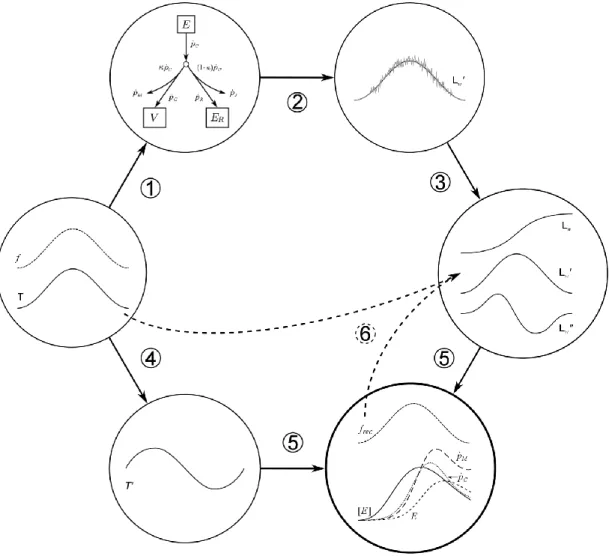
Fig. 1. Conceptual scheme of the validation procedure of the reconstruction process. (1) Artificially created
temperature and functional response time series are used as input for a standard DEB model; (2) noise is added to
the obtained growth trajectory (𝑳𝒘′) to mimic actual data; (3) the growth trajectory is smoothed using the “DEB
box” method and then integrated to obtain a length trajectory (𝑳𝒘) and derived to obtain the acceleration of growth
(𝑳𝒘′′); (4) the first derivative of temperature (𝑻′) is calculated; (5) the functional response 𝒇 and the DEB model
dynamics are reconstructed using the DEB Linear Equation; (6) the reconstructed 𝒇 and the initial temperature time series are used in a backward checking simulation to simulate the growth trajectory produced in step (3).
7
We created temperature and food availability time series commonly encountered by scallops in the middle of its distribution range: temperatures of 7–21 °C and a scaled functional response of 0.1– 0.9following a seasonal sinusoidal pattern. These time-series were used as forcing variables in the scallop DEB model (step 1 in Fig. 1) and a data set of daily shell growth rate was generated (𝐿𝑤′, the prime
notation being used as growth rates are derivatives of length). The initial conditions of the DEB model state variables were as described in Lavaud et al. (2014), with an initial length of 1.5 cm, an initial proportion of reserve fixed to 0.08% and initial mass fixed to 0.25 gDW (gram Dry Weight). Before applying the reconstruction procedure, artificial additive white Gaussian noise was applied to this growth trajectory (step 2 in Fig. 1) in order to mimic the combined effect of shell increments measurement error (Chauvaud et al., 1998) and natural high-frequency variability of daily growth (due to other factors than temperature and food). Two levels of noise were tested to evaluate the impact on the reconstruction method: a low amplitude of 50 µm d–1 and a high amplitude of 100 µm d–1. Root Mean Square Error (RMSE) was calculated to compare original and reconstructed functional response at the different noise levels. Because reliable striae identification is usually impossible for increments smaller than 50 µm (Chauvaud et al., 1998), noise was only applied to values above this threshold. Because the reconstruction procedure makes use of the derivative of growth rates, the high frequency variations of growth trajectories first need to be smoothed (step 3 in Fig. 1). Finally, after deriving the temperature (step 4 in Fig. 1), the reconstruction process was applied to reconstruct the functional response as well as the DEB model dynamics and fluxes (step 5 in Fig. 1). As a means to check the reliability of the procedure, the reconstructed 𝑓 and the temperature time series were used in a regular DEB simulation and the resulting growth compared to the original growth trajectory (step 6 in Fig. 1).
2.3.2. Data smoothing
Several algorithms were tested in order to smooth growth time series: a simple moving average, a weighted moving average (with weights that decreased linearly from the window center), an exponential moving average, and a polynomial moving average. We also tested the application of a low-pass filter: the Savitzky-Golay filter (Persson and Strang, 2003; performed using the “sgolayfilt" function of the Signal package for Octave v. 3.6.4). The rationale for using this method is that in addition to smoothing the signal, it gives direct access to the derivative of 𝐿𝑤′ (i.e. 𝐿𝑤′′), also required for the reconstruction of 𝑓. This smoothing method uses a regression based on the minimization of least squares differences to estimate a third degree polynomial that better fit the data. RMSE was calculated to compare the smoothed trajectories to the original growth time series.
As the major part of the high-frequency variations of scallop growth trajectories originates from the measurement process, we developed another smoothing approach based on DEB predicted daily growth potential. This method will hereafter be referred to as the "DEB box" method and works as follows: at each time step of the actual trajectory, growth was predicted through a DEB model with 𝑓 = 1 (maximum growth) and 𝑓 = 0 (minimum growth). The daily growth potential was bound to the maximal and minimal incremental growth laid down by the DEB predictions in order to ensure that the reconstructed 𝑓 stays within a plausible variation range (not due to observation error).
Observations of brutal drops in scallop shell growth have often been reported and were linked to feeding cessation, induced by toxic algae blooms or overloads of microalgae clogging scallop's gills (Chauvaud et al., 1998; Lorrain et al., 2000; Chauvaud et al., 2001). In order to investigate the potential of
8
the reconstruction procedure to retrace these “starvation” events, artificial breaks were inserted in the functional response function (𝑓) created at the beginning of the procedure (step 1 of Fig. 1). Different starvation durations, which created more or less marked drops in the resulting growth time series, were applied to test the resolution of the smoothing methods.
2.3.3. Data interpolation
In first trials, because the derivative of growth 𝐿𝑤′′ (i.e. its acceleration) is a parameter of the
reconstruction equation, we interpolated the growth trajectory in order to conduct the reconstruction calculations at a smaller time step (justified by the use of the acceleration of growth). Three interpolation methods were tested: a cubic spline, a linear method, and a polynomial Hermite method. The cubic spline and Hermite methods also give access to the derivative of growth (𝐿𝑤′′), which could easily and directly
be used in the DEB Linear Equation next. However, the interpolation of growth trajectories prior to run the equation was not conclusive. Highly unstable and out of range reconstructed 𝑓 resulted from the use of Hermite interpolation (Fig. S1a), while interpolating growth data with a cubic spline, although giving satisfactory backward simulation of growth, produced a reconstructed 𝑓 varying beyond its definition range (between 0 and 1, Fig. S1c). We interpreted these results as a consequence of the fact that the DEB Linear Equation calculates a value of 𝑓 corresponding to a given variation of 𝐿𝑤, 𝐿𝑤′, and 𝐿𝑤′′ between
two time steps. When interpolating, the “adaptation possibilities” of 𝑓 to the next step values of 𝐿𝑤, 𝐿𝑤′,
and 𝐿𝑤′′ are reduced as time step decreases. In other words, the value of 𝑓 can vary more freely within long time steps than in short ones, as long as it produces the expected variable values at the next time step. Interpolating growth trajectories to a time step smaller than the day was therefore abandoned. The functional response was reconstructed at a daily time step and then smoothed using a Savitzky-Golay filter (similar results were obtained with a moving average with weighting coefficients linearly decreasing from the window center).
2.3.4. Other reconstructed variables
Reserve 𝐸, reserve density [𝐸], mobilization flux 𝑝̇𝐶, and maintenance flux 𝑝̇𝑀 were reconstructed through Eq. 3 to 6. A first test was performed using a smooth growth trajectory (no added noise). In a second test growth trajectories with added noise where used after being filtered by the "DEB box" method. As the resulting time series still presents rather abrupt variations, the reconstructed DEB dynamics and fluxes were smoothed using a Savitzky-Golay filter (smoothing window: 30 days).
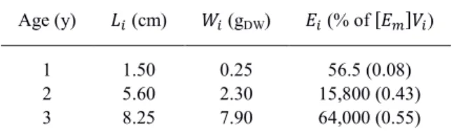
Finally, simulations using different initial shell lengths were performed to check for any effect of initial size conditions: the first (juvenile), second, and third year of growth were simulated using initial conditions presented in Table 2.
Table 2. Initial conditions of the simulations starting at age 1, 2 and 3: initial length 𝐿𝑖, initial dry weight 𝑊𝑖, initial
reserves 𝐸𝑖 (percentage of the volume specific maximum energy density, [𝐸𝑚]𝑉𝑖).
Age (y) 𝐿𝑖 (cm) 𝑊𝑖 (gDW) 𝐸𝑖 (% of [𝐸𝑚]𝑉𝑖)
1 1.50 0.25 56.5 (0.08)
2 5.60 2.30 15,800 (0.43)
9
3. Results
3.1. Smoothing methods for growth times series
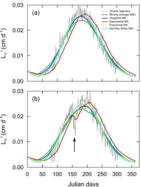
The different algorithms used to artificially smooth noise in theoretical growth times series are presented in Fig. 2a. The size of the averaging window was calibrated at 31 days when using moving averages and at 151 days for the Savitzky-Golay method. In both cases, the smoothing interval decreased at the extremities of the growth time series in order to keep symmetric smoothing windows.
Fig. 2. Different algorithms used to smooth artificially noisy growth trajectories (gray line), with (a) a simple
seasonal growth time series as initial functional response and (b) a forced stop in assimilation (arrow). Moving average (green line), moving average with weighting coefficients linearly decreasing from the window center (blue line), exponential moving average (red line), polynomial moving average (yellow line) with a smoothing window of
31 days and Savitzky-Golay filter with a smoothing window of 151 days (cyan line) were tested.
The use of a simple moving average did not produce acceptable results (although RMSE was relatively low: 0.0020 cm d–1). The smoothed curve was below many of the original points in the central part of graph, which could be fixed by reducing the smoothing window length. Nevertheless, small variations were still observed, due to the narrow smoothing window, likely to produce highly fluctuating derivatives that compromise the application of the DEB Linear Equation. This first option was therefore abandoned. Noticeable degradation occurred at both ends of the smoothed curve when using an exponential moving average (RMSE = 0.0028 cm d–1). Linearly decreasing weighting coefficients from the window center was satisfying (RMSE = 0.0016 cm d–1). Polynomial smoothing also showed good results although visible degradation occurred at the extremities of the growth trajectory (RMSE = 0.0014 cm d–1). The Savitzky-Golay filter was also conclusive, especially at the extremities (first and last twenty days) where the averaged curve was not as impacted by the last points as compared to the moving averages (RMSE = 0.0014 cm d–1).
10
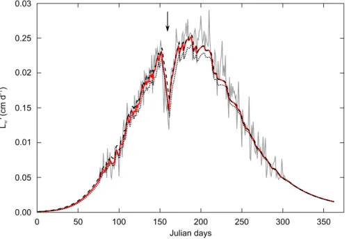
When inserting an artificial and brutal starvation of seven days in the food input, leading to a decrease of growth rate (Fig. 2b) all methods strongly reduced or made the growth stop vanish, irrespective of the size of the smoothing window used. The "DEB box" method, however, succeeded in keeping track of this event in the resulting dynamics while constraining it to a variation range compatible with DEB predictions (Fig. 3). The constrained growth curve still presented a saw-tooth shape as the "DEB box" filter only bounds the signal to vary between 0 and 1 when observed growth overshoots DEB predictions. Therefore, the reconstructed 𝑓 would still highly fluctuate. Nevertheless, after smoothing the reconstructed data (using a Savitzky-Golay filter), the model was able to simulate the original 𝑓 time series (see further results in following section). As the "DEB box" method was the more robust way to eliminate the high-frequency variations of growth trajectory it was selected for the rest of the study.
Fig. 3. The "DEB box" method used to smooth a typical growth trajectory with an assimilation stop (arrow): for
each point of the initial growth trajectory (gray line), predictions of growth compatible with DEB predictions were made for the next time step. Predicted growth was calculated for 𝒇 = 1 (dashed dark line) and for 𝒇 = 0 (dotted dark
line), to define the variation range of growth allowed by DEB theory. If initial growth trajectory was out of these bounds, the smoothed time series was set at the value given by the DEB model. If initial growth trajectory fitted
inside DEB predictions, its value was kept unchanged. The resulting curve is in red.
3.2. Reconstructing the functional response
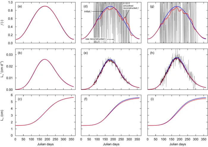
In the simple case of a smooth growth (no added noise), the functional response simulated from temperature and length increments exactly overlapped the original 𝑓 used to produce the growth trajectory (Fig. 4, left panels). Backward simulation of growth using the reconstructed 𝑓 to check for inconsistency in the process revealed a close to perfect reproduction of the original growth time series. When artificial noise was randomly added to the initial growth trajectory (Fig. 4, middle and right panels) results of both reconstruction and backward simulation, though not as faithful, were very satisfying. The level of noise seemed to have a low impact the accuracy of the reconstruction method as the RMSE of reconstructed functional response was similar at both level tested: 0.05 for the lower noise amplitude
11
(Fig. 4d) and 0.07 for the higher noise amplitude (Fig. 4g). However, back simulated shell length tended to be slightly lower than the original time series when artificial noise was added (Fig. 4f,i).
3.3. Reconstruction of assimilation stops
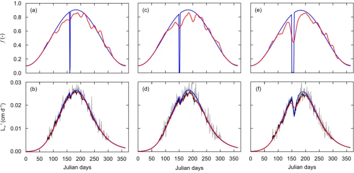
The duration of assimilation stops tested to evaluate the resolution of the smoothing method showed that growth trajectories were not impacted by a starvation of 24 h (Fig. 5b). Growth rate started to decrease when starvation lasted for three days and clearly slowed down over seven days (Fig. 5d,f). In the reconstruction of 𝑓 dynamics, apparent curve inflections were observed for three and seven days of starvation only.
Fig. 4. Reconstruction of assimilation trajectory from intact (a, b, c) and artificially noisy growth data: 50 µm d–1
amplitude (d, e, f); 100 µm d–1 amplitude (g, h, i). Upper panels: initial 𝒇 trajectory (blue line), raw reconstructed 𝒇
(gray line) and smoothed reconstructed 𝒇 using a Savitzky-Golay filter (red line). Center panels: initial intact growth trajectory (blue line), noisy growth trajectory (e, gray line), smoothed growth trajectory using the "DEB box" method (dark line) and backward simulation using smoothed reconstructed 𝒇 (red line). Lower panels: initial shell
12
3.4. Reconstructing physiological history
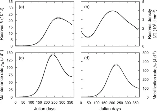
As expected, the reconstruction of DEB dynamics and fluxes from smooth growth trajectories (no added noise) perfectly overlapped the curves produced with the standard DEB model (results subsequently not shown). This validates the use of the DEB Linear Equation as a reconstruction tool of these dynamics. The high frequency variability of artificially noisy growth data impacted the reconstructed reserve 𝐸 (Fig. 6a), reserve density [𝐸] (Fig. 6b), and mobilization flux 𝑝̇𝐶 (Fig. 6d) but had no effect on the somatic maintenance flux 𝑝̇𝑀 (Fig. 6c). The smoothing applied to the reconstructed dynamics and fluxes (Savitzky-Golay filter) produced very good results as the smoothed curves fitted well the original dynamics of 𝐸, [E], and 𝑝̇𝐶 (Fig. 7).
3.4. Effect of shell size
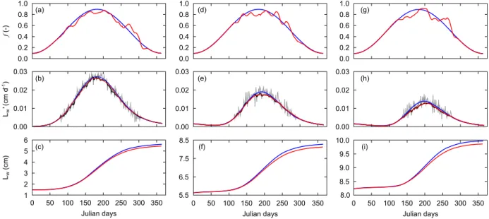
Finally, the main effect observed in older individuals was a shorter duration of growth, which resulted in a reduction of the reconstruction window (Fig. 8). The amplitude range of growth was also lower in older organisms, reaching 75 µm d–1 (Fig. 8c), whereas the juvenile shell could grow at a rate up to 300 µm d–1 (Fig. 8c). Nevertheless, the ability of the DEB Linear Equation to reconstruct the functional response was not affected.
Fig. 5. Reconstruction of 𝒇 from artificially noisy growth data in three scenarios of assimilation cessation lasting one day (left), three days (center) and seven days (right). Upper panels: initial (blue line) and reconstructed 𝒇 (red line). Lower panels: growth trajectories generated using the initial 𝒇 (blue line) to which noise was added (gray line)
were smoothed using the "DEB box" method (dark line) and used in the reconstruction procedure. Backward simulation of growth rate (red line) used the reconstructed 𝒇, smoothed with the Savitzky-Golay filter.
13
Fig. 6. DEB variables calculated from the DEB Linear Equation using an artificially noisy growth trajectory. Gray
lines indicate the variables as predicted by the standard DEB model used to produce the growth trajectory. Dark
lines indicate the predictions for (a) Reserve energy 𝑬 (J), (b) reserve density [𝑬] (J cm–3), (c) somatic maintenance
flux 𝒑̇𝑴 (J d–1), and (d) mobilization flux 𝒑̇𝑪 (J d–1).
Fig. 7. DEB variables calculated from the DEB Linear Equation using an artificially noisy growth trajectory. (a)
Reserve energy 𝑬 (J), (b) reserve density [𝑬] (J cm–3), (c) somatic maintenance flux 𝒑̇
𝑴 (J d–1), and (d) mobilization
flux 𝒑̇𝑪 (J d–1). Gray lines indicate variables as predicted by the standard DEB model used to produce growth
14
Fig. 8. Reconstruction of functional response 𝒇 from theoretical growth rates of one-year-old (left panels), two-year-old (middle panels) and three-year-two-year-old (right panels) shells of Pecten maximus. (a, d, g) Initial 𝒇 (blue line) and reconstructed 𝒇 (red line). (b, e, h) Artificial noise (gray line) was added to initial growth trajectories (blue line), which were smoothed using the "DEB box" method (dark line). Backward simulations of daily shell growth rate (b,
e, h) and shell length (c, f, i) using smoothed reconstructed 𝒇 are indicated in red lines.
4. Discussion
Accurate and reliable assessment of what organisms eat in nature will always be difficult. In this study we presented a method to address this issue through bioenergetics modelling. The approach is based on an inverted Dynamic Energy Budget model and allows the reconstruction of the assimilated energy as well as physiological variables dynamics from growth trajectories. We successfully applied this innovative technique to the case of a bivalve using growth increments of its shell.
4.1. Inversion of the DEB model
Only few studies have attempted to reconstruct feeding dynamics using DEB models. Cardoso et al. (2006) were the first to reconstruct mean functional responses of five bivalve species from annual growth data in Dutch coastal waters. In a simple empirical way, the reconstructed 𝑓 was manually calibrated to match the observed growth of these bivalves. Then, Freitas et al. (2009) extended these investigations to a wider latitudinal range for North-East Atlantic coastal bivalve species. Their approach was based on a regression routine (non-linear weighted least-squares regression using Nelder Mead's simplex method) to estimate the functional response given annual temperature cycles and observed length-at-age data. According to their simulations, the assimilation capacities of the studied bivalves were all limited to a maximum of 70% (reconstructed 𝑓 < 0.7). The method described by Kooijman (2010) makes the assumption that (the mean) food density changes slowly enough to allow an approximation of energy reserve 𝑒 = 𝑓. Rapid changes of seston abundance and composition, especially in coastal ecosystems, can therefore be missed in the reconstructed feeding activity. More recently, Pecquerie et al. (2012) developed
15
an inverted DEB model for reconstructing scaled food density trajectories and growth history of anchovy, using opacity data of fish otoliths. Their reconstruction procedure was defined as the determination of the feeding values minimizing the square deviation between the observed and the predicted opacity values. These authors, while presenting promising results in theoretical cases, did report a low sensitivity of their method to temperature variations experienced by the organism.
The novelty of the present study is that the reconstruction of the functional response is not based on a fitting procedure but on an equation. Moreover, few parameters are required to perform the simulations. Since this study is the first study to present an application of Rannou’s (2009) DEB Linear Equation, various tests had to be conducted before an application to real data. In the testing procedure, we imposed a supplementary difficulty adding noise to the theoretical data, in the view of producing "pseudo-real data". Yet, even then, the reconstruction process produced a very satisfactory reconstruction of the initial assimilation dynamics. This scrambling step is not often encountered in the literature and theoretical studies usually settle for simpler scenarios.
4.2. Treatment of growth trajectories
The growth of the great scallop and other bivalves can be measured at a daily scale thanks to the incremental growth of the shell. Other organisms, such as fish used to determine growth rate that could be used to reconstruct food availability and physiological state. Nevertheless, daily growth rate data are not always as easy to collect and while the use of interpolation methods should permit the application of the model inversion procedure, the obtained predictions would reflect the frequency of growth trajectory data points.
A common issue encountered in sclerochronology is the high-frequency variability of growth rate data, especially in bivalves. Despite a statistically rigorous procedure of growth trajectory treatment, the method proposed by Chauvaud et al. (1998) can still result in data sets with high-frequency fluctuations because measurement are generally done on a restricted number of individuals. Nevertheless, most of these variations might not have any biological significance (simply due to the accuracy/variability of the observation of growth increments). In the previously cited studies dealing with reconstruction of food assimilation trajectories from growth observations (Cardoso et al., 2006; Freitas et al., 2009; Troost et al., 2010; Pecquerie et al., 2012), the uncertainty or the variability of growth data measurement was a recurring issue. Cubic splines were globally used and advised for smoothing observed growth data variability (Freitas et al., 2009; Kooijman, 2010). However, this interpolation method used to smooth data has the disadvantage of producing highly variable derivative of growth rates, which causes the reconstructed trajectory to overshoot its accepted variation range (Freitas et al., 2009). This was even more problematic in the development of the current method as the DEB Linear Equation makes use of second derivatives of length (𝐿𝑤′′) which then can cause the reconstructed 𝑓 to go beyond its possible range (0–1).
The "DEB box” method developed in this work was designed to eliminate the variability due to observation and to constrain the evolution of observed growth trajectories to a variation range compatible with DEB predictions at each time step. With the use of the "DEB box" approach, observed growth data of varying intensity of high-frequency variations did not require smoothing processes any longer (Fig. 4). The fact that raw reconstructed 𝑓 time series were highly variable is not aberrant as reconstruction was
16
carried out at a short time step. Biologically, however, assimilation flux is a rather smooth process at a daily scale compared to feeding activity. Therefore, the smoothing of the reconstructed 𝑓 before the backward simulation was justified and allowed getting closer to a real assimilation time series. The discrepancies sometimes observed at the end of the simulations may not be due to the smoothing method alone (Savitzky-Golay filter). This could result from the artificial noise (a well-known effect in kernel smoothing), added at a period during which natural variations are usually less pronounced (low temperature and food availability). This might cause slight and temporary overestimations when using real data and one should be cautious in the interpretation of the reconstructed assimilation time series when approaching the extremity of growth trajectory.
Generally the reconstruction of past physiological or environmental conditions is more valuable when the archive used covers a long period of time. However, after four (in southern populations) to six (in northern populations) years of life, great scallops barely produce more than a few millimeters of shell each year, while then can gain up to 4 cm during the second year of growth (Chauvaud et al., 2012). Growth during the last years of life is dramatically reduced, both in duration and in amplitude, which makes it difficult to analyze. The results presented in Fig. 8 also reveal that the reconstructed assimilation dynamics are a bit less accurate during the third year of growth, compared to the first or the second. Therefore, it would be recommended to use young individuals to reconstruct assimilation history.
4.3. Reconstructing physiological state
The present method does not only allow the reconstructing the feeding activity but also the physiological history of the studied organism. Although the fitting of a complete model can produce such estimates of physiological variables (maintenance, reserve density, etc.), the approach described in this study requires substantially less parameters (8 at maximum). Based on the growth trajectories and knowing the temperature experienced by the organism, it was possible to reconstruct the dynamics of reserve or the amount of energy used in maintenance of somatic tissues. Predictions of these variables reflected the high-frequency variability of growth when observed, giving another evidence of the reliability of the method. As expected, the somatic maintenance flux was not impacted by growth variability, as it is directly linked to structural volume (𝑝̇𝑀= [𝑝̇𝑀]𝑉). The reserve compartment acts as a buffer of
environmental variability, smoothing out rapid changes and allowing organisms to survive starvation periods for a while (Pecquerie et al., 2009; Lavaud et al., 2014). As a result, it is easier to reconstruct the somatic maintenance than the state of reserve and its dynamics at a point in time, the former depending on structural volume and the later depending on reserve state. This type of reconstruction is of great interest for a number of study fields: paleo-reconstruction, ecophysiology, assessment of pollutions, of diseases, creation of distribution maps, and characterization of the carrying capacity of habitats.
In this study the reproductive part of the DEB model was not considered. Nevertheless, the dynamics of the reproduction buffer are easily related to growth thanks to the 𝜅-rule. As it is now possible to reconstruct the reserve dynamics, the dynamics of energy allocated to maturity and reproduction could be reconstructed.
17
4.4. Perspectives and further research
This approach offers great perspectives to better understand energetic patterns behind observed life history traits of bivalves. Scallop shell collections exist in many research centers along its geographical distribution range (in the University of Brest, France; the University of Bangor, Wales; the Institute of Marine Research of Bergen, Norway); the exploration of such archives could aid comprehension of the physiology of this species and its remarkable growth and reproductive pattern throughout its distribution area. Moreover, it could be used to study remote populations such as those living on the continental shelf (Nérot et al., 2012) and for which little information is available. In a following article published in this issue, Lavaud et al. (2018) undertook the application of the reconstruction method to answer these questions and brought new insights on the latitudinal and bathymetric trends observed in P. maximus along its distribution area.
High-resolution biogenic archives of environmental conditions such as the calcified tissues of bivalve mollusks can significantly increase our knowledge of seasonal to multi-decadal paleoclimate and paleoenvironmental variability (Schöne and Gillikin, 2013). The perspective of reconstructing past environmental conditions through sclerochronology together with the organism's physiological history is exciting, especially in the context of climate change. Moreover, confronting the reconstructed physiological history of a biogenic archive to the quantified proxy data measured in sclerochronological records might help addressing the adverse influence of vital effects on the proxy records (Schöne and Gillikin, 2013). Finally, the reconstruction method presented in this study could be of high interest in some paleontology studies, which aim at reconstructing the physiology of ancient organisms, by providing an alternative to altered isotopic compositions from fossilisation processes (Kolodny et al., 1996).
Acknowledgements: The authors want to thank Starrlight Augustine and one anonymous reviewer for their helpful comments on the manuscript. This work benefited from funding provided by the COMANCHE program (ANR-2010-STRA-010).
Supplementary Material
Available at the end of this document.
Submitted: 14 December 2017
Received in revised form: 22 June 2018 Accepted: 08 July 2018
18
References
Aguirre Velarde, A., Flye-Sainte-Marie, J., Mendo, J. and Jean, F. (2015). Sclerochronological records and daily microgrowth of the Peruvian scallop (Argopecten purpuratus, Lamarck, 1819) related to environmental conditions in Paracas Bay, Pisco, Peru. J. Sea Res. 99, 1–8.
Antoine, L. (1978). La croissance journalière chez Pecten maximus (L.)(Pectinidae, Bivalvia). Daily growth of Pecten maximus (L.)(Pectinidae, Bivalvia). Haliotis 9, 627–636.
Barats, A., Amouroux, D., Pécheyran, C., Chauvaud, L. and Donard, O.F.X. (2008). High-frequency archives of manganese inputs to coastal waters (Bay of seine, France) resolved by the LA-ICP-MS analysis of calcitic growth layers along scallop shells (Pecten maximus). Environ. Sci. Technol. 42 (1), 86–92.
Bartell, S.M., Breck, J.E., Gardner, R.H. and Brenkert, A.L. (1986). Individual parameter perturbation and error analysis of fish bioenergetics models. Can. J. Fish. Aquat. Sci. 43 (1), 160–168.
Bourlès, Y., Alunno-Bruscia, M., Pouvreau, S., Tollu, G., Leguay, D., Arnaud, C., Goulletquer, P. and Kooijman, S.A.L.M. (2009). Modelling growth and reproduction of the Pacific oyster Crassostrea gigas: advances in the oyster-DEB model through application to a coastal pond. J. Sea Res. 62 (2–3), 62–71.
Cardoso, J.F.M.F., Witte, J.I.J. and van der Veer, H.W. (2006). Intra- and interspecies comparison of energy flow in bivalve species in Dutch coastal waters by means of the Dynamic Energy Budget (DEB) theory. J. Sea Res. 56 (2), 182–197.
Chauvaud, L., Thouzeau, G. and Paulet, Y.-M. (1998). Effects of environmental factors on the daily growth rate of Pecten maximus juveniles in the Bay of Brest (France). J. Exp. Mar. Biol. Ecol. 227 (1), 83–111.
Chauvaud, L., Donval, A., Thouzeau, G., Paulet, Y.-M. and Nézan, E. (2001). Variations in food intake of Pecten maximus (L.) from the Bay of Brest (France): Influence of environmental factors and phytoplankton species composition. C. R. Acad. Sci. Series III 324 (8), 743–755.
Chauvaud, L., Lorrain, A., Dunbar, R.B., Paulet, Y.-M., Thouzeau, G., Jean, F., Guarini, J.-M. and Mucciarone, D. (2005). Shell of the great scallop Pecten maximus as a high-frequency archive of paleoenvironmental changes. Geochem. Geophys. Geosyst. 6, Q08001.
Chauvaud, L., Patry, Y., Jolivet, A., Cam, E., Le Goff, C., Strand, Ø., Charrier, G., Thébault, J., Lazure, P., Gotthard, K. and Clavier, J. (2012). Variation in size and growth of the great scallop Pecten maximus along a latitudinal gradient. PLoS One 7 (5), e37717.
Chipps, S.R. and Wahl, D.H. (2008). Bioenergetics modeling in the 21st century: reviewing new insights and revisiting old constraints. Trans. Am. Fish. Soc. 137 (1), 298–313.
Clark, G.R. (1968). Mollusk shell: daily growth lines. Science 161 (3843), 800–802.
Eaton, J.W., Bateman, D., Hauberg, S. and Wehbring, R. (2016). GNU Octave version 4.2.0 manual: a high-level interactive language for numerical computations.
Flye-Sainte-Marie, J., Jean, F., Paillard, C., Ford, S. E., Powell, E., Hofmann, E. and Klinck, J. (2007). Ecophysiological dynamic model of individual growth of Ruditapes philippinarum. Aquaculture 266 (1–4), 130– 143.
Freitas, V., Cardoso, J.F.M.F., Santos, S., Campos, J., Drent, J., Saraiva, S., Witte, J.I.J., Kooijman, S.A.L.M. and van der Veer, H.W. (2009). Reconstruction of food conditions for northeast Atlantic bivalve species based on dynamic energy budgets. J. Sea Res. 62 (2–3), 75–82.
Furness, R.W. (1978). Energy requirements of seabird communities: a bioenergetics model. J. Anim. Ecol. 47, 39– 53.
19
Grant, J. and Bacher, C. (1998). Comparative models of mussel bioenergetics and their validation at field culture sites. J. Exp. Mar. Biol. Ecol. 219 (1–2), 21–44.
Kolodny, Y., Luz, B., Sander, M. and Clemens, W.A. (1996). Dinosaur bones: fossils or pseudomorphs? The pitfalls of physiology reconstruction from apatitic fossils. Palaeogeogr. Palaeoclimatol. Palaeoecol. 126(1–2), 161–171. Kooijman, S.A.L.M. (2010). Dynamic Energy Budget Theory for Metabolic Organization. Cambridge, UK, third edition. University Press, 532 pp.
Laing, I. (2000). Effect of temperature and ration on growth and condition of king scallop Pecten maximus spat. Aquaculture 183 (3–4), 325–334.
Laing, I. (2002). Effect of salinity on growth and survival of king scallop spat Pecten maximus. Aquaculture 205 (1– 2), 171–181.
Lavaud, R., Thébault, J., Lorrain, A., van der Geest, M. and Chauvaud, L. (2013). Senilia senilis (Linnaeus, 1758), a biogenic archive of environmental conditions on the Banc d’Arguin (Mauritania). J. Sea Res. 76, 61–72.
Lavaud, R., Flye-Sainte-Marie, J., Jean, F., Emmery, A., Strand, Ø. and Kooijman, S.A.L.M. (2014). Feeding and energetics of the great scallop, Pecten maximus, through a DEB model. J. Sea Res. 94, 5–18.
Lavaud, R., Jolivet, A., Rannou, E., Jean, F., Strand, Ø. and Flye-Sainte-Marie, J. (2018). What can the shell tell about the scallop? Using growth trajectories along latitudinal and bathymetric gradients to reconstruct physiological history with DEB theory. J. Sea Res. (in press, this issue).
Liu, H., Kelly, M.S., Campbell, D.A., Fang, J. and Zhu, J. (2008). Accumulation of domoic acid and its effect on juvenile king scallop Pecten maximus (Linnaeus, 1758). Aquaculture 284 (1–4), 224–230.
Lorrain, A., Paulet, Y.-M., Chauvaud, L., Savoye, N., Nézan, E. and Guérin, L. (2000). Growth anomalies in Pecten maximus from coastal waters (Bay of Brest, France): relationship with diatom blooms. J. Mar. Biol. Assoc. UK 80 (4), 667–673.
Marques, G.M., Augustine, S., Lika, K., Pecquerie, L., Domingos, T. and Kooijman, S.A.L.M. (2018). The AmP project: Comparing species on the basis of dynamic energy budget parameters. PLoS Comput. Biol. 14(5), p.e1006100.
Nérot, C., Lorrain, A., Grall, J., Gillikin, D.P., Munaron, J.-M., Le Bris, H. and Paulet, Y.-M. (2012). Stable isotope variations in benthic filter feeders across a large depth gradient on the continental shelf. Estuar. Coast. Shelf Sci. 96, 228–235.
Owen, R., Richardson, C. and Kennedy, H. (2002). The influence of shell growth rate on striae deposition in the scallop Pecten maximus. J. Mar. Biol. Assoc. UK 82, 621–623.
Pecquerie, L., Petitgas, P. and Kooijman, S.A.L.M. (2009). Modeling fish growth and reproduction in the context of the Dynamic Energy Budget theory to predict environmental impact on anchovy spawning duration. J. Sea Res. 62 (2–3), 93–105.
Persson, P.-O. and Strang, G. (2003). Smoothing by Savitzky-Golay and Legendre filters. In Mathematical Systems Theory in Biology, Communications, Computation, and Finance. Joachim Rosenthal and David S. Gilliam eds., pp. 301–315.
Picoche, C., Le Gendre, R., Flye-Sainte-Marie, J., Françoise, S., Maheux, F., Simon, B. and Gangnery, A. (2014). Towards the Determination of Mytilus edulis Food Preferences Using the Dynamic Energy Budget (DEB) Theory. PloS One 9(10), e109796.
Rannou, E. (2009). Discovering and learning DEB theory through the Growth DEB equation. In: DEB Theory Symposium 2009: 30 years of research for metabolic organization. Brest, France, 19–22 April 2009.
20
Schöne, B.R. and Gillikin, D.P. (2013). Unraveling environmental histories from skeletal diaries–advances in sclerochronology. Palaeogeogr. Palaeoclimatol. Palaeoecol. 373, 1–5.
Stockwell, J.D. and Johnson, B.M. (1997). Refinement and calibration of a bioenergetics based foraging model for kokanee (Oncorhynchus nerka). Can. J. Fish. Aquat. Sci. 54 (11), 2659–2676.
Thébault, J. and Chauvaud, L. (2013). Li/Ca enrichments in great scallop shells (Pecten maximus) and their relationship with phytoplankton blooms. Palaeogeogr. Palaeoclimatol. Palaeoecol. 373, 108–122.
Troost, T.A., Wijsman, J.W.M., Saraiva, S. and Freitas, V. (2010). Modelling shellfish growth with dynamic energy budget models: an application for cockles and mussels in the Oosterschelde (Southwest Netherlands). Phil. Trans. R. Soc. B Biol. Sci. 365 (1557), 3567–3577.
21
SUPPLEMENTARY MATERIAL
Part I – Development of the DEB Linear Equation
The development of the DEB linear equation by Rannou (2009) emerged from an attempt to make DEB modelling more accessible to answering basic questions related to growth patterns among organisms. It is a simplification of the original set of equations required to perform DEB simulations, using less parameters and focussing on two state variables (structure 𝑉 and reserve 𝐸). The third state variable considered in the standard DEB model, the reproduction buffer 𝐸𝑅, relates mechanically to the energy extracted from 𝐸 through the 𝜅-rule and can therefore be omitted.
We start by showing that the DEB model dynamics (without considering maturation) is equivalent to the following system of differential equations:
{
3[𝐸𝐺]𝐿3𝐿′= 𝜅𝜐̇𝐸 − 3𝜅𝐸𝐿′− [𝑝̇
𝑀]𝐿4 (A1)
𝐸′𝐿 = {𝑝̇
𝐴𝑚}𝑓𝑉 − 𝜐̇𝐸 + 3𝐸𝐿′ (A2)
The first equation can be deducted from the following reasoning. The so-called 𝜅-rule splits 𝑝̇𝐶, the utilization flow of energy from 𝐸, into somatic and maturation branches:
𝜅𝑝̇𝐶 = 𝑝̇𝐺+ 𝑝̇𝑆 (A3) (1 − 𝜅)𝑝̇𝐶 = 𝑝̇𝑅+ 𝑝̇𝐽 (A4)
with 𝑝̇𝐺 the flow to somatic growth, 𝑝̇𝑆 the flow to somatic maintenance, 𝑝̇𝑅 the flow to maturation and reproduction and 𝑝̇𝐽 the flow to maturity maintenance. Growth is there defined by:
𝑑𝐿
𝑑𝑡 = 𝐿′ = 𝑝̇𝐺
3𝐿2[𝐸
𝐺] (A5)
from which the flux of energy allocated to growth is obtained: 𝑝̇𝐺 = 3𝐿2[𝐸𝐺]𝐿′. And with:
𝑝̇𝑆= 𝑝̇𝑀+ 𝑝̇𝑇 = [𝑝̇𝑀]𝐿3+ {𝑝̇
𝑇}𝐿2 (A6)
We now have in Eq. (A3):
𝜅𝑝̇𝐶 = 3𝐿2[𝐸
𝐺]𝐿′+ [𝑝̇𝑀]𝐿3+ {𝑝̇𝑇}𝐿2 (A7)
In the case of ectotherms, {𝑝̇𝑇} = 0, so we can write:
3𝐿2[𝐸
𝐺]𝐿′= 𝜅𝑝̇𝐶− [𝑝̇𝑀]𝐿3 (A8)
Different expressions of 𝑝̇𝐶 have been published (Kooijman, 2010; Bernard et al., 2011; Jusup et al., 2017), a simple way to express this flux is:
22 𝑝̇𝐶 = [𝐸] (𝜐̇𝐿2−𝑑𝐿3 𝑑𝑡 ) = 𝐸 𝐿3(𝜐̇𝐿2− 3𝐿2𝐿′) = 𝐸 𝐿(𝜐̇ − 3𝐿′) (A9) By replacing this expression of 𝑝̇𝐶 in Eq. (A3) and multiplying by 𝐿 we arrive to Eq. (A1).
The dynamics of reserves in DEB theory is given by: 𝑑𝐸
𝑑𝑡 = 𝐸′= 𝑝̇𝐴− 𝑝̇𝐶 (A10) in which the assimilation flux 𝑝̇𝐴= {𝑝̇𝐴𝑚}𝑓𝐿2. Eq. (A2) is obtained by inserting Eq. (A9) in Eq. (A10)
and multiplying by 𝐿.
The concept of a linear equation to describe DEB variables dynamics requires that the two state variables 𝐸 and 𝐿 be replaced by 𝐿𝑤 and its derivative 𝐿𝑤′ in the differential system. The sequence of steps to
achieve this is first to derive Eq. (A1), from which 𝐸′ is eliminated using eq. (A2), and then 𝐸 is eliminated using Eq. (A1). As the parameters [𝑝̇𝑀] and 𝜐̇ are affected by temperature through time, the obtained derivative of Eq. (A1) is:
9[𝐸𝐺]𝐿2𝐿′2+ 3[𝐸
𝐺]𝐿2𝐿′′ = 𝜅𝜐̇𝐸′ − 3𝜅𝐸′𝐿′ − 3𝜅𝐸𝐿′′ − 4[𝑝̇𝑀]𝐿3𝐿′ + 𝜅𝜐̇′𝐸 − [𝑝̇𝑀]′𝐿4 (A11)
After multiplication by 𝐿, the term 𝐸′𝐿 is replaced by Eq. (A2). And after multiplication by (𝜐̇ − 3𝐿′) the term 𝐸 is replaced by Eq. (A1) solved for 𝐸, leading to the equation:
−9𝜐̇[𝐸𝐺]𝐿′2+ 3𝜐̇[𝐸
𝐺]𝐿𝐿′′ − 𝜅𝜐̇2{𝑝̇𝐴𝑚}𝑓 + 6𝜅𝜐̇{𝑝̇𝐴𝑚}𝑓𝐿′ − 9𝜅{𝑝̇𝐴𝑚}𝑓𝐿′2
−2𝜐̇[𝑝̇𝑀]𝐿𝐿′ − 3[𝑝̇𝑀]𝐿𝐿′2+ 𝜐̇2[𝑝̇
𝑀]𝐿 + 3[𝑝̇𝑀]𝐿2𝐿′′ + 3𝜐̇2[𝐸𝐺]𝐿′
−([𝑝̇𝑀]𝐿 + 3[𝐸𝐺]𝐿′)𝜐̇′𝐿 + (𝜐̇ − 3𝐿′)[𝑝̇𝑀]′𝐿2= 0 (A12)
The next steps are simple substitutions of some terms of this formula. The structural length can be replaced by the physical length 𝐿𝑤, as 𝐿 = 𝐿𝑤𝛿𝑀.
The term 𝜅{𝑝̇𝐴𝑚} can be replaced by: 𝜅{𝑝̇𝐴𝑚} = 𝑘̇𝑀𝑔𝐿𝑚 𝜐̇ 𝜅{𝑝̇𝐴𝑚} = 𝜅{𝑝̇𝐴𝑚} 𝜐̇𝜅[𝐸𝑚][𝐸𝐺]𝑘̇𝑀𝐿𝑚= [𝐸𝐺]𝑘̇𝑀𝐿𝑚= [𝐸𝐺]𝑘̇𝑀𝐿𝑤𝑚𝛿𝑀 with 𝐿𝑚= 𝜐̇ 𝑘̇𝑀𝑔 , 𝑔 = [𝐸𝐺] 𝜅[𝐸𝑚] , and 𝜐̇ = {𝑝̇𝐴𝑚}
[𝐸𝑚]. Then the volume-specific somatic maintenance cost can be replaced by [𝑝̇𝑀] = [𝐸𝐺]𝑘̇𝑀. Then a division by 𝛿𝑀[𝐸𝐺] and the introduction of the shape corrected energy conductance 𝜐̇𝑤 = 𝜐̇
𝛿𝑀 leads to:
−9𝜐̇𝑤𝐿𝑤′2+ 3𝜐̇𝑤𝐿𝑤𝐿𝑤′′− 𝜐̇𝑤2𝑓𝑘̇𝑀𝐿𝑤𝑚+ 6𝑓𝜐̇𝑤𝑘̇𝑀𝐿𝑤𝑚𝐿𝑤′− 9𝑓𝑘̇𝑀𝐿𝑤𝑚𝐿𝑤′2
−2𝜐̇𝑤𝑘̇𝑀𝐿𝑤𝐿𝑤′− 3𝑘̇𝑀𝐿𝑤𝐿𝑤′2+ 𝜐̇𝑤2𝑘̇𝑀𝐿𝑤+ 3𝑘̇𝑀𝐿𝑤2𝐿𝑤′′+ 3𝜐̇𝑤2𝐿𝑤′
−(𝑘̇𝑀𝐿𝑤+ 3𝐿𝑤′)𝜐̇𝑤′𝐿𝑤+ (𝜐̇𝑤− 3𝐿𝑤′)𝑘̇𝑀′𝐿𝑤2 = 0 (A13)
23
temperature dependence of a physiological rate 𝑘̇ is well described by the Arrhenius relationship: 𝑘̇(𝑡) = 𝑘̇0𝑒−
𝑇𝐴
𝑇(𝑡) . The derivation of which is given by:
𝑘̇′(𝑡)= 𝑘̇ 0𝑒− 𝑇 𝐴 𝑇(𝑡)𝑇𝐴𝑇′(𝑡) 𝑇(𝑡)2 = 𝑘̇(𝑡) 𝑇𝐴𝑇′(𝑡) 𝑇(𝑡)2 (A14)
The terms 𝜐̇𝑤′ and 𝑘̇𝑀′ can now be replaced and after simplification and a division by a factor 𝜐̇𝑤, the DEBLE is obtained: −9𝐿𝑤′2+ 3𝐿𝑤𝐿𝑤′′− 𝑓𝜐̇𝑤𝑘̇𝑀𝐿𝑤𝑚+ 6𝑓𝑘̇𝑀𝐿𝑤𝑚𝐿𝑤′+ 3𝜐̇𝑤𝐿𝑤′+ 𝜐̇𝑤𝑘̇𝑀𝐿𝑤− 2𝑘̇𝑀𝐿𝑤𝐿𝑤′ −9𝑓𝑘̇𝑀𝐿𝑤𝑚 𝜐̇𝑤 𝐿𝑤′2− 3𝑘̇𝜐̇𝑀 𝑤𝐿𝑤𝐿𝑤′ 2+ 3𝑘̇𝑀 𝜐̇𝑤𝐿𝑤2𝐿𝑤′′− 3 (1 +𝑘̇𝜐̇𝑀 𝑤𝐿𝑤) 𝐿𝑤𝐿𝑤′ 𝑇𝐴𝑇′ 𝑇2 = 0 (A14)
Part II – Interpolation tests of growth trajectories used prior to the reconstruction
Fig.S1. Reconstruction of assimilation trajectory using Hermite interpolation (left), cubic spline interpolation (center) or linear interpolation (right). Initial sinusoidal 𝑓 trajectory (upper panels, blue line) was used in a standard DEB model to generate a smooth growth trajectory (lower panels, blue line). Artificial noise was added to the growth trajectory (lower panels, gray lines to mimic natural variability. These trajectories were then smoothed with the "DEB box" method (lower panels, dark line), interpolated either via a Hermite, spline or linear method and used to calculate a raw reconstructed 𝑓 (upper panels, gray line). The raw 𝑓 was smoothed with a Savitzky-Golay filter (upper panels, strait dark line) and finally used in a backward simulation of growth rate (lower panels, red line) to be compared to the initial trajectory.