HAL Id: hal-01660057
https://hal.archives-ouvertes.fr/hal-01660057
Submitted on 9 Dec 2017
HAL is a multi-disciplinary open access
archive for the deposit and dissemination of
sci-entific research documents, whether they are
pub-lished or not. The documents may come from
teaching and research institutions in France or
abroad, or from public or private research centers.
L’archive ouverte pluridisciplinaire HAL, est
destinée au dépôt et à la diffusion de documents
scientifiques de niveau recherche, publiés ou non,
émanant des établissements d’enseignement et de
recherche français ou étrangers, des laboratoires
publics ou privés.
Assessing the Functional Feasibility of
Variability-Intensive Data Flow-Oriented Systems
Sami Lazreg, Philippe Collet, Sébastien Mosser
To cite this version:
Sami Lazreg, Philippe Collet, Sébastien Mosser. Assessing the Functional Feasibility of
Variability-Intensive Data Flow-Oriented Systems. Symposium on Applied Computing, Apr 2018, Pau, France.
�10.1145/3167132.3167354�. �hal-01660057�
Assessing the Functional Feasibility of Variability-Intensive Data
Flow-Oriented Systems
Sami Lazreg
Visteon Electronics and Université Côte d’Azur, CNRS, I3S, France
Philippe Collet
Université Côte d’Azur, CNRS, I3S, France
Sébastien Mosser
Université Côte d’Azur, CNRS, I3S, France
ABSTRACT
Data-flow oriented embedded systems, such as automotive systems used to render HMI (e.g., instrument clusters, infotainments), are in-creasingly built from highly variable specifications while targeting different constrained hardware platforms configurable in a fine-grained way. These variabilities at two different levels lead to a huge number of possible embedded system solutions, which feasibility is extremely complex and tedious to predetermine. In this paper, we propose a tooled approach that capture high level specifications as variable dataflows, and targeted platforms as variable component models. Dataflows can then be mapped onto platforms to express a specification of such variability-intensive systems. The proposed tool support transforms this specification into structural and behav-ioral variability models and reuses automated reasoning techniques to explore and assess the feasibility of all variants in a single run. We also report on the application of the proposed approach to an industrial case study of automotive instrument cluster.
CCS CONCEPTS
•General and reference → Design; Validation; • Computer systems organization → Embedded systems; • Software and its engineering → Software product lines; • Theory of com-putation → Verification by model checking;
KEYWORDS
Embedded system design engineering; variability modeling; feature model; behavioral product lines model checking.
ACM Reference Format:
Sami Lazreg, Philippe Collet, and Sébastien Mosser. 2018. Assessing the Functional Feasibility of Variability-Intensive Data Flow-Oriented Systems. InSAC 2018: SAC 2018: Symposium on Applied Computing , April 9–13, 2018, Pau, France. ACM, New York, NY, USA, 10 pages. https://doi.org/10.1145/ 3167132.3167354
1
INTRODUCTION
Validating embedded systems design at early stages of development is of fundamental importance in industry. Ideally embedded system design should be modeled from high-level specifications, and then
Publication rights licensed to ACM. ACM acknowledges that this contribution was authored or co-authored by an employee, contractor or affiliate of a national govern-ment. As such, the Government retains a nonexclusive, royalty-free right to publish or reproduce this article, or to allow others to do so, for Government purposes only. SAC 2018, April 9–13, 2018, Pau, France
© 2018 Copyright held by the owner/author(s). Publication rights licensed to Associa-tion for Computing Machinery.
ACM ISBN 978-1-4503-5191-1/18/04. . . $15.00 https://doi.org/10.1145/3167132.3167354
assess against possible implementations. Data-flow oriented em-bedded systems, such as automotive systems used to render HMI (e.g., instrument clusters, infotainments) are typically built from highly variable specifications. They are composed of a data-flow driving and feeding graphical processors to provide efficient and high-quality graphic rendering at a lower cost, while targeted hard-ware platforms are composed of heterogeneous and constrained hardware components. The variability is then two-fold, with mul-tiple graphic data-flow variants that can meet functional require-ments, and diverse targeted hardware platform, which are highly configurable in a fine-grained way. These dimensions of variability dreadfully increase the size of the design space of these embedded systems (i.e., the number of possible embedded system implemen-tation designs), making the feasibility assessment of these systems extremely tedious and complex.
Generally, design spaces of variable systems and protocols are assessed through variability-aware model checking on variable transition-based systems [1, 9]. However these approaches are not capable of automatically map the variable data-flow specifi-cations on configurable platform descriptions to apply their model-checking techniques. Consequently, this would imply to manually infer, model and assess embedded system design spaces from high level specifications, making this activity extremely tedious, time consuming, and error-prone.
Facing this issue, we determine three challenges to be tackled: (i) capturing and modeling from high-level specifications, structure, behavior and variability of these embedded systems (e.g., data-flow and platform alternatives, data sizes, memory capacities, graphic pipelines), (ii) inferring automatically all possible embedded sys-tem design implementations from specification models and, (iii) exploring and assessing the feasibility of all system implementa-tions w.r.t. the predefined structural, behavioral and variability constraints. Current approaches [15, 16, 23] assess functional fea-sibility of constrained data-flow-oriented embedded systems, but do not capture nor manage variability at both levels. SomeAd hoc techniques are trying to handle either platform variability (as re-configurable architectures [21, 22][19]) or functional variability (as multiple scenarios [20, 25] or multi-modes systems [18, 26]). On the other hand, approaches tackling both kinds of variability [12] are focusing on optimal platform selections to implement multiple functional variants at a lower cost, but they do not manage struc-tural and behavioral properties (e.g. data sizes, memory capacities, graphic pipelines).
In this paper we propose an approach that extends these re-searches by supporting a complete modeling and assessment of structural, behavioral and variability properties of the targeted em-bedded systems by combining emem-bedded system design engineering
[15, 16, 23] and software product line engineering techniques [1, 9]. The proposed framework is model driven and i) capture high level variable data-flow and platform specifications following principles of separation of concern, ii) maps variable data-flow requirements into a description of the targeted variable hardware platform, so to infer the embedded system design space (i.e. all system implemen-tations), iii) transforms the design space into a behavioral product line to reuse automated reasoning techniques (i.e. SAT solving, variability-aware model checking) to explore and assess the func-tional feasibility of all system design implementations in a single run. The framework also allows to remove invalid designs from the design space by constraining it.
The remainder of the paper is organized as follows. Section 2 introduces the context and motivations illustrated by a running example. Section 3 presents the proposed framework, detailing each model and step. In Section 4 we report on first experimental results obtained from the application of the framework implementation on a real industrial use case in automotive systems. Section 5 concludes the paper.
2
MOTIVATIONS
Requirement gathering and validation of this research work have been realized in the context of an industrial collaboration with Visteon Electronics, a world class leader in automotive systems (e.g. instruments clusters, infotainment, connected vehicles). In the following we introduce one of the company case studies, extract a running example, determine requirements from them and discuss related work.
2.1
Case study
The case study is focusing on functional validation of some in-strument clusters. By applying various data-flow image processing effects, such as blending, warping and scaling, an instrument cluster system improves driver experience with useful and high quality 2D/3D Human-Machine Interface (HMI). The embedded hardware platforms used to develop these systems are more and more highly configurable, but constrained in terms of architecture and capaci-ties. Furthermore, multiple graphic data-flows variants can meet the client HMI requirements, but they also depend on the plat-form architectures and capacities. We consider this case study as representative of variability-intensive data-flow oriented systems. Different forms of variability, from high-level data-flows to low-level platforms lead to a huge number of possible system solutions, which feasibility is extremely complex and tedious to predetermine early in the development process.
2.2
Running Example
We now introduce a running example of a simplified instrument cluster. The data-flow on Fig. 1 represents different image flow processing that meet the HMI functional requirements. Images are processed by graphical tasks: imaged2has two different possible
resolutions (e.g. 800x480, 480x320) and will be processed by taskC. Imaged1can be either processed by taskA or task B.
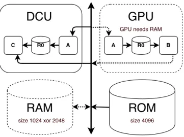
On the hardware side (cf. Fig. 2), the platform provides image pro-cessing capabilities through non programmable pipeline processors of DCU (Display Controller Unit) or GP U (Graphic Processing Unit)
Figure 1: Functional specification
type, as well as data storage functionalities through RAM (Random Access Memory) and ROM (Read Only Memory). RAM and GP U are optional in the actual hardware products, so a system implemen-tation may contain or not these components. Among variabilities in platforms, one can write data into and/or read data from RAM memory while only reading data is possible from ROM. Moreover, memory storage have limited and possibly variable (e.g. RAM) ca-pacity. Contrary to a DCU, which renders directly processed images into display, a GP U needs to store its processing result into RAM. Graphical hardware processors are often designed as a multi-step pipeline, composed of several hardware implemented processing steps, and processor internal fifo memory buffers transferring data from one step to another. In our example, while a GP U can apply A followed by B processing on images in a single pass, a DCU can applyA, then followed by C.
Figure 2: Platform specification
Images and processing could be, respectively, stored and pro-cessed by multiple components, while images can be stored on RAM or on ROM: taskA could be processed by both GPU and DCU, but a data-flow variant containingB task can only be implemented on a system containing a GP U. Finally, data mapping on memory are constrained in terms of storage capacity.
Assessing the Functional Feasibility of Variability-Intensive Data Flow-Oriented Systems SAC 2018, April 9–13, 2018, Pau, France
Consequently, to be valid, a system implementation has to fulfill (i) structural constraints such as not violating maximum memory capacities, (ii) behavioral constraints such as using correctly pro-cessor pipelines and memories, and (iii) variability constraints such as component dependency and exclusion. In our example, the ap-plication data-flow has 4 variants while the Platform exposes 3 architecture variants. Even with this simplified case, this leads to 178 possible implementations, in which 58 satisfy constraints and could be developed by engineers.1
2.3
Related Work
In the context of our work, engineers must be assisted to assess the functional feasibility of the different potential embedded system solutions, with means to capture both the high-level functional requirements and the specifications of targeted variable platforms. Ideally, a solution should be able to capture structural, behavioral and variability properties of both functional and platform speci-fications at a fine-grained level, so to use these input models to automatically infer all possible embedded system implementation designs and assess the resulting consistent design space.
In the software product line engineering, lots of approaches[1, 9] are capable to model variable transition-based systems such as safety-critical systems or protocols, and to validate, through variability-aware model-checking, temporal properties and behav-ioral aspects. However, given high-level data-flows and platform specifications, these approaches are not capable of automatically map data-flows on platforms in order to infer and assess the re-sulting design space. Assessing the different mapping manually is not feasible in practice, as the activity would be tedious and error-prone.
In embedded system design engineering, most of the approaches capture high-level application and platform specifications, and map an application on hardware platforms in order to find, bydesign space exploration, an optimized system implementation for a single functional specification on a single platform [15, 23]. Consequently, they do not capture nor manage variability at the application level and hardware platform variability is limited to component capaci-ties (e.g. memory and bus size, processor frequency). Some other approaches try to handle some limited variability in functional specifications (e.g. optional task, alternative tasks, variable data) (as multiple scenarios [20, 25] or multi-modes systems [18, 26]), but they do not manage platform variability. Some others try to handle some limited variability in platforms (e.g. optional resource, resource dependency, memories sizes) with reconfigurable archi-tectures [21, 22][19]). To the best of our knowledge, none of these approaches handle variability in both application and platform sides so to assess the feasibility of our class of problem.
Interestingly, the recent approach of Graf et. al. [13, 14] manages some variability in both platform and functional specifications. On the platform variability side, resource components can be selected or not, while optional and mutually exclusive task groups are man-aged on the functional part. However, the approach is handling a coarse-grain form of requirements and cannot capture some of our
1
Finding the best solution among the remaining correct solutions is also an important problem, but out of the scope of this paper.
specifications (e.g.data and memory sizes, as well as platform as-pects such as processor pipelines or fifo buffers). Additionally, only structural validation of the system implementations is supported. Behavioral properties (e.g. data sizes, memory capacities, graphic pipelines) and behavioral constraints (e.g., absence of deadlock, reachability, liveness, safety etc.), which are fundamental in our case, cannot be checked.
3
PROPOSED FRAMEWORK
3.1
Overview
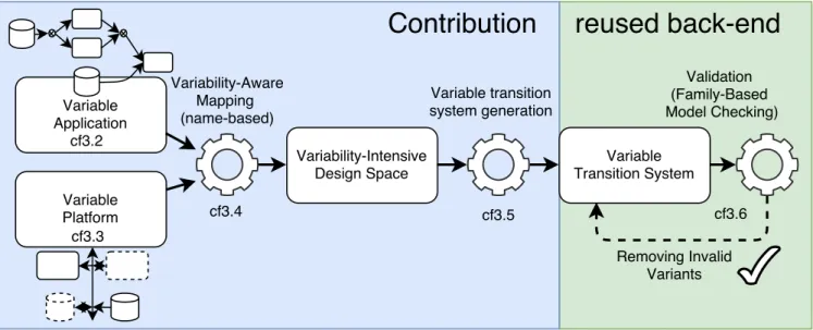
The proposed approach follows a model driven decomposition, based on the well-known robust Y-Chart pattern [2, 16], which separates application and platform into different concerns. This allows modular specification and reasoning about the different parts of the specified embedded systems. Given high-level variable dataflow and platform inputs that notably captures the variability of functional and platform specifications, the framework will i) map all implementation of each data-flow variants on each plat-form configuration, ii) generate a Featured Transition System(FTS) [9] from the system design space model, i.e. representing system implementations (cf. Fig. 3). This model consists in an extended form of automaton product line, which is then iii) checked in one run by a variability-aware model checker.
As shown on Fig. 3, our framework consists of three main models and two processes. We give here an overview while the following sections will detail and illustrate these elements.
Variable applications: a functional expert is in charge of captur-ing the functional requirements (cf.fig. 1) of the embedded system through an extended data-flow (cf. sec. 3.2). This model contains the classic structure and behavior of the data-flow (data, task, data-path, etc.), but also captures the variability in both structural properties (e.g., data size) and behavioral properties (e.g., alternative flows).
Variable platforms: on this side, a platform expert is in charge of expressing the platform specification (cf. fig. 2) as a templated component based system (cf. sec. 3.3). This model contains a set of components connected with each others. Similarly to the appli-cation one, the platform model also captures the variability of the defined components.
Variability-aware mapping process: The mapping algorithm (cf. sec. 3.4) consumes the application and platform input models previ-ously defined and generates theVariability-Intensive Design Space, i.e. representing system implementations. It is made of two steps: (i) it finds for each task data and data-path (cf. fig. 1) all the possible mappings on appropriate platform processors and storage (cf. fig. 2); basically this is done by matching the task names with the names of the hardware functions of processors; data-paths are mapped on reachable memory of appropriate processor hardware functions; (ii) as the design space contains all mapping possibilities, the algo-rithm prunes unfeasible mappings w.r.t. structural and variability constraints.
Design space as a behavioral product line: From the system de-sign space model, aBehavioral Product Line representing all system implementations is generated (cf. sec. 3.5). This product line is rep-resented as a featured automaton, so that we can reuse and adapt techniques that rely on variability-aware model-checking to vali-date the inferred systems. The basic idea is to transform a variable
Figure 3: Framework Overview
data-flow, a variable platform, and mappings to a data-flow automa-ton using, through a mapping automaautoma-ton, a platform automaautoma-ton to execute it. Valid executions of the application automaton should then respect generated properties representing end state reachabil-ity to ensure that the execution is correctly scheduled and executed onto the platform automaton.
Validation process: The validation process reuses automated rea-soning techniques to assess structural and behavioral functional feasibility of the system variants represented by the behavioral product line (cf. sec. 3.6). The model checking is going to determine classic properties, such as safety, absence of deadlock, and our state reachability generated property, on all variants in one run. As a result, the validation solves and extracts valid variants respecting all structural, behavioral and variability constraints.
3.2
Applications as Variable Data-Flows
In our approach, a functional expert captures structure, behavior (data, task, data-path, etc.) and variability aspects (data size, alter-native flows, etc.) of the functional requirements of the embedded system through an extended data-flow model. The extensions con-cern variability and data aspects of functional requirements, and in the following, we propose a formal data-flow model to do so.
Definition 1. A variable data-flow graph is a tuple V DG = (T, D, Path, E, ζ ) where:
•T is a set of tasks,
•D is a set of source data, and, ζ : D → {s0, ..., si ∈ N
∗}returns
a set of alternative sizes of data,
|ζ (d ∈ D)| =
> 1, if d has a variable size 1, ifd has not a variable size
•Path is a set of data-paths by which producer and consumer (i.e. tasks and data) are connected.
•E ⊆ (T ∪ D) × Path × T is the set of edges representing flows processing between producers and consumers.
The set of connected, input data-paths to a taskI (t ), output data-paths from a task or dataO (v) are denoted by:
I (t ) : {p ∈ Path|(x,p, t ) ∈ E},
O (v ∈ T ∪ D) : {p ∈ Path|(v,p, x) ∈ E}.
SimilarlyI (p), input tasks to a output data-paths, and O (p), output tasks from a input data-paths, are denoted by:
I (p) : {prod ∈ T ∪ D|(prod,p, x) ∈ E}, O (p) : {t ∈ T |(x,p, t ) ∈ E}.
|I (p)| + |O(p)| =
> 2, if p has alternative flows 2, ifp has not flow variability
,
A variable data-flow represents multiple data-flow variants. To implicitly represent all these variants in a single model, we follow the same approach as in variable workflows from [13], allowing data-paths to have multiple input and output tasks connected.
A data-path can be connected to multiple alternative, input tasks if|I (p)| > 1, and output tasks if |O (p)| > 1. But, If |I (p)| = 1 ∧ |O (p)| = 1, the data-path is connected to only one input and output task (i.e the data-path has no flow variability).
As data can have alternative sizes, we introduce the functionζ which returns the set of alternative sizesS = ζ (d), each datum has at least one size and if|ζ (d)| > 1 the size of d is variable.
If the data-flow has no flow variability,∀p ∈ Path, |I (p)| + |O (p)| = 2, and no data variability, ∀d ∈ D, |ζ (d)| = 1, the data-flow is not variable.
The functional specification of the case studyV DGuc is then represented as (Tuc= {a,b,c}, Duc= {d1, d2}, Pathuc= {p1, p2, p3}, Euc= {(d1, p1, a), (a,p2, c), (d1, p1,b), (b,p2, c), (d2, p3, c)}) with, ζ (d1)= 512, ζ (d2)= {512, 1024}, I (p1)= d1, I (p2)= {a,b}, I (p3)= d2, O (p1)= {a,b},O(p2)= c,O(p3)= c, I (a) = I (b) = p1, I (c) = {p2, p3},
Assessing the Functional Feasibility of Variability-Intensive Data Flow-Oriented Systems SAC 2018, April 9–13, 2018, Pau, France
3.3
Platforms as Variable Resource Graphs
A variable platform specification is represented by a templated com-ponent based system (multi-pass processors, streaming processor, read-only memory, read-write memory, write-only memory, first-in-first-out buffers etc) where platform can have optional resource components and variability constraints on resources (dependency, incompatibility, etc.). To capture variability aspects of a platform specification, we propose a formal architecture model defined as follows.
Definition 2. A variable resource graph is a tuple V RG = (Proc, S,Cs, ξ , θ, ϕr equir es, ϕexcludes) where:
•Proc = (F, B,Cb⊆(F × B) × (B × F )) is a processor composed of a setF of possible functions, B is a set of processor inter-nal first-in-first-out buffers andCbthe connections between the different functions and buffers representing the processor pipeline.
•S is a set of memory storage, and ξ : S → {c0, ..., ci ∈ N∗}
returns a set of alternative capacities of storage S,
|ξ (s ∈ S)| =
> 1, if s has a variable storage capacity 1, ifs has not a variable storage capacity •Cs ⊆(S × Proc) ∪ (Proc × S) is the set of connections between
memory storage and processors,
•R ⊆ Proc ∪ S is the set of resource components (i.e. processors and memory storage),
•θ : R → B return true if a component (i.e. processor or memory storage) is optional,
•ϕr equir es : R → R captures dependency between resource components, similarlyϕexcludes:R → R captures incompat-ibility.
The set of, input memories to a processor functionI (f ), output mem-ories from a processor functionO (f ) are denoted by:
∃p = (F, B,Cb) ∈Proc,
I (f ∈ F ) : {m ∈ S ∪ B|(m,p) ∈ Cs∨(m, f ) ∈ Cb}, O (f ∈ F ) : {m ∈ S ∪ B|(p,m) ∈ Cs∨(f ,m) ∈ Cb}.
As a variable platform represents multiple platform configura-tions, we also capture implicitly all these configurations by intro-ducing several functions,θ manages the optionality of a resource component. Ifθ (r ) = ⊥ the resource is mandatory, otherwise the resource is optional,ϕr equir esandϕexcludesmanages constrained relations of dependency and incompatibility between resource com-ponents.ϕr equir es(r ) = r0means that ifr is implemented then r0must be implemented too.r depends on r0. On the contrary
ϕexcludes(r ) = r0means thatr and r0cannot be implemented on
the same platform variant.r and r0are alternatives.
As memory storage can have alternative capacities, we introduce the functionξ which returns the set of alternative capacities C = ξ (s), each memory storage has at least one size and if |ξ (s)| > 1 the capacity ofs is variable.
If the platform has no component variability∀r ∈ R, θ (r ) = ⊥ and no variable memory storage,∀s ∈ S, |ξ (s)| = 1, the platform is not variable.
The platform specification of the case studyVGucis then for-malized as
(Procuc= {DCU ,GPU }, Suc= {RAM, ROM},
Csuc = {(RAM, DCU ), (ROM, DCU ),
(RAM,GPU ), (ROM,GPU ), (GPU , RAM)}) where,
DCU = (Fdcu = {adcu, cdcu}, Bdcu = r0dcu,
Cbdcu = {(adcu, r0dcu), (r0dcu, cdcu)}), GPU = (Fдpu= {aдpu,bдpu}, Bдpu= r0дpu,
Cbдpu{(aдpu, r0дpu), (r0дpu,bдpu)}), with,
ξ (ROM) = 4096, ξ (RAM) = {1024, 2048}, θ (GPU ) = θ (RAM) = ⊤,θ (DCU ) = θ (ROM) = ⊥ ϕr equir es(GPU ) = RAM, ϕr equir es(RAM) = ∅, I (aдpu)= {ROM, RAM},O(aдpu)= {r0дpu, RAM},
I (cdcu)= {r0dcu, ROM, RAM}, O (cdcu)= ∅.
3.4
Variability-Aware Mapping Process
The mapping algorithm takes as inputs the variable data-flow and configurable platform models in order to find all embedded system implementations. We propose a mapping model to not only capture all implementations of a single data-flow into a single platform but to capture all data-flow variants implementations onto all platform configurations. Our variability-aware mapping model can be seen as a product line of traditional mapping models.
Definition 3. A variability-aware data-flow-oriented mapping V M = (Tm, Dm, Em) where:
•Tm ⊆ T ×F is the set of possible mappings of tasks on processors ∀(t, f ) ∈ Tm, t can be mapped on processor function f because
f can implement t,
•Dm ⊆ D × S is the set of mappings of data on memory storage, •Em ⊆ E × (S ∪ B) is the set of data-paths mapping on memory
by which data are consumed/produced.
Definition 4. The Variability-Aware Mapping functionM = V DG × V RG → V M sorts topologically the data-flow and finds appropriate mapping for each data, task and paths of the data-flow using resources of the resource graph.
Basically, each valid mapping should respect some constraints such as that
(1) All tasks are mapped to, a least, one processor function: ∀t ∈ T , ∃(t, f ) ∈ Tm,
(2) All data are mapped to, at least, one memory storage: ∀d ∈ D, ∃(d, s) ∈ Dm,
(3) All data-paths are mapped to, at least, one appropriate mapping. For data-path starting by an input datum, the storage on which the datum is mapped has to be reachable by the processor function on which the task consuming the datum is mapped.
∀e = (d ∈ D,p, t) ∈ E, ∃(e,s ∈ S) ∈ Em, ∃(d, s) ∈ Dm, ∃(t, f ) ∈ Tm, s ∈ I (f ),
For data-path between tasks, the memory on which the output of the first task is mapped has to be reachable by the processor function on which the second task is mapped.
∀e = (t ∈ T,p, t′) ∈E, ∃(e,m) ∈ Em,
∃(t, f ) ∈ Tm, ∃(t′, f′) ∈Tm,m ∈ O (f ) ∧ m ∈ I (f′)
The mapping model of the case studyV Mucis then formalized as (Tmuc= {(a, adcu), (a, aдpu), (b,bдpu), (c, cdcu)},
Emuc= {((d1, p1, a), RAM), ((d1, p1, a), ROM),
((d1, p1,b), RAM), ((d1, p1,b), ROM),
((a,p2, c), r0dcu), ((a,p2, c), RAM), ((b,p2, c), RAM),
((d2, p3, c), RAM), ((d2, p3, ROM))})
Finally, The design space representing all system implementa-tions, calledvariability-intensive embedded system design space is then composed of a data-flow, platform and mapping:
V DS ⊆ (V DG × V RG × V M).
3.5
Design Space as a Behavioral Product Line
Automata and model-checking techniques have been widely used to model and validate real-time and embedded systems [4, 5]. In-terestingly, the basic approach used is to schedule an application automaton using a platform automaton [11]. Unfortunately, these approaches are not design to manage any variability aspect of spec-ifications.
Our framework relies on Featured-Transition-Systems (FTS) to represent and validate the design space. FTS has the strength to model explicitly the variability points structurally, through a Fea-ture Diagram[3](FD), instead of modeling variability points behav-iorally, by optional transition with possible constraints[24]. This eases the transformation to featured automaton and the removal of invalid implementations from it. In our approach, we also use LT L property to ensure that all valid execution paths of all system implementations reach the end state of all task of the data-flow.
Definition 5. A featured automaton is a tupleFA =
(Loc, Loc0, I, Act ⊆ Af f ∪ϕ ∪Com, trans, χ,Ch, L, AP,d, λ) such
that:
•Loc is a finite set of locations, Loc0 ∈ Loc, is a set of initial
states andI ∈ Loc, is a set of final states, •Ch is a finite set of communication channels, • χ is a finite set of variables,
•Act is a set of, Af f which is a finite set of variable affectations, ϕ which is a finite set of guards in a boolean expression form andCom ⊆ {c!m, c?m, c!?m|c ∈ Ch,m ∈ χ }, which is a set of communications,
•trans ⊆ Loc × Act × Loc are state transitions,
•d = (N ⊆ Nm∪Nopt∪Nxor, DE ⊆ N × N ,Tcl) is a Feature Diagram (FD),N is the set of mandatory, optional and alter-natives features,DE represents relation between features, Tcl are constraints between features,Jd KF D ⊆ P(N ) is the set of valid product configurations,
•λ : trans → B(N ) is a total function that labels transitions with feature expressions.
•AP is a set of atomic proposition and L : Loc → AP labels transitions with atomic propositions.
A transitions−→α s′is possible for the set of product configurations P ⊆Jλ (s
α
−→s′)K and if ∀д ∈ α ∩ ϕ, д is satisfied,
∀(c?m) ∈ α ∩ Com, wait for data event c!m,
∀(c!?m0) ∈α ∩Com, send data event c!m0but wait for data event
c!m1withm0= m1.
Definition 6. A Linear Temporal Logic property (LT L) is a tem-poral expression of atomic proposition that all possible executions of system variants should satisfy as,J f aKF A|= φ where
φ ::= a ∈ AP |φ ∧ φ| ⋄ φ . Symbol ⋄ means that the property will become true at some point in the future.
We now show how our design space is transformed to aFA. To simplify the transformation process, let us use the following functions:
f : T ∪ Path ∪ R → N , fs :D ∪ S × N∗→N , fto:Path → N , ff rom:Path → N ,
fto:Path × T → N , ff rom:T ∪ D × Path → N ,
fm :T ∪ Path → N , ftm:T × F → N , fpm:Path × S ∪ B → N , which transforms model elements to features.
For example, in our case study, the functions would be: f (a) = A, fs(d2, 1024) = D2Size1024
fto(p1)= p1_To, ff rom(pf rom)= p1_From,
fto(p1, a) = P1ToA, ff rom(a,p2)= P2FromA,
fm(a) = Am, fm(p1)= P1m,
ftm(a, adcu)= AOnAdcu, fpm(p1, ROM) = p1OnROM
f (RAM) = RAM, fs(RAM, 1024) = RAMSize1024, ...
Similarly,
c : T ∪ D ∪ Path ∪ F ∪ S → Ch, cm:T ∪ Path → Ch
transforms model elements to communication channels to inter-act with them at automaton level.
A first functionGenF A:V DG → FA×LT L transforms a variable data-flow graph into aFA and generates the LT L property in the following way.
(1.1) it transforms each datumd with variable size into a xor feature group (Cf. fig.4(a)):
ζ (d) > 1 =⇒ ∀s ∈ ζ (d), ∃(f (d) ∈ Nxor, fs(d, s)) ∈ DE
(1.2) it creates the automaton for each source datumd (Cf.fig.4(b)), after setting the datum size, calling the mapping automaton (Cf. fig. 6(a, b)) that will allocate the datum on the memory. ∀s ∈ ζ (d), ∃{t0= (s0 size (in)=s −−−−−−−−−→s1) , where, |ζ (d)| > 1 =⇒ λ(t0)= fs(d, s), s1 ∀p ∈O (d ),cm(p)!?in −−−−−−−−−−−−−−−−−→s2, s2 ∀p ∈O (d ),c (p)!in −−−−−−−−−−−−−−−→s3} ∈trans
(2.1) it transforms each variable data-pathp in a xor feature group (Cf. fig. 4(a)).
|O (p)| > 1 =⇒ ∀o ∈ O(p), ∃(fto(p) ∈ Nxor, fto(p, o)) ∈ DE |I (p)| > 1 =⇒ ∀i ∈ I (p),
∃(ff rom(p) ∈ Nxor, ff rom(i,p)) ∈ DE
(3.1) it creates task/data-paths consistency constraints (Cf. fig. 4(a)).
∀t ∈ T , ∀p ∈ |I (t )|, |O (p)| > 1 =⇒ ∃(f (t ) ⇐⇒ fto(p, t )) ∈ Tcl
∀t ∈ T , ∀p ∈ |O (t )|, |I (p)| > 1, ∃(f (t ) ⇐⇒ ff rom(t,p)) ∈ Tcl
(3.2) it creates for each taskt the automaton (Cf. fig. 4(c)) that will wait for data-paths allocation, then call the mapping automaton (Cf. fig. 6(c)) to execute the task.
∃{t0= (s0 ∀p ∈I (t ),c (p)?in −−−−−−−−−−−−−−→s1), where, f (t ) ∈ Nopt =⇒ λ(t0)= f (t) ∧ λ((s0→−s4) ∈trans) = ¬f (t), s1 ∀p ∈O (t ),cm(p)!?out −−−−−−−−−−−−−−−−−−→s2, s2 cm(t )!?in,out −−−−−−−−−−−−→s3,
Assessing the Functional Feasibility of Variability-Intensive Data Flow-Oriented Systems SAC 2018, April 9–13, 2018, Pau, France
s3
∀p ∈O (t ),c (p)!out
−−−−−−−−−−−−−−−→s4∈I,
where,L(s4)= tend ∈AP } ∈ trans
(3.3) it generates theLT L formula that checks that a valid execu-tion must, at some point, satisfy atomic proposiexecu-tion of all data-flow task terminal states.
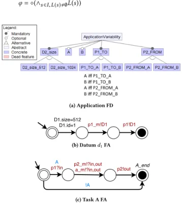
φ = ⋄(∧s ∈I,L(s ),∅L(s))
(a) Application FD
(b) Datumd1FA
(c) Task A FA
Figure 4: Partial variable data-flow application FA
The second functionGenF A:V RG → FA transforms a variable resource graph into aFA in the following way.
(1) it creates feature constraints on resource implementation (Cf. fig. 5(a)).
∀r ∈ R, θ (r ) = ⊤ =⇒ ∃f (r ) ∈ Nopt
∀r ∈ R, ∀rr eq ∈ϕr equir es(r ), ∃(f (r ) =⇒ f (rr eq)) ∈Tcl ∀r ∈ R, ∀rexc ∈ ϕexcludes(r ), ∃(f (r ) =⇒ ¬f (rexc)) ∈ Tcl
(2.1) it creates for each storages features representing storage alternative sizes.
∀c ∈ ξ (s), ∃(f (s) ∈ Nxor, fs(s, c)) ∈ DE
(2.2) it creates for each storages an automaton that represents basic memory behavior (Cf. fig. 5(b)),cons and cap are re-spectively the consumed size and the maximal capacity of the storage. Through channels, one can allocate memory, and if there is not enough memory, an error is raised. ∀c ∈ ξ (s), ∃{t0= (s0 cons=0 −−−−−−→s1), where, f (s) ∈ Nopt =⇒ λ(t0)= f (s) ∧ λ((s0→−s4) ∈trans) = ¬f (s), s1 cap=c −−−−−−→s2, where,λ(s1 cap=c −−−−−−→s2)= f (s,c), s2 c (s )?in,cons+=size (in) −−−−−−−−−−−−−−−−−−−−−→s3, s3 cons <size −−−−−−−−−−→s2, s3
cons ≥size,er ror
−−−−−−−−−−−−−−−→s4} ∈trans
(3) it creates for each processorp an automaton that models basic graphic processor pipeline behavior (cf. fig. 5(c)). When a processor function is executed, the input and output are checked to verify that the pipeline is not misused.
∀p = (F, B,Cb) ∈Proc, ∀f ∈ F, ∀(si, p) ∈ Cs, ∀(p, so) ∈Ws, ∀(bi, f ) ∈ Cb, ∀(f ,bo) ∈Cb, ∃{t0= (s0 c (f )?in,out −−−−−−−−−−→s1), where, f (p) ∈ Nopt =⇒ λ(t0)= f (p) ∧ λ((s0→−s4) ∈trans) = ¬f (p), s1
loc (in)=si∧∀(bi,f ) ∈Rb,bi=f ree
−−−−−−−−−−−−−−−−−−−−−−−−−−−−→s2,
s1
loc (in)=bi∧bi=in
−−−−−−−−−−−−−−−−→s2,
s2
loc (out )=so∧∀(f ,bo) ∈Wb,bo=f ree
−−−−−−−−−−−−−−−−−−−−−−−−−−−−−−−→s3,
s2
loc (out )=bo∧bo=f ree
−−−−−−−−−−−−−−−−−−−−→s3, s3
c (f )!in,out
−−−−−−−−−−→s0} ∈trans
A third functionGenF A:V M → FA transforms a variability-aware dataflow-oriented mapping into aFA as follows.
(1.1) it creates features representing all possible task mappings on processor function (cf. fig. 6(a)).
∀(t, f ) ∈ Tm, ∃(fm(t ) ∈ Nxor, ftm(t, f )) ∈ DE
(1.2) it creates for each task mapping the automaton that executes the processor function according to the mapping configura-tion (cf. fig. 6(c)). ∀t ∈ T , ∀(t, f ) ∈ Tm, ∃{t0= (s0 cm(t )?in,out −−−−−−−−−−−−→s1), where, fm(t ) ∈ Nopt =⇒ λ(t0)= fm(t ) ∧ λ((s0→−s3) ∈trans) = ¬fm(t ) t1= (s1 c (f )!?in,out −−−−−−−−−−−→s2), where,λ(t1)= ftm(t, f ), s2 cm(t )!in,out −−−−−−−−−−−→s3}, ∈ trans
(2.1) Like 1.1, it creates features representing all possible data-path mappings on memory.
∀((x,p,y), s) ∈ Em, ∃(fm(p) ∈ Nxor, fpm(p, s)) ∈ DE
(2.2) Like 2.2, it creates for each data-path mapping the automaton that allocates memory (Cf. fig.6(b)).
∀p ∈ Path, ∀((x,p,y), s) ∈ Em, ∃{s0 cm(p)?out −−−−−−−−−→ s1, t0 = (s1 c (s )!?out,loc (d )=s −−−−−−−−−−−−−−−−→s2), where, λ(t0)= fpm(p, s), s2 cm(p)!out −−−−−−−−−→s3} ∈trans
Finally the functionGenF A:V DS → FA, defined by: GenF A((vdд,vrд,vm)) :
GenF A(vdд)||GenF A(vrд)||GenF A(vm),
transforms our design space into a featured automaton.
To preserve the consistency of the design space, variability con-straints are inferred such as:
(1.1) Task features with variable data-path features are not im-plemented on all data-flow variants, then those features are made optional (Cf. fig. 4(a)).
∀t ∈ T ,
∃pi ∈I (t ), |O (pi)| > 1 ∨ ∃po ∈O (t ), |I (po)| > 1 =⇒ f (t) ∈ Nopt
(1.2) Variable task features have their mapping variable too; if a task feature is implemented its mapping must be imple-mented too, and vice-versa (Cf. fig. 4(a) & 6(a)).
∀t ∈ T , f (t ) ∈ Nopt =⇒
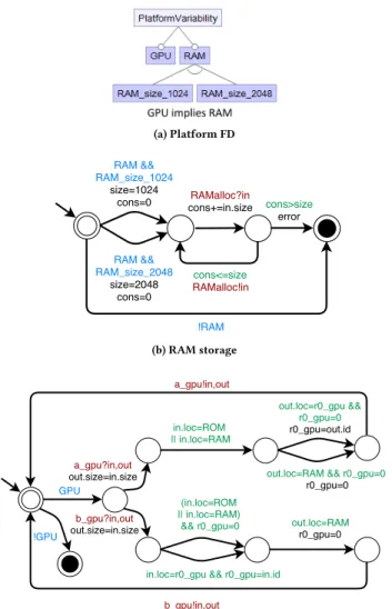
(a) Platform FD
(b) RAM storage
(c) GPU processor
Figure 5: Partial variable platform FA
(2.1) If a task mapping feature is implemented on a processor function, the implemented input and output path mappings have to be reachable (Cf. fig. 6(a)).
∀(t, f ) ∈ Tm, ∀pi ∈I (t ), ∀po ∈O (t ), ∃(ftm(t, f ) ⇐⇒ ( W ((x,pi,t ),m ∈I (f )) ∈Em fpm(pi,m))∧ ( W ((t,po,x ),m′∈O (f )) ∈Em fpm(po,m′))) ∈Tcl
(3.1) If a task mapping feature using an optional processor is implemented, the processor must be implemented too. ∀p = (F, x,y) ∈ Proc, f (p) ∈ Nopt, ∀(t, f ∈ F ) ∈ Tm
=⇒ ∃(ftm(t, f ) =⇒ f (p)) ∈ Tcl
Similarly, if a data-path mapping feature is implemented on fifo buffer of optional processor (3.2) or optional memory storage (3.3), the resource have to be implemented.
(3.2) ∀pu = (F, B, x) ∈ Proc, ∀((y,p, z),b ∈ B) ∈ Em, f (pu) ∈ Nopt =⇒ ∃(fpm(p,b) =⇒ f (pu)) ∈ Tcl
(3.3) ∀((x,p,y), s ∈ S) ∈ Em, f (s) ∈ Nopt =⇒ ∃(fpm(p, s) =⇒ f (s)) ∈ Tcl
As an illustration, in our case study, the rules would be: (1.2)A ⇐⇒ Am,B ⇐⇒ Bm
(3.1)BOnBдpu =⇒ GPU , AOnAдpu =⇒ GPU (3.2)P2OnR0дpu =⇒ GPU
(3.3)P1OnRAM =⇒ RAM, P2OnRAM =⇒ RAM P3OnRam =⇒ RAM
(a) Mapping FD
(b) data-path Mappingp1FA
(c) Task Mapping A FA
Figure 6: Partial Variability-Aware Mapping FA
3.6
Validation Process
As our form of behavioral product lines is based on FTS [9], model checking techniques can be directly reused. In our implementation (Cf. next section), we reuse the ProVeLines/SNIP checker as a back-end for the validation process. The process consists in verifying all execution paths of all products
J f aKF Aof the product line, in an efficient way by exploiting commonalities between different products. Theoretically, the more the products share common be-havior and the more efficient should be the variability aware model checking in comparison of iterative model checking on individual systems [8]. Instead of exploring all executions for each system implementation, the model-checker explores an executionπ once for all implementationsP able to produce this specific execution:
Assessing the Functional Feasibility of Variability-Intensive Data Flow-Oriented Systems SAC 2018, April 9–13, 2018, Pau, France
As mentioned in the previous section, some system configura-tions may expose inconsistent behaviors (e.g., memory allocation error, violation of graphical pipeline constraints). These behaviors will abort the execution and the basic properties (e.g. safety, absence of deadlock, state reachability) will obviously not be satisfied. In our validation process, we are able to remove these configurations from the system by relying again on the back-end model checker [8]. It computes the set of bad product configurations, which we re-move from the feature diagram of the product line by adding the appropriate cross-tree constraints.
4
EVALUATION
4.1
Implementation
The presented framework has been entirely implemented. The vari-able application and platform input meta-models, the mapping algo-rithm and the removal of invalid variants from the variable design space are implemented in Java. Functional and platform variability specifications are entered through a dedicated API, and the frame-work then generates explicit variability models. The frameframe-work implementation also infers knowledge about task implementation capabilities of processors, and generates task, data-path, processor and memory automata by automatically configuring predefined templates.
The mapping algorithm implementation is traversing all model representations to find the appropriate mappings by name match-ing. Then it generates constrained Feature Models and Featured Automata in TVL [6] and fPromela specifications. Automated rea-soning techniques can be used over TVL Feature Models (e.g. SAT solving [17]) to reason about the structural variability of the rep-resented system. As for the validation process of the behavioral product line, it uses the ProVeLines/SNIP model-checker [7, 10], which takes TVL and fPromela files as input.
4.2
Industrial Use Case
In order to validate our tooled approach on an industrial scale, we applied it to a real low-end market instrument cluster provided by Visteon, the automotive systems company we collaborate with.
The functional requirements of the cluster represents a variable data-flow with 3 source images processed by 8 tasks connected by 9 data-paths. Each source image has two different resolutions (i.e HD and LD) and two tasks sub flow sequences are alternative through axor join/split data-path, resulting in 16 data-flow variants. The platform specification of the cluster is then represented by a variable hardware component system with 2 memories (a Video RAM and a ROM Flash) and 3 processors (two multi-pass GP U bitblitter and one streaming- based DCU). Each processor has a pipeline processing of 4 stages and 3 fifo buffers. In terms of platform variability, the 2 bitblitters and the VRAM are optional. Each memory has 2 different configurable sizes at manufacturing time. The number of platform configurations in the use case is then 24.
If each data-flow variant had one possible implementation on each platform configuration, the number of different cluster system implementations would be 384. In reality, some platform configura-tions do not provide the graphical functionalities required by some data-flow variants. Furthermore, due to multiple task implemen-tation choices, data-flow variants have several thousand possible
implementation alternatives onto a platform configuration. Setting the platform configuration to the higher end (i.e. selecting VRAM and all processors), one can find 72 and 78 possible implementa-tions for two data-flow variants that take different xor data-path decisions. This is due to more pipelining opportunities in the sec-ond data-flow variant, even if there is more data-path mapping possibilities in the first one.
Table 1 shows time measurements of the complete toolchain while varying the different variability dimensions over the use case. In the first seven rows, we observe that the whole process is performing well with small to medium scale of variabilities. Data and memory size variability verifications are faster and require more state exploration than platform component and data-path variabilities. Component and data-path variabilities are also slower to check than data and memory size variabilities. It is likely to be due to the fact that contrary to size variability, hardware component and data-path variability are strongly impacting the implementation variability, and consequently the state space of the model checker.
We also have complemented this experimentation by taking a single structural data-flow from the industrial use case with a simulated larger platforms with multiple memories and processors. Results in the last three rows of Table 1 show that the solving can scale to a large number of implementation variants, even if the solving time is significant.
5
CONCLUSION
A tremendous amount of variability can be observed in embedded systems, and especially in data-flow oriented ones, which are now systematically built from highly variable specifications and target diverse hardware platforms configurable at a very high level of detail. To handle the early functional assessment of all these possi-ble configurations, we proposed in this paper a tooled framework that takes variable data-flow specifications and variable hardware platform models to map them together and transform them into a behavioral product line representing the potential design space. The framework allows to use automated reasoning techniques to explore and assess the feasibility of all represented variants in a sin-gle run, and invalid products can be removed by adding constraints to the product line. We also reported on the application of the pro-posed approach to a real-world industrial use case of automotive instrument cluster, showing its potential good applicability.
As future work, we first plan to facilitate the usage of the frame-work with domain specific languages for input models (specifica-tion and platform), and to conduct larger experiments with them. We will also extend the framework by providing guidance when conducting functional validation, and by taking into account non-functional properties (e.g. cost) so to provide optimized product selection as a complement to the functional validation presented in this paper.
6
ACKNOWLEDGMENTS
We thank Visteon Electronics and ANRT for continuously sup-porting this research, especially, Emmanuel Roncoroni and Olivier Bantiche who brought industrial knowledge and expertise in in-strument cluster engineering.
Variability Implementation Platform data-flow States explored Time ms / states / variants variants variants (re-explored) (ms) variants variants
NONE 78 0 0 2453 (331) 27 0.346 31.448
Data size 624 0 8 15254 (2406) 201 0.322 35.976 Platform 424 24 0 5673 (546) 65 0.153 13.379 Platform and data size 3392 24 8 37435 (4856) 602 0.177 11.036 data-path 150 0 2 4727 (981) 74 0.493 31.513 data-path and data size 1200 0 16 29066 (6994) 587 0,489 24,222
ALL >4800 24 16 72704 (14652) 2361 - -Platform mult. mem 16408 40 0 134941 (4534) 4010 0.244 8.224
Platform mult. proc 2848 80 0 19625 (3224) 337 0.118 6.890 Pltf. mult. proc & mem 516608 160 0 1341999 (175304) 289721 0.560 2.597
Table 1: Industrial use case results
REFERENCES
[1] Patrizia Asirelli, Maurice H ter Beek, Stefania Gnesi, and Alessandro Fantechi. 2011. Formal description of variability in product families. InSoftware Product Line Conference (SPLC), 2011 15th International. IEEE, 130–139.
[2] Felice Balarin. 1997.Hardware-software co-design of embedded systems: the POLIS approach. Springer Science & Business Media.
[3] Don Batory. 2005.Feature models, grammars, and propositional formulas. In SPLC, Vol. 3714. Springer, 7–20.
[4] Johan Bengtsson, Kim Larsen, Fredrik Larsson, Paul Pettersson, and Wang Yi. 1996. UPPAAL-a tool suite for automatic verification of real-time systems.Hybrid Systems III (1996), 232–243.
[5] Edmund M Clarke, Orna Grumberg, and Doron Peled. 1999.Model checking. MIT press.
[6] Andreas Classen, Quentin Boucher, and Patrick Heymans. 2011. A text-based approach to feature modelling: Syntax and semantics of TVL.Science of Computer Programming 76, 12 (2011), 1130–1143.
[7] Andreas Classen, Maxime Cordy, Patrick Heymans, Axel Legay, and Pierre-Yves Schobbens. 2012. Model checking software product lines with SNIP.Int. Journal on Software Tools for Technology Transfer (STTT) (2012), 1–24.
[8] Andreas Classen, Patrick Heymans, Pierre-Yves Schobbens, and Axel Legay. 2011. Symbolic model checking of software product lines. InProceedings of the 33rd International Conference on Software Engineering. ACM, 321–330.
[9] Andreas Classen, Patrick Heymans, Pierre-Yves Schobbens, Axel Legay, and Jean-François Raskin. 2010. Model checking lots of systems: efficient verification of temporal properties in software product lines. InProceedings of the 32nd ACM/IEEE International Conference on Software Engineering-Volume 1. ACM, 335– 344.
[10] Maxime Cordy, Andreas Classen, Patrick Heymans, Pierre-Yves Schobbens, and Axel Legay. 2013. ProVeLines: a product line of verifiers for software product lines. InProceedings of the 17th International Software Product Line Conference co-located workshops. ACM, 141–146.
[11] Andreas E Dalsgaard, Mads Chr Olesen, Martin Toft, René Rydhof Hansen, and Kim Guldstrand Larsen. 2010. Metamoc: Modular execution time analysis using model checking. InOASIcs-OpenAccess Series in Informatics, Vol. 15. Schloss Dagstuhl-Leibniz-Zentrum fuer Informatik.
[12] Sebastian Graf, Michael Glaß, Jurgen Teich, and Christoph Lauer. 2014. Multi-variant-based design space exploration for automotive embedded systems. In Design, Automation and Test in Europe Conference and Exhibition (DATE), 2014. IEEE, 1–6.
[13] Sebastian Graf, Michael Glaß, Dominic Wintermann, Jurgen Teich, and Christoph Lauer. 2013. IVaM: Implicit variant modeling and management for automotive embedded systems. InHardware/Software Codesign and System Synthesis (CODES+ ISSS), 2013 International Conference on. IEEE, 1–10.
[14] Sebastian Graf, Sebastian Reinhart, Michael Glaß, Jurgen Teich, and Daniel Platte. 2015. Robust design of E/E architecture component platforms. In52nd Design
Automation Conference (DAC). IEEE, 1–6.
[15] Matthias Gries. 2004. Methods for evaluating and covering the design space during early design development. Integration, the VLSI journal 38, 2 (2004), 131–183.
[16] Bart Kienhuis, Ed Deprettere, Kees Vissers, and Pieter Van Der Wolf. 1997. An approach for quantitative analysis of application-specific dataflow architectures. InApplication-Specific Systems, Architectures and Processors, 1997. Proceedings., IEEE International Conference on. IEEE, 338–349.
[17] Marcilio Mendonca, Andrzej Wasowski, and Krzysztof Czarnecki. 2009. SAT-based analysis of feature models is easy. InProceedings of the 13th International Software Product Line Conference. Carnegie Mellon University, 231–240. [18] Gianluca Palermo, Cristina Silvano, and Vittorio Zaccaria. 2008. Robust
optimiza-tion of SoC architectures: A multi-scenario approach. InEmbedded Systems for Real-Time Multimedia, 2008. ESTImedia 2008. IEEE/ACM/IFIP Workshop on. IEEE, 7–12.
[19] Gianluca Palermo, Cristina Silvano, and Vittorio Zaccaria. 2009. Variability-aware robust design space exploration of chip multiprocessor architectures. InDesign Automation Conference, ASP-DAC. Asia and South Pacific. IEEE, 323–328. [20] Lars Schor, Iuliana Bacivarov, Devendra Rai, Hoeseok Yang, Shin-Haeng Kang,
and Lothar Thiele. 2012. Scenario-based design flow for mapping streaming appli-cations onto on-chip many-core systems. InProceedings of the 2012 international conference on Compilers, architectures and synthesis for embedded systems. ACM, 71–80.
[21] Kamana Sigdel, Mark Thompson, Andy D Pimentel, Carlo Galuzzi, and Koen Bertels. 2009. System-level runtime mapping exploration of reconfigurable archi-tectures. InParallel & Distributed Processing, 2009. IPDPS 2009. IEEE International Symposium on. IEEE, 1–8.
[22] Vlad-Mihai Sima and Koen Bertels. 2009. Runtime decision of hardware or software execution on a heterogeneous reconfigurable platform. InParallel & Distributed Processing, 2009. IPDPS 2009. IEEE International Symposium on. IEEE, 1–6.
[23] Amit Kumar Singh, Muhammad Shafique, Akash Kumar, and Jörg Henkel. 2013. Mapping on multi/many-core systems: survey of current and emerging trends. InProceedings of the 50th Annual Design Automation Conference. ACM, 1. [24] Maurice H ter Beek, Alessandro Fantechi, Stefania Gnesi, and Franco Mazzanti.
2016. Modelling and analysing variability in product families: model checking of modal transition systems with variability constraints.Journal of Logical and Algebraic Methods in Programming 85, 2 (2016), 287–315.
[25] Peter Van Stralen and Andy Pimentel. 2010. Scenario-based design space explo-ration of MPSoCs. InComputer Design (ICCD), 2010 IEEE International Conference on. IEEE, 305–312.
[26] Stefan Wildermann, Felix Reimann, Jürgen Teich, and Zoran Salcic. 2011. Opera-tional mode exploration for reconfigurable systems with multiple applications. InField-Programmable Technology (FPT), 2011 International Conference on. IEEE, 1–8.