HAL Id: hal-02619546
https://hal.archives-ouvertes.fr/hal-02619546
Preprint submitted on 25 May 2020
HAL is a multi-disciplinary open access archive for the deposit and dissemination of sci-entific research documents, whether they are pub-lished or not. The documents may come from teaching and research institutions in France or abroad, or from public or private research centers.
L’archive ouverte pluridisciplinaire HAL, est destinée au dépôt et à la diffusion de documents scientifiques de niveau recherche, publiés ou non, émanant des établissements d’enseignement et de recherche français ou étrangers, des laboratoires publics ou privés.
the COVID-19 dynamics in France
Mircea Sofonea, Bastien Reyné, Baptiste Elie, Ramsès Djidjou-Demasse,
Christian Selinger, Yannis Michalakis, Samuel Alizon
To cite this version:
Mircea Sofonea, Bastien Reyné, Baptiste Elie, Ramsès Djidjou-Demasse, Christian Selinger, et al.. Epidemiological monitoring and control perspectives: application of a parsimonious modelling frame-work to the COVID-19 dynamics in France. 2020. �hal-02619546�
Epidemiological monitoring and control
perspectives: application of a
parsimonious modelling framework to
the COVID-19 dynamics in France
Mircea T. Sofonea
∗, Bastien Reyné, Baptiste Elie, Ramsès Djidjou-Demasse,
5
Christian Selinger, Yannis Michalakis, Samuel Alizon
MIVEGEC (Univ. Montpellier, CNRS 5290, IRD 224) – 911 av. Agropolis BP 64501, 34394 Montpellier Cedex 5, France
∗corresponding author (mircea.sofonea@umontpellier.fr)
Abstract
10
SARS-Cov-2 virus has spread over the world creating one of the fastest pandemics ever. The absence of immunity, asymptomatic transmission, and the relatively high level of virulence of the COVID-19 infection it causes led to a massive flow of patients in intensive care units (ICU). This unprecedented situation calls for rapid and accurate mathematical models to best inform public health policies. We develop an original parsimonious model that accounts for the effect
15
of the age of infection on the natural history of the disease. Analysing the ongoing COVID-19 in France, we estimate the value of the key epidemiological parameters, such as the basic reproduction number (R0), and the efficiency of the national control strategy. We then use our deterministic model to explore several scenarios posterior to lock-down lifting and compare the efficiency of non pharmaceutical interventions (NPI) described in the literature.
20
Keywords: COVID-19, epidemiology, public health, non-pharmaceutical interventions,
1
Introduction
1.1
The COVID-19 pandemic
In Dec 2019, a rapidly increasing number of ‘pneumonia of unknown etiology’ cases in Wuhan,
25
China, triggered a specific surveillance mechanism implemented by China’s Center for Disease Control (CDC) in the wake of the 2003 SARS-CoV pandemic (Li et al., 2020a). In Jan 2020, China CDC identified the new inter-human transmitted pathogen as a coronavirus, which was later named SARS-CoV-2 after its phylogenetically close predecessor (Coronaviridae Study Group of the ICTV,2020). Meanwhile, the respiratory disease for which it is responsible, called
30
COVID-19, was better described from the clinical point of view, especially by identifying age and co-morbidities as risk factors of symptomatic aggravation and fatality (Chen et al.,2020;Huang et al., 2020). Because of its relatively high basic reproduction number (R0≈2.2) in the Wuhan outbreak (Li et al.,2020a) and the high transimissibility of asymptomatic/undocumented cases (Nishiura et al., 2020a; Li et al., 2020b), as well as the intensity of international travel, the
35
virus rapidly spread in mainland China and then all over the world.
On Mar 11, 2020, the WHO announced that the COVID-19 outbreak had reached pandemic stage. To date, no pharmaceutical treatment has proven to be efficient, neither prophylactically nor therapeutically.
1.2
The French situation
40
The documented importation of SARS-CoV-2 on the French metropolitan territory dates back to Jan 24, 2020 with the detection of three cases with a travel history to Wuhan (Stoecklin et al.,2020). These were also the first COVID-19 cases detected in Europe.
From Feb 27, the daily incidence of detected cases started to increase exponentially, followed on Mar 8 by the daily hospital mortality. On Feb 29, the government announced that France
45
had moved to stage 2 of the epidemics with isolated cases, and reminded that masks should only be worn based on medical advice. On Mar 7, the government advocated for basic measures (hand washing, avoiding handshakes) but announced the elections on Mar 15 were not cancelled. On Mar 12, a scientific council was set up and the president announced that from Mar 16, all schools and universities would be closed, before implementing a lock-down for the whole country
from Mar 17. 55 days later, on May 11, the lock-down was lifted.
1.3
COVID-19 epidemic modelling
Mathematical modelling was involved early on to estimate the magnitude of the COVID-19 epidemic in Wuhan. Estimates of the serial interval were obtained rapidly allowing to estimate the basic reproduction number (Li et al.,2020a). Later on, analyses on the number of travelers
55
from Wuhan to Europe and infected by COVID-19 allowed to estimate the magnitude of the epidemics in Wuhan (Imai et al., 2020) or the incubation time of the infection (Backer et al., 2020). Furthermore, stochastic models allowed to better assess the probability to control initial outbreaks (Hellewell et al.,2020). Early models also stressed the importance of detecting infections early on to control the epidemics (Ferretti et al., 2020).
60
It quickly became clear that the epidemic had reached a large enough size to escape stochas-tic forces in Wuhan and that, in spite of a full lock down and travel restrictions, it had spread all over the world, making deterministic models more appropriate. This also led to an increase in modelling efforts because deterministic compartmental models based on ordinary differen-tial equations are more commonly used in epidemiological modelling. However, although these
65
models have useful analytical properties when analysed over a long time period, they are per-form poorly on short time scales. One reason for this is that they are essentially Markovian or ‘memoryless’. This means for instance that an individual that has been infected for 10 days has the same probability to clear the infection that someone infected for less than a day. Over a long time period this effect averages out but on a shorter time scale, even if the dynamics are
70
deterministic, this Markovian assumption makes it difficult to reconcile the model with data. Focusing on the French epidemic,Di Domenico et al. (2020) developed a variant of an SEIR model with multiple levels of infection severity and estimated the R0 to 3.0 (with a 95% CI of 2.8-3.2). Using an SIR model, Magal and Webb (2020) estimated it to 4.5 (no confidence interval computed). Using a meta-population model,Roux et al. (2020) estimated it in various
75
regions of France and found values between 1.7 and 4.2 with a median value of 2.8. Using a simpler SIR model but a more robust statistical framework Roques et al. (2020), found an R0 between 3.1 and 3.3, but also estimated a temporal reproduction number (Rt) after the lock-down of 0.47 (with a 95% CI of 0.45-0.50). Hoertel et al. (2020) developed a detailed
agent-based simulation model with 194 parameters, which allows them to estimate R0 to 3.1
80
(no confidence interval computed) and investigate the effect of different types of interventions on the spread of the epidemics. Finally, Salje et al. (2020), with priority access to restricted ICU patient data, developed a detailed SEIR model with explicit ICU admissions tailored to the French epidemics. Using a detailed statistical inference model, they estimated the R0 to 2.9 (with a 95% CI of 2.8-2.99) and an Rtafter the lock-down of 0.67 (with a 95% CI of 0.65-0.68).
85
The model we introduce is inspired by an earlier optimal control model (Djidjou-Demasse et al.,2020). Taking advantage from its two key qualities, namely being simultaneously determin-istic and tailored for non-exponentially distributed transition times, accurately follow the main properties of COVID-19 epidemic, while limiting the number of compartments and parameters. In this study, by using the French COVID-19 epidemics as an example, we introduce a more
90
mechanistic compartmental model, which explicitly features two categories of critically ill pa-tients. This allows us not only to describe the past state of the epidemic but also to explore the effect of original and ea control strategies.
1.4
A non-markovian discrete-time model
Unlike the majority of deterministic models used in epidemiology (Keeling and Rohani, 2008),
95
ours runs in discrete time, with a time step equal to one day. This choice implies a formalism of numerical sequences that is closer to algorithmic syntax, less compact and less intuitive than that of ordinary differential equations. However, discrete-time models have the great advantage of implementing process memory. Indeed, the usual continuous-time models are said to be memory-less because the probability for an individual to leave a certain compartment,
100
for instance to recover, is independent of the time already spent in this compartment.
The absence of memory does not alter the qualitative properties of the model when an asymptotic behaviour is studied. It can however become extremely oversimplifying when study-ing phenomena over short time scales, that is in the transient regime of the system. Indeed, failing to account for the past may buffer sudden changes in the system. In the case of
COVID-105
19 infections, it is very rare for symptoms to appear the day after contamination. On the contrary, clinical signs appear mostly at the turn of the week following the contamination. Failure to take this into account affects the short-term dynamics and, as we show, make it
impossible to interpret the incidence data.
Although there are ways to correct ordinary differential equation models to deal with each of
110
the above-mentioned situations (e.g. delays, impulses, non-autonomous equations), the discrete-time approach makes it possible to easily accumulate all of these options. It also approaches the very format of the data collected, monitored, and communicated during epidemics on a daily basis.
While accounting for non-Markovian transition times between clinical-epidemiological
com-115
partments, our model remains deterministic. This means that contrarily to agent-based models, it can explore a variety of scenarios in a computationally efficient way. It thus combines the advantages from both stochastic modelling (namely simulating non-exponential-like waiting times) and law of large numbers (namely capturing the general trend of the system by aver-aging). Moreover, the deterministic nature of the model makes it quite parsimonious, allowing
120
unknown parameter values to be estimated, thereby preventing arbitrary choices. Likewise, its simple formulation opens ways to a variety of extensions and facilitates broad applications to health authorities.
1.5
Peak dynamics and epidemic control
By calibrating our model using French data, we show that epidemiological dynamics can be
125
accurately captured. More precisely, we estimate the R0 of the French epidemics to be between 2.59 and 3.39, a number that decreased to between 21.3 and 27.1% of its value after the lock-down (95% likelihood interval).
By comparing our calibrated model to one without memory, we show the importance of allowing model parameters to depend on the age of the infection to accurately capture
short-130
term dynamics. We also investigate the effect of earlier or later implementation of a national lock-down on epidemic peak intensity and timing.
Finally, we use our flexible and statistically robust framework to compare 3 main types of non-pharmaceutical interventions (NPI) that have been proposed in the literature: focusing the control on sub-populations who are more at risk, implementing periodic control, and deploying
135
an adaptive lock-down (also known as ‘stop and go’). We show that these differ in terms of cumulative mortality but also in terms of the cumulative number of people undergoing strict
control. This opens new perspectives for NPI, which are essential until pharmaceutical options become available.
2
Methods
140
2.1
Model structure and dynamics
Following classical epidemiological models (Kermack and McKendrick, 1927; Keeling and Ro-hani, 2008), we group individuals with the same contribution to the dynamics into compart-ments whose densities are tracked over time. We consider age structured dynamics, by splitting each compartment into an arbitrary number of age groups, which are hereafter denoted by an
145
index i. This enhances the model with two key features. First, many COVID-19 clinical pa-rameters are age-dependent, especially the infection fatality rate (Verity et al., 2020a). With this age structure, we can adjust nationwide averages and capture demographic effects by matching demographic data to stratified medical data. Second, we can investigate age-differentiated non-pharmaceutical interventions (NPI). Note that this model can be extended
150
to formally take into account any kind of finer stratification, e.g. age, sex and comorbidities simultaneously. Furtermore, adding a discrete implicit spatial (also known as meta-population) structure is straightforward.
Since hospital admissions and critical cases are less frequent than non-severe infections, we assume that all transmission events occur in the community. A specific extension of the model
155
could be to focus on nosocomial transmission.
The structure of the system is shown in Figure 1. Initially, all individuals in group i belong to the susceptible compartment, the density of which is denoted Si. These individuals can be
infected with a probability Λi called the force of infection (the i subscript indicates that not all
ages are equally susceptible to infection).
160
Upon infection, a fraction 1 − θi of the individuals will develop non critical infections and
move to the Ji,⋅ compartment, where the second subscript indicates the age of the infection (in
days). At each time step, an individual in the compartment Ji,k moves to the compartment Ji,k+1and after g days of infection it moves to the recovered (and assumed lastingly immunized)
compartment Ri.
165
A fraction θi of infections will lead to critical complications (typically acute respiratory
distress syndrome (Bouadma et al., 2020)), and move to the Yi,1 compartment. Every day k,
Figure 1: COVID-19 epidemic discrete time model structure.
Each square represents a group of individuals who share the same clinical kinetics and who contribute equally to the epidemic dynamics. Contiguous squares form a compartment, in which each individual progresses day after day, therefore allowing to capture memory effects of the infection age. Pink boxes correspond to infected individuals in the community (depicted by the yellow area). Light blue boxes represent the hospitalized critical cases (the light blue area depicting the hospital). The purple-grey area corresponds to removed compartments that do not contribute to the epidemic. Arrows between boxes correspond to the daily flow of individuals from one compartment to the other. Dotted arrows depict transitions that occur with probability 1. The i subscript indicates the age group. For the sake of simplicity, only one group is depicted here and only one of the two probabilities is shown for each bifurcating transition (the other being its complementary to 1). Details about the compartments, flows and notations are provided in the main text.
probability 1 − ηk to move to the Yi,k+1 subgroup. No individual of a cohort of critical cases
remains in the Yi,⋅ compartment after h days.
170
As detailed in Appendix S2.5, two groups of hospitalized critical patients are considered. Those who have a substantial chance of recovering and who will benefit from a long stay (at least greater than one day) in an intensive care unit (ICU), are denoted by Hi,⋅. Those who will die,
either after a short stay in ICU or in another ward are denoted by Wi,⋅. Upon hospitalization,
a proportion of the incoming Yi,⋅ moves to Hi,⋅ while the remaining part moves to Wi,⋅. Time
175
to death for the latter compartment is captured by the sequence of υk. For the former, ICU
discharge occurs with probability ρk, k being the number of days after hospitalization, and only
2.2
Forces of infection
In the SIR-like modelling framework, the force of infection refers to the infection rate per
180
capita of susceptibles, often expressed as λ ∶= βI (Keeling and Rohani,2008). Equivalently, the instantaneous incidence is βIS = λS, which is the translation of the mass action law implied by the mean-field approximation made by such spatially unstructured models.
In our discrete time model, the force of infection Λi is not a rate but a daily probability
of infection (per capita of susceptibles from group i) that saturates with the prevalence.
Indi-185
vidual contributions of infected individuals are not additive when prevalence is high because a susceptible host surrounded by infected individuals can be infected by several of them the same day. When prevalence is low, the probability of contamination by multiple infectors the same a day is low and the force of infection is well approximated by the sum of contributions of each infected individual. Λi is therefore a monotonically increasing function of prevalence,
190
bounded by 1 and with a positive initial slope.
As we show in Appendix S2.2, deriving an expression for the force of infection is far from trivial for two reasons. First, we do not have a single class of infected individuals I as in most simple models. We therefore need to define and calculate an effective infectious density at time t (denoted I(t)), which can be seen as the number of individuals in the J and Y classes,
195
weighted by both the level of per-capita contact ratio c (t) and the generation time distribution, here approximated by the serial interval.
As detailed in Appendix S2.2, we find that the force of infection can be written as Λi(t) =
ci(t) I (t)
S0
R0 +ci(t) I (t)
, (1)
where ci denotes the relative contact rate per capita of i-individuals (i.e. the current contact
rate divided by the pre-epidemic baseline), I the effective infectious density, S0 the initial
200
population size and R0 the basic reproduction number. In AppendixS2.2, we also demonstrate the origin of the saturation parameter in the Michaelis-Menten equation, namely S0/R0.
2.3
Data
This model can be applied to any population where COVID-19 incidence data can be collected. However, it also requires additional details, such as the time spent in ICU or the mortality,
205
which is why we apply it to France where at least part of the data is available.
All the model parameters are detailed in Appendix S1. We attempted to calibrate the models to the best of our ability based on the data available at the time of writing this report. For instance, the calculation of µi is based on reports from Santé Publique France. The age
structure of the population is based on the data from the French National Institute of Statistics
210
and Economic Studies (Institut National de la Statistique et des Études Économiques, 2020). Due to the lack of accessible public health data from France, we had to combine it with data from other countries. We therefore approximated the generation time using the serial interval inferred byNishiura et al.(2020a) on transmission pairs from multiple countries, as well as the Infection Fatality Ratio (IFR) computed byVerity et al. (2020a).
215
Further details about the time series data can be found in Appendix S2.4.
2.4
Memory effects
For several key processes in the model, the probability for an event to occur depends on the elapsed time. This is the case for the interval between contamination and hospitalization, through the probability distributions that underlie the ηk sets of parameters. This is motivated
220
by the fact that, as early noticed by clinicians (Bouadma et al.,2020), respiratory complications of COVID-19 arise in a quite narrow time window approximately a week after symptom onset. Memory is also involved in the transmission term. As one can notice, there is no incubation period per se in the model. This is implicitly accounted for in the infectiousness term ζk used
to calculate the force of infection (see Appendix 2.2 for details). Indeed, the compartments
225
that transmit the virus (J and Y ) do so following weights, which we refer to as the discretized generation time, i.e. the daily probability of transmitting the virus each day following the day of infection. Based on empirical data, e.g. the serial interval derived by Nishiura et al.(2020a), the first day these values are very low, then they increase rapidly before decreasing slowly. This modelling approach eventually recovers a classical SIR model for the non-critical cases,
230
additional compartments (such as a latent/exposed E, and convalescent densities) and their corresponding parameters.
We use two parameters to describe non-exponential distribution, which we assume to be Weibull distributions with a shape parameter greater than 1 (which captures the ’ageing’
prop-235
erty) and a scale parameter. Other components of the model could also, in theory, accommodate memory processes, namely the time distribution from hospitalization to ICU discharge or death (ρk and υk). However, preliminary fitting attempts reveal that an exponential (memory-less)
distribution is more parsimonious. In Appendix S2.6, we explain in further details how the distributions for the various waiting times were defined and estimated from the data.
240
For comparison purposes, we also considered the continuous-time memory-less translation of this model (detailed in Appendix S2.9), which proved to be less adequate to capture the dynamics of the French epidemic in France, as shown by Fig.3.
2.5
Parameter estimation and simulation confidence intervals
Parameter estimation is required prior to analyzing the outcome of the model when i) strong
245
simplifying assumptions about the phenomenon under study are made, and ii) some parameter values are not known with sufficient certainty.
First, the strongest assumption of the present model is the mean-field approximation: the population is supposed to be well-mixed, which is obviously not the case at the country scale. Nonetheless, earlier works have shown that non spatially structured models produce
conserva-250
tive estimates from a public health viewpoint, while their parsimony and tractability outweighs the greater precision provided by finer models (Keeling, 1999; Trapman et al., 2016).
Second, the value of the basic reproduction number, of the day of onset of the epidemic wave, or of the lock-down effect have only been estimated in recent modelling works (ETE Modelling Team, 2020b; Danesh et al., 2020; Salje et al., 2020). Those values might not directly apply
255
to our model and corrections might be needed. Likewise, known COVID-19 generation time distributions (Nishiura et al., 2020b) or IFR (Verity et al., 2020b) originate from field studies outside France. Besides, the estimated distribution of the ICU admission to death interval does not capture reporting delays (note that deaths and ICU admission are not coming up through the same channels). Parameter fitting is thus used to account for the uncertainty in initial
parameter values, thereby improving predictions by re-calibrating their value.
Parameter inference was performed using nationwide daily ICU admissions, current ICU bed occupancy, as well as the cumulative number of deaths, all published by Santé Publique France and available on the French government data repository (Santé Publique France,2020b). We first located the region of highest likelihood using initial parameter values estimated
265
from data or compatible with the literature. Then, the maximum likelihood estimates (MLE) and associated 95%-intervals were calculated stepwise with respect to daily ICU admissions, ICU discharges, and finally daily mortality time series.
Confidence intervals for the simulation outputs are based on a collection of parameter sets assumed to be equally likely. These parameter sets originate from random draws according
270
to a multivariate Gaussian distribution (centered around the maximum likelihood parameter set and variances based on the confidence interval of each parameter) and only the resulting parameter sets whose likelihoods are not significantly different from that of the MLE are kept. The 95% confidence intervals of the model’s output are then calculated as the daily sample quantiles across all runs.
275
Further details about the procedure used for parameter estimation can be found in Appendix
3
Results
3.1
Epidemic parameter values estimation
By analysing nationwide hospital data, publicly provided by Santé Publique France (Santé
280
Publique France, 2020b), we obtain maximum likelihood estimates for all parameters except those determining the generation time distribution, that was kept fixed following Nishiura et al.(2020a).
The estimates and their likelihood intervals are summarised in Table S-5. The basic repro-duction number is 2.99 (95% likelihood interval: [2.59-3.39]), consistent with most estimates for
285
the French epidemics. The effect of the lock-down is estimated to a 75.9% (72.9-78.7) reduction of the reproduction number. The estimates for the other parameters are all in line with official reports of average values (we cannot have access the exact distributions yet). The epidemic wave is estimated to have originated around Jan 20, in agreement with early phylogenetic analyses on sequence data (Danesh et al., 2020).
290
The fitted non-markovian discrete time model accurately captures the dynamics of both the daily hospital mortality and the daily number of ICU admissions since most of the data points fall into the 95% confidence intervals. As can be observed in Figure 2(top), the model correctly approaches the number of daily admissions in the vicinity of the peak, which is crucial for hospital management at the local but also national level.
Figure 2: COVID-19 epidemic wave in France as fitted by a non-markovian discrete
time model
Top panel. The blue and pink curves respectively represent the median daily ICU admissions
and the median daily (hospital) mortality as generated by the fitted model.Turquoise triangles and red circles are the (rolling 7-day average) data counterparts. The black curve shows the median daily temporal reproduction number calculated from the simulated epidemic. The dot-ted horizontal line shows the reproduction number threshold value, i.e. 1.
Bottom panel. The blue and pink curves respectively represent the median number of
oc-cupied beds in ICU nationwide and the median cumulative (hospital) mortality as generated by the fitted model. The turquoise triangles and red circles are the (rolling 7-day average) data counterparts. The purple dotted horizontal line shows the initial French ICU capacity, ca. 5,000 beds. The green curve shows the median proportion of the population that has recovered (and is assumed to be immune). The green dotted horizontal line corresponds to the median herd immunity threshold.
The two vertical lines show respectively (from left to right) the beginning and the end of the French national lock-down. Shaded areas correspond to 95% confidence intervals.
We also present the temporal reproduction number (Rt), which rapidly drops below unity
following the onset of the national lock-down and was equal to 0.71 [0.69, 0.74] by May 11 according to the model. Notice that Rt started to decrease before the lock-down onset, due
to density dependent effects. In a model with strong host heterogeneity and so-called ‘super-spreaders’, this effect would be even more pronounced. Other explanations include local
satu-300
ration, staggered implementation of pre-containment measures, such as health communication campaigns, or improved patient management as diagnosis and therapy became more effective. However, neither the structure of the model nor the level of detail in the available data makes it possible to identify the isolated impact of each measure on epidemiological dynamics.
Figure2(bottom) illustrates that the model also accurately captures the post-ICU admission
305
dynamics (though with a slight tendency to overestimate the declining ICU bed occupancy), which is essential in assessing the risk of a saturation of such hospital units, which would lead to an excess-mortality. The fitting of these data points could be improved with access to non-aggregated patient data or distributions of ICU residency time. The cumulative mortality curve is fitted with great accuracy, which allows us to use it as a comparison criteria between
310
control strategies in further analyses. Finally, the figure also shows that the level of population immunisation, the median of which we estimate at 2.37% ([2.27, 2.48] % 95%-CI) by May 11, which is far below the classical group immunity threshold.
We also performed the parameter value inference by censoring the data to the right in order to assess the relevance of estimates obtained earlier in the epidemics. As shown in Appendix
315
S3.2, estimates with a censoring on Apr 15, that is one month before the final data point shown in Figure2, were already accurate. Estimates with an earlier censoring are qualitatively correct but the confidence intervals larger.
To illustrate the ability of our discrete model to capture COVID-19 short-term dynamics, we show in Figure 3 the best outcome of parameter inference for a Markovian (memory-less)
320
model. In spite of one additional degree of freedom compared to the focal model (see Appendix
S2.9 for more details), the best fitted curves with the memory-less model (respectively in blue and pink) fail to capture the timing and amplitude of the peaks, while their decline is slower than the data.
0 100 200 300 400 500 600 700
daily ICU admissions
0 100 200 300 400 500 daily mor tality 02−15 03−01 03−15 04−01 04−15 05−01 05−15 06−01
Figure 3: Predicted (plain line) and observed (dots) dynamics with (classical)
memory-less processes.
The continuous-time memory-less analog of the focal model poorly reproduces the observed trends in daily ICU admissions (turquoise triangles) and daily mortality (red circles).
3.2
Response date impact
325
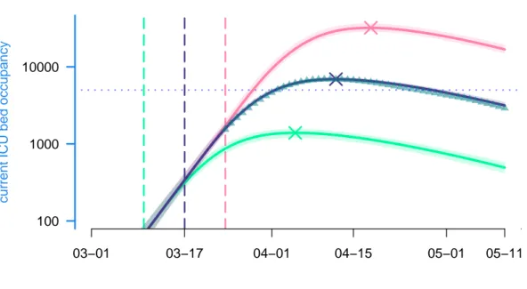
Using our estimated parameters, we then explored the effects of implementing the national lock-down a week earlier or a week later. As shown in Figure 4, the peak was reached on Apr 8, with 7019 ICU beds occupied (the model estimates it to Apr 12 and 6920 beds). Enforcing the lock-down a week earlier (in green) would have led to an earlier and smaller epidemic peak with less than 1,500 ICU beds occupied on Apr 5. Conversely, another week of delay (in red)
330
would have led to a peak above 32,000 beds occupied in ICU on Apr 18, which is largely above the ICU capacity at the time (approximately 5,000 beds). Overall, in the range studied, each elapsed week multiplies ICU occupancy peak by more than 4.5, while delaying it by 3 weeks.
These differences also translate in terms of mortality. Implementing the lock-down a week earlier could have led, according to the model, to 13,300 [12,900-13,700] less deaths, while
335
waiting for an additional week could have claimed 52,800 [45,800-61,500] more lives (Figure S-6).
100 1000 10000
current ICU bed occupancy
03−01 03−17 04−01 04−15 05−01 05−11
Figure 4: Lock-down implementation date effect and ICU bed occupancy
Each curve represents the median current ICU bed occupancy as generated by the model according to a given lock-down scenario, while their surrounding shaded areas correspond to the their 95% confidence interval. From bottom to top: the green scenario simulates an early national lock-down (on Mar 10th); the purple scenario is the realised one (lock-down beginning on Mar 17); the pink scenario simulates a late lock-down (on Mar 24th). Vertical lines indicate lock-down implementation dates. Crosses indicates the median ICU peak activity. Triangles represent the data and the dotted line the maximum ICU bed capacity in France.
3.3
Predicting future dynamics
This model cannot estimate the effects of the end of the national lock-down in France on May 11, as it relies on data notifying events that occur on average two (ICU admission) to four (death)
340
weeks after contamination. However, assuming our estimated value hold after the lock-down is ended, we can explore the future dynamics as a function of the post-lock-down reproduction number. The aim is not to make predictions, since there is no data to test them, but rather to highlight the interplay between the post-lock-down reproduction number and NPI-enforcement timing with respect to a potential epidemic rebound. For illustration purposes, the chronicles
345
of four scenarios are provided in Appendix S3.4.
We also provide a graphical online interface (provided as a supplementary data) to maximise the reach of the model.
the effect of the NPI reinforcement delay on the ICU peak height and timing. The results are
350
shown in Figure 5. As expected, a reproduction number less or equal to 1 (in green) does not require any control reinforcement. Conversely, higher values of Rttrigger an epidemic rebound,
that can saturate France’s ICU capacity (ca. 5,000 regular beds) with values as low as 1.2 [1.1, 1.3] if an appropriate control response is not implemented before mid-July. For Rt ≥ 1.3, we find that a reinforcement as early as mid-June is necessary to preserve the national health
355
system (Figure 5, top panel). Additionally, Figure 5 (bottom panel) shows that if a massive peak is to occur (Rt≥1.7), it will likely be in the second part of July, even if an appropriate response in mounted in mid-June or later. For lower peaks (Rt < 1.5), the height of which can be substantially reduced by timely reinforcement of control, occur within one month (early responses) to two weeks (late responses) after NPI implementation.
Figure 5: Effect of reproduction number and NPI response on ICU peak dynamics. Colors indicate post-lock-down reproduction number, which ranges from 1 (green) to 2.1 (brown) (see the legend with the 95%-CI). The abscissa indicate the date of implementation of renewed NPI that bring the reproduction number to Rt=0.91 [0.85, 0.98]. Each dot represents the median highest number of ICU occupied beds (top panel) and the median date at which the peak is reached (bottom) (the bars indicate the 95% CI). Dots at the bottom of each panel correspond to an absence of epidemic rebound (therefore the peak is artificially considered to be on May 12). The vicinity with the threshold value 1 for Rt explains the large CI of the peak
dates for the green and turquoise scenarios.
3.4
Comparing intervention strategies
In this section we use the model previously fitted on the data available as of May 12 to explore control strategies that belong to three main classes of non-pharmaceutical interventions (NPI): adaptive (indicator-triggered) lock-down, periodic alternation of lock-down and release phases (not indicator-triggered), and age-differential control.
We compare scenarios using the predicted cumulative hospital mortality on Dec 31 2020. The choice of this criterion is motivated by three reasons. First, the mortality time series is the one captured with the greatest accuracy by the model. Second, in the absence of pharmaceutical solutions, deaths are a more stable indicator of the state of the epidemic (e.g. the timing of hospitalizations may change as knowledge of the disease accumulates). Third, peak ICU activity
370
and concern is more likely to vary among countries, which makes it less generic.
Importantly, the following simulations are in no way intended to be statistical forecasts of the COVID-19-related death toll at the end of 2020 in France or elsewhere, but rather a numerical illustration of the non-trivial interplay between the degrees of freedom in each of the NPI strategies considered. For the sake of parsimony, we set the implementation of all
375
further considered strategies by May 12, thus avoiding to consider multiple scenarios between lock-down lifting and new NPI reinforcement (this aspect having been addressed above).
To facilitate the comparison in terms of control burden of the following strategy, we hereafter reason in terms of per capita contact ratio (PCCR), denoted by c. This dimensionless number aims to quantify the average potentially infectious contacts an individual has per unit of time,
380
relative to the pre-epidemic baseline (see AppendixesS2.2and S2.3for more details about how
cis formally introduced in the model). This definition has the following consequences:
• the average PCCR before lock-down is cpre-lock=1,
• under the proportionate mixing assumption, the encounter rate at date t of two individuals belonging to age groups i and j respectively is proportional to ci(t) cj(t),
385
• the average PCCR during the lock-down is clock = √
1 − κ = 50% [48, 52] %, where κ is the lock-down control coefficient,
• the threshold PCCR value corresponding to a reduction of the reproduction number to exactly 1 is ct= R
−1 2
0 =58% [56, 60] %.
By standardizing the control parameters of the model on a relative scale, the PCCR allows us
390
to perform comparisons of control strategies that are independent from the estimated (past) or arbitrary (scenarios) values of both basic and temporal reproduction numbers. In addition, it provides an easy way to picture the control burden of each strategy. Indeed, the average
’pre-lock-down’, situation). Between these two extremes, the remarkable value ct demarcates
395
the threshold above which an epidemic rebound is made possible.
Notice that this formalism caputres both reduction in contact rate (e.g. working from home) and probability of transmission per contact (e.g. wearing a mask).
3.4.1 Adaptive lock-down
The adaptive lock-down popularised by Ferguson et al. (2020) consists in triggering a
lock-400
down (or possibly other broad restrictive measures) if an epidemic rebound is detected by a relevant indicator. This requires to carefully identify the threshold above which the lock-down is triggered. FollowingFerguson et al.(2020), we use ICU admissions to quantify this threshold because they achieve a good balance between reflecting the epidemiological dynamics in the general population (the sampling of newly infected individuals is more homogeneous than with
405
testing) and limiting the delay between the data and the state of the epidemics (we estimate this delay to be 2 weeks, while we estimate 4 weeks for mortality data).
Figure 6 shows that cumulative mortality is exponentially correlated with the daily ICU admission threshold, over the investigated range. As a consequence, there is no remarkable inflexion point that would justify a particular value, which would leave decision makers to
410
coldly balance socio-economical costs (implied by low thresholds) with potentially saved lives (endangered by higher thresholds). Such a question is once again out of the scope of the present work.
● ● ● ● ● ● ● ● ● ● ● ● ● ● ● ● ● ● ● ● ● 20000 30000 40000 50000 60000 70000 80000 cum ulativ e mor tality 5 15 40 80
daily ICU admission threshold
Figure 6: Adaptive lock-down threshold impact
Each dot represents a simulation of the model with adaptive lock-down implemented from May 12. The abscissa show the lock-down triggering threshold in terms of daily ICU admissions nationwide. The ordinate represents the median final death toll by the end of the year, along with their 95%-confidence intervals. Lock-down lifting threshold variation has negligible impact on the results (not shown here).
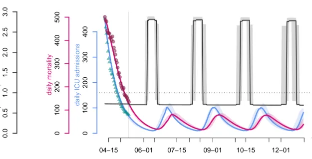
Figure 7 illustrates the chronicles produced by an adaptive lock-down strategy triggered by a threshold as low as 15 nationwide ICU admissions the same day. The epidemic can be
415
efficiently controlled on the long run this way, at the cost of approximately 50 days of lock-down to only 12 days of release per cycle, that is ca. 20% of full release time, which is less than the proportion mentioned by Ferguson et al. (2020). This relaxation proportion could however be increased if moderate measures are still implemented between lock-down phases.
0
100
200
300
400
daily ICU admissions
0 100 200 300 400 500 daily mor tality 0.0 0.5 1.0 1.5 2.0 2.5 3.0 tempor al reproduction n umber 04−15 06−01 07−15 09−01 10−15 12−01
Figure 7: Adaptive lock-down waves.
For the sake of clarity, only three parameter sets, chosen at random among the pool, illustrate here the dynamics generated by an adaptive lock-down strategy. In this scenario, the on and off thresholds are set to 15 daily ICU admissions nationwide. Symbols as in Fig.2.
3.4.2 Periodic lock-down
420
By definition, an epidemic remains under control if Rt is kept below 1. If control measures
alternate according to some periodic pattern, the instantaneous value of Rt is of little interest
and we consider instead its average value over one cycle of interventions, denoted by Rt. For
the sake of simplicity, we consider a NPI that alternates between a hard phase (typically, a lock-down) and a relaxed (or release) phase, independently from any field indicator. Let us
425
denote by cr and ch the average per capita contact ratio during the relaxed and hard phase respectively and pr the time proportion of each NPI cycle allowed to the relaxed phase.
The epidemic is under control if
Rt= (prc2r + (1 − pr)c2h) R0 ≤1. (2) The NPI cycle can contain more than two phases, but one can always pool them into those favorable to social and economic life, represented by the couple (cr, pr), and those concentrating the necessary public health restrictions, namely the couple (ch,1 − pr).
Assuming that hard phases have the same effect as the first lock-down, we can set c2
h=1 − κ (see Appendix S2.3). Then, the maximum proportion of time allowed to the relaxed phase is given by pr,max= R−10 +κ −1 c2 r +κ −1 , (3)
which is a decreasing function of cr. This expression captures the intuitive trade-off, shown in Figure S-8, which is that the lower the control in the relaxed phases, the shorter they can be. If there is no control in the relaxed phase (cr =1), then, based on our estimates for R0 and κ (Table S-5), controlling the epidemics requires that hard control be implemented 88% of the time.
435
Here, we maximize the product between intensity and duration (pr,maxcr) because it partly captures the absolute degree of freedom for a fixed period of time (i.e. try to be the less constrained as possible for the longest time period as possible). Noticing that d
dcr(pr,maxcr) <0
leads to the conclusion that the optimum is to seek for the lowest per capita contact ratio, which is obtained by setting equation 3 equal to 1. This yields c⋆
r = ct = R −1
2
0 (which equals
440
approximately 58% for R0=3). Under these conditions, there is no need for any harder phase. Importantly, the simple product pr,maxcr does not need to be the objective quantity to maximize and parametrizations of pα
r,maxc
β
r, with α, β > 0, based on socio-economical arguments, should be investigated. However, this question is out of the scope of the present work.
20000 25000 30000 35000 40000 7 14 30 60
NPI cycle duration (days)
cum
ulativ
e mor
tality relaxed per capita contact ratio
0.59 0.65 0.7 0.8
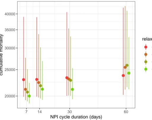
Figure 8: Effect of NPI cycle duration on cumulative mortality.
We show the cumulative mortality by the end of the year 2020 if a periodic control is imple-mented from May 12. For each of the four NPI cycle durations, the model is run for four values for cr shown in different colors, with a proportion of time satisfying eq. 3(truncated to an integer number of days). For example, in the red scenario, pr,max(0.59) = 88%, so for the weekly cycle the relaxed phase was set to floor (0.88 ⋅ 7) = 6 days.
Up to now we only investigated the proportion of the time spent in a relaxed or hard control
445
phase. However, a 0.5 proportion can correspond to a 1 week / 2 week periodicity or to a 1 month / 2 month periodicity. In fact, the trade-off relation shown in Figure S-8 theoretically works for any time split where a proportion pr,max is spent in a relaxed phase with per capita contact ratio cr and a proportion 1 − pr,max) corresponds to a strong control phase where per capita contact ratio is restricted to κ. To be implemented, such periodic control should consider
450
phases lasting at least several days. Furthermore, a periodicity greater than a month exposes populations to a greater risk during the relaxed phase.
Figure 8 suggests that the duration of the overall cycle has an effect up to 5,000 deaths, over the explored range. A weekly cycle yields the lowest death tolls, both in terms of median and CI. Furthermore, if the period lasts a month or less, a lower control of the epidemic in
455
the relaxed phase yields the lowest cumulative mortality. Morecisely, these results shows that allowing 1 moderately relaxed (the average PCCR being equal to 80%) day per week within a prolonged lock-down has a better mortality outcome than the adaptive lock-down set with 15
daily ICU admission as a threshold (approx. 8,000 deaths less by the end of the year).
3.4.3 Age-differential control
460
Age-group targeted control measures are motivated by the age dependent risk profile (Verity et al., 2020a; Collaborative et al., 2020). However, this model could easily include other risk factors such as heart disease, diabetes, or obesity. One of the simplest strategies is to incite people at risk to stay at home. On the other side of the age pyramid, a finer age-specific strategy could be to close schools and universities. More generally, political and economical
465
incentives to telework could also be considered as age-specific control measures.
We divided the population into three groups according to the cut-off ages of 25 and 65 years old. The first group is motivated by the control leverage represented by school and university closure, while the third is motivated by preventing viral circulation within the age group having the highest IFR. Each age group was assigned a fixed PCCR until the end of the year: 50, 58,
470
62, 65 and 75%. This led to 125 scenarios that are shown in Figure 9. The ratio of daily interaction between two individuals relative to the pre-epidemic baseline is the product of their individual contact ratios.
The results of the numerical investigation of 3-age group-differential controls are shown in Figure9. This scatter plot shows that cumulative mortality is well explained by
demographic-475
averaged PCCR. Therefore, the variance in contact ratio among age groups (not shown on the plot) has little impact on the long-term epidemic dynamics. This result suggests that there is no easy way of taking advantage of the strong correlation between COVID-19 complication risk and age, unless implementing an unrealistically restrictive quarantine for at-risk groups.
20000 50000 1e+05 2e+05 cum ulativ e mor tality 0.5 0.6 0.7
average per capita contact ratio
Figure 9: Effect of age-differential control interventions on cumulative mortality by
the end of 2020
Each dot represents a simulation of the model with age-differential restrictions implemented after May 11. The abscissa corresponds to the demographic-weighted average in PCCR and the ordinates represent the median final death toll by the end of the year if no other solution is implemented (bars indicante 95%-CI). The color of the dots shows the temporal reproduction number by May 18: in green the epidemic is under control and the 97.5% quantile is less that 1, in purple the median is below 1 but the 97.5% quantile is above 1, in pink the median is above 1 but the 2.5% quantile is below 1, and in grey the epidemic is out of control, the 2.5% quantile is greater than 1. Vertical bars show the 95%-likelihood interval of the expected per capita contact ratio threshold above which the reproduction number is above 1, in a homogeneously-controlled population.
4
Discussion
480
COVID-19 is not an unusually lethal or contagious infectious disease. On the other hand, the large proportion of transmission attributable to individuals with few or no symptoms makes it redoubtably difficult to control compared to SARS (Fraser et al., 2004). In the absence of a massive and homogeneous screening effort, the reflection of the epidemic dynamics of COVID-19 is reduced to hospitalizations induced by complications, which are rare and occur on average
485
two weeks after infection. The marginal, indirect and delayed nature of these events justifies the use of statistical analyses and mathematical modelling in the short-term epidemiological management of this unprecedented health crisis, that challenges all components of our societies. However, given the magnitude of the risks at stake, the diversity of fields involved, and the number of unknowns (such as climate effects, immunity duration), mathematical modelling
490
predictions should be handled with caution in the decision process.
Informing decision making represents a challenge because most mathematical modelling in epidemiology relies on continuous time deterministic models. These offer a wide palette of analytical tools, but they also become less accurate on short time scales. Conversely, stochastic models, whether agent based or not, offer a much more precise picture of the early stages of the
495
epidemics. However, they become less necessary once the outbreak threshold has been crossed and epidemic dynamics are essentially deterministic.
We therefore developed an original framework at the crossroads of individual-centered and compartmental modelling approaches, tailored to the COVID-19 natural history, which has two great advantages. First, its discrete time structure, shared with that of common epidemiological
500
data, allows us to assume any distribution for model processes, therefore introducing what is known in the literature as memory effects (or ‘non-Markovian’ processes), related to the age of the infection. As a result, we obtain a much better fit than classical memory-less (or ‘Markovian’) models on intermediate timescales (weeks or months). Second, the deterministic nature of the model allows us to perform extremely fast simulations, especially compared to
505
agent-based modelling that requires the drawing of millions of random numbers for a single simulation. The computational performance combined to the great parsimony, that still allows it to accurately fit the observed epidemiological dynamics, makes this model a relevant tool that can be easily transposed and deployed to other settings, countries or scales – even with
data limited to those publicly available, as it is the case in the present work.
510
First, we used our model to infer three key parameters of the epidemics. Our R0 is compa-rable to that already computed in France based on their 95% confidence interval (Di Domenico et al., 2020; Roques et al., 2020; Salje et al., 2020; Hoertel et al., 2020). We also estimate the temporal reproduction number Rt after the lock-down to 0.71, which is higher than that
estimated by earlier studies (Salje et al., 2020; Hoertel et al., 2020), and the number of lives
515
potentially saved (more than 50,000) compared to a lock-down implemented a week later. Once the parameters estimated, we investigated potential scenarios for control, based on the assumption that the major characteristics of the epidemics will not change, meaning for instance that a seasonal effect would have a limited impact on transmission dynamics. Our results suggest that, in the case of a rise of the reproduction number above the unit threshold
520
value, a reinforcement needs to be implemented within 5 weeks after lock-down lifting to prevent a massive second epidemic peak.
Then, we explore two types of cycling strategies. The first strategy, known as adaptive lock-down and popularised as ‘stop-and-go’, consists in alternating strict lock-lock-down and absence of control (Ferguson et al., 2020), the shift between the two being based on the incidence of daily
525
patient admission in ICU. We show that this requires a low threshold without a particular value standing out. The second strategy explored is the fixed-period alternation between lock-down and relaxed phases. Our work highlights that, for the adaptive lock-lock-down to perform better than the latter, both in terms of casualties and time spent under relaxed control, part of the restrictions have to be maintained between lock-downs. Besides, we investigated
age-530
differential control strategies and show that there is little public health benefit to be gained from the variance of control restrictions between age groups, unless implementing measures even more restrictive than the past lock-down. However, synergy between age differential and periodic control strategies is left to be explored.
The model makes several strong assumptions. First, there is no spatial structure. This
535
limitation can become strong if the epidemic grows in size to infect a large proportion of the population. Second, there is no specification of the public health control measures implemented: all the options (quarantine of confirmed cases, adoption of barrier measures, social distancing: closing of schools and universities, banning of gatherings, etc.) are combined to reduce the
contact rate. We also neglected fomite transmission (see Ferretti et al.(2020) for an example)
540
and assumed perfect and lifelong immunity against reinfection due to currently insufficient data on immunity. One simplifying assumption we made is that mortality probabilities do not vary over time, whereas in practice hospital saturation could affect mortality, whether related to COVID-19 or not.
In terms of outlook, this work lays the foundation for an online application soon to be
545
released, as an update of the earlier version COVIDSIM-FR (ETE Modelling Team, 2020a). Next challenges include taking to account for possible changes in parameter values with time, mainly detecting and estimating seasonal effects. If these are of significant impact, model fitting could be adapted, either by estimating parameters within defined time windows or by left-censoring the data as time goes by. Lastly, the NPI analysis exposed in this work sets
550
the ground for the exploration of finely tuned public health measures accounting for spatial heterogeneity and combining advantages of adaptive, periodic and group-differential modalities, with the aim of avoiding an epidemic rebound while minimizing its population burden.
Acknowledgements
This work is based on a report and online shiny application published online on Apr 6, 2020
555
http://bioinfo-shiny.ird.fr:3838/COVIDSIM-FR(ETE Modelling Team, 2020a).
We acknowledge support from the University of Montpellier, the CNRS and the IRD.
Competing Interests
We have no competing interests.
Authors’ Contributions
560
Model design and analysis performation: MTS Manuscript redaction: MTS, SA, YM
Data curation: BR, BE
Computational support and sofware development: BR Mathematical support: RDD, CS
565
References
Backer, J. A., D. Klinkenberg and J. Wallinga. 2020. Incubation period of 2019 novel coro-navirus (2019-nCoV) infections among travellers from Wuhan, China, 20-28 January 2020. Eurosurveillance 25(5):2000062.
570
Bolker, B. M. 2008. Ecological models and data in R. Princeton University Press, Princeton, NJ.
Bolker, B., R Development Core Team and I. Giné-Vázquez. (2020). bbmle: Tools for general maximum likelihood estimation, Technical report, R package version 1.0.23.1.
Bouadma, L., F.-X. Lescure, J.-C. Lucet, Y. Yazdanpanah and J.-F. Timsit. 2020. Severe
575
SARS-CoV-2 infections: practical considerations and management strategy for intensivists. Intensive Care Medicine 46(4):579–582.
Chen, N., M. Zhou, X. Dong, J. Qu, F. Gong, Y. Han, Y. Qiu, J. Wang, Y. Liu, Y. Wei, J. Xia, T. Yu, X. Zhang and L. Zhang. 2020. Epidemiological and clinical characteristics of 99 cases of 2019 novel coronavirus pneumonia in Wuhan, China: a descriptive study. The Lancet
580
395(10223):507–513.
Collaborative, T. O., E. Williamson, A. J. Walker, K. J. Bhaskaran, S. Bacon, C. Bates, C. E. Morton, H. J. Curtis, A. Mehrkar, D. Evans, P. Inglesby, J. Cockburn, H. I. Mcdonald, B. MacKenna, L. Tomlinson, I. J. Douglas, C. T. Rentsch, R. Mathur, A. Wong, R. Grieve, D. Harrison, H. Forbes, A. Schultze, R. T. Croker, J. Parry, F. Hester, S. Harper, R. Perera,
585
S. Evans, L. Smeeth and B. Goldacre. 2020. OpenSAFELY: factors associated with COVID-19-related hospital death in the linked electronic health records of 17 million adult NHS patients. medRxiv p. 2020.05.06.20092999. Publisher: Cold Spring Harbor Laboratory Press. Coronaviridae Study Group of the ICTV 2020. The species Severe acute respiratory syndrome-related coronavirus : classifying 2019-nCoV and naming it SARS-CoV-2. Nat Microbiol
590
pp. 1–9.
Danesh, G., B. Elie and S. Alizon. (2020). Early phylodynamics analysis of the COVID-19 epidemics in France using 194 genomes, Technical report, virological.org.
Di Domenico, L., G. Pullano, C. E. Sabbatini, P.-Y. Boëlle and V. Colizza. (2020). Expected impact of lockdown in Île-de-France and possible exit strategies, preprint, Infectious Diseases
595
(except HIV/AIDS).
Djidjou-Demasse, R., Y. Michalakis, M. Choisy, M. T. Sofonea and S. Alizon. (2020). Optimal COVID-19 epidemic control until vaccine deployment, preprint, Infectious Diseases (except HIV/AIDS).
ETE Modelling Team (2020a). COVIDSIM-FR, Technical report, covid-ete.ouvaton.org.
600
ETE Modelling Team (2020b). Estimating the basic reproduction number of the COVID-19 epidemic in France, Technical report, covid-ete.ouvaton.org.
Ferguson, N. M., D. Laydon, G. Nedjati-Gilani, N. Imai, K. Ainslie, M. Baguelin, S. Bha-tia, A. Boonyasiri, Z. Cucunubá, G. Cuomo-Dannenburg, A. Dighe, H. Fu, K. Gaythorpe, H. Thompson, R. Verity, E. Volz, H. Wang, Y. Wang, P. G. Walker, P. Winskill, C.
Whit-605
taker, C. A. Donnelly, S. Riley and A. C. Ghani. (2020). Impact of non-pharmaceutical interventions (NPIs) to reduce COVID- 19 mortality and healthcare demand, Technical
re-port, imperial.ac.uk/mrc-global-infectious-disease-analysis/covid-19/covid-19-reports/.
Ferretti, L., C. Wymant, M. Kendall, L. Zhao, A. Nurtay, D. G. Bonsall and C. Fraser. 2020. Quantifying dynamics of SARS-CoV-2 transmission suggests that epidemic
con-610
trol and avoidance is feasible through instantaneous digital contact tracing. medRxiv p. 2020.03.08.20032946. Publisher: Cold Spring Harbor Laboratory Press.
Fraser, C., S. Riley, R. M. Anderson and N. M. Ferguson. 2004. Factors that make an infectious disease outbreak controllable. Proceedings of the National Academy of Sciences 101(16):6146– 6151.
615
Hellewell, J., S. Abbott, A. Gimma, N. I. Bosse, C. I. Jarvis, T. W. Russell, J. D. Munday, A. J. Kucharski, W. J. Edmunds, S. Funk, R. M. Eggo, F. Sun, S. Flasche, B. J. Quilty, N. Davies, Y. Liu, S. Clifford, P. Klepac, M. Jit, C. Diamond, H. Gibbs and K. van Zandvoort. 2020. Feasibility of controlling COVID-19 outbreaks by isolation of cases and contacts. The Lancet Global Health p. S2214109X20300747.
Hoertel, N., M. Blachier, C. Blanco, M. Olfson, M. Massetti, M. S. Rico, F. Limosin and H. Leleu. 2020. Lockdown exit strategies and risk of a second epidemic peak: a stochastic agent-based model of SARS-CoV-2 epidemic in France. medRxiv p. 2020.04.30.20086264. Publisher: Cold Spring Harbor Laboratory Press.
Huang, C., Y. Wang, X. Li, L. Ren, J. Zhao, Y. Hu, L. Zhang, G. Fan, J. Xu, X. Gu, Z. Cheng,
625
T. Yu, J. Xia, Y. Wei, W. Wu, X. Xie, W. Yin, H. Li, M. Liu, Y. Xiao, H. Gao, L. Guo, J. Xie, G. Wang, R. Jiang, Z. Gao, Q. Jin, J. Wang and B. Cao. 2020. Clinical features of patients infected with 2019 novel coronavirus in Wuhan, China. The Lancet 395(10223):497–506. Imai, N., I. Dorigatti, A. Cori, S. Riley and N. Ferguson. (2020). Estimating the
poten-tial total number of novel Coronavirus cases in Wuhan City, China, Technical report,
630
imperial.ac.uk/mrc-global-infectious-disease-analysis/covid-19/covid-19-reports/.
Institut National de la Statistique et des Études Économiques (2020). Pyramide des âges 2020 - France et France métropolitaine, Technical report, insee.fr.
Keeling, M. J. 1999. The effects of local spatial structure on epidemiological invasions. Pro-ceedings of the Royal Society of London. Series B: Biological Sciences 266(1421):859–867.
635
Publisher: Royal Society.
Keeling, M. J. and P. Rohani. 2008. Modeling infectious diseases in humans and animals. Princeton University Press.
Kermack, W. O. and A. G. McKendrick. 1927. A contribution to the mathematical theory of epidemics. Proc. R. Soc. Lond. A 115:700–721.
640
Li, Q., X. Guan, P. Wu, X. Wang, L. Zhou, Y. Tong, R. Ren, K. S. Leung, E. H. Lau, J. Y. Wong, X. Xing, N. Xiang, Y. Wu, C. Li, Q. Chen, D. Li, T. Liu, J. Zhao, M. Liu, W. Tu, C. Chen, L. Jin, R. Yang, Q. Wang, S. Zhou, R. Wang, H. Liu, Y. Luo, Y. Liu, G. Shao, H. Li, Z. Tao, Y. Yang, Z. Deng, B. Liu, Z. Ma, Y. Zhang, G. Shi, T. T. Lam, J. T. Wu, G. F. Gao, B. J. Cowling, B. Yang, G. M. Leung and Z. Feng. 2020a. Early Transmission
645
Dynamics in Wuhan, China, of Novel Coronavirus - Infected Pneumonia. New England Journal of Medicine 382(13):1199–1207. Publisher: Massachusetts Medical Society _eprint: https://doi.org/10.1056/NEJMoa2001316.
Li, R., S. Pei, B. Chen, Y. Song, T. Zhang, W. Yang and J. Shaman. 2020b. Substantial undocumented infection facilitates the rapid dissemination of novel coronavirus
(SARS-CoV-650
2). Science 368(6490):489–493. Publisher: American Association for the Advancement of Science Section: Research Article.
Linton, N. M., T. Kobayashi, Y. Yang, K. Hayashi, A. R. Akhmetzhanov, S.-m. Jung, B. Yuan, R. Kinoshita and H. Nishiura. 2020. Incubation Period and Other Epidemiological Charac-teristics of 2019 Novel Coronavirus Infections with Right Truncation: A Statistical Analysis
655
of Publicly Available Case Data. Journal of Clinical Medicine 9(2):538.
Magal, P. and G. Webb. 2020. Predicting the number of reported and unreported cases for the COVID-19 epidemic in South Korea, Italy, France and Germany. medRxiv p. 2020.03.21.20040154. Publisher: Cold Spring Harbor Laboratory Press.
Muller, M. and DREES. (2017). 728 000 résidents en établissements d’hébergement pour
person-660
nes âgées en 2015 (Études et Résultats, n.1015, DREES), Technical report, drees.solidarites-sante.gouv.fr.
Nishiura, H., N. M. Linton and A. R. Akhmetzhanov. 2020a. Serial interval of novel coronavirus (COVID-19) infections. International Journal of Infectious Diseases 93:284–286.
Nishiura, H., N. M. Linton and A. R. Akhmetzhanov. 2020b. Serial interval of novel coronavirus
665
(COVID-19) infections. International Journal of Infectious Diseases.
R Core Team 2020. R: A Language and Environment for Statistical Computing. R Foundation for Statistical Computing, Vienna, Austria.
Roques, L., E. K. Klein, J. Papaix, A. Sar and S. Soubeyrand. 2020. Effect of a one-month lock-down on the epidemic dynamics of COVID-19 in France. medRxiv p. 2020.04.21.20074054.
670
Publisher: Cold Spring Harbor Laboratory Press.
Roux, J., C. Massonnaud and P. Crépey. 2020. COVID-19: One-month impact of the French lockdown on the epidemic burden. medRxiv p. 2020.04.22.20075705. Publisher: Cold Spring Harbor Laboratory Press.
Salje, H., C. T. Kiem, N. Lefrancq, N. Courtejoie, P. Bosetti, J. Paireau, A. Andronico, N. Hozé,
675
J. Richet, C.-L. Dubost, Y. L. Strat, J. Lessler, D. Levy-Bruhl, A. Fontanet, L. Opatowski, P.-Y. Boëlle and S. Cauchemez. 2020. Estimating the burden of SARS-CoV-2 in France. Science. Publisher: American Association for the Advancement of Science Section: Report. Santé Publique France (2020a). COVID-19 : Point épidémiologique hebdomadaire du 7 mai
2020, Technical report, santepubliquefrance.fr.
680
Santé Publique France (2020b). Données hospitalières relatives à l’épidémie de COVID-19,
Technical report, data.gouv.fr.
Stoecklin, S. B., P. Rolland, Y. Silue, A. Mailles, C. Campese, A. Simondon, M. Mechain, L. Meurice, M. Nguyen, C. Bassi, E. Yamani, S. Behillil, S. Ismael, D. Nguyen, D. Malvy, F. X. Lescure, S. Georges, C. Lazarus, A. Tabaï, M. Stempfelet, V. Enouf, B. Coignard,
685
D. Levy-Bruhl and I. Team. 2020. First cases of coronavirus disease 2019 (COVID-19) in France: surveillance, investigations and control measures, January 2020. Eurosurveillance 25(6):2000094. Publisher: European Centre for Disease Prevention and Control.
Trapman, P., F. Ball, J.-S. Dhersin, V. C. Tran, J. Wallinga and T. Britton. 2016. Inferring
R 0 in emerging epidemics—the effect of common population structure is small. Journal of
690
The Royal Society Interface 13(121):20160288.
Verity, R., L. C. Okell, I. Dorigatti, P. Winskill, C. Whittaker, N. Imai, G. Cuomo-Dannenburg, H. Thompson, P. G. T. Walker, H. Fu, A. Dighe, J. T. Griffin, M. Baguelin, S. Bhatia, A. Boonyasiri, A. Cori, Z. Cucunubá, R. FitzJohn, K. Gaythorpe, W. Green, A. Hamlet, W. Hinsley, D. Laydon, G. Nedjati-Gilani, S. Riley, S. v. Elsland, E. Volz, H. Wang, Y. Wang,
695
X. Xi, C. A. Donnelly, A. C. Ghani and N. M. Ferguson. 2020a. Estimates of the severity of coronavirus disease 2019: a model-based analysis. The Lancet Infectious Diseases. Publisher: Elsevier.
Verity, R., L. C. Okell, I. Dorigatti, P. Winskill, C. Whittaker, N. Imai, G. Cuomo-Dannenburg, H. Thompson, P. G. T. Walker, H. Fu, A. Dighe, J. T. Griffin, M. Baguelin, S. Bhatia,
700
A. Boonyasiri, A. Cori, Z. Cucunubá, R. FitzJohn, K. Gaythorpe, W. Green, A. Hamlet, W. Hinsley, D. Laydon, G. Nedjati-Gilani, S. Riley, S. v. Elsland, E. Volz, H. Wang, Y. Wang,
X. Xi, C. A. Donnelly, A. C. Ghani and N. M. Ferguson. 2020b. Estimates of the severity of coronavirus disease 2019: a model-based analysis. The Lancet Infectious Diseases.
Wilks, S. S. 1938. The Large-Sample Distribution of the Likelihood Ratio for Testing Composite
705
Hypotheses. The Annals of Mathematical Statistics 9(1):60–62. Publisher: Institute of Mathematical Statistics.
Appendix
Table of Contents
5
S1 Mathematical notations 2
S2 Model details 5
S2.1 Recurrence relation system . . . 5
S2.2 Force of infection . . . 5 S2.3 Lock-down effect . . . 7 10 S2.4 Times series . . . 9 S2.5 Criticality-related probabilities . . . 9 S2.6 Waiting times . . . 13
S2.7 Fitting and estimation procedure . . . 15
S2.8 Derived outputs . . . 16
15
S2.9 Continuous time model . . . 18
S3 Supplementary Results 19
S3.1 Maximum likelihood parameter estimates . . . 19
S3.2 Data right censoring and parameter inference . . . 20
S3.3 Lock-down implementation date and cumulative mortality . . . 23
20
S3.4 Examples of post-May 11 scenarios . . . 24
S3.5 Time vs intensity trade-off of the relaxed phase in the periodic lock-down
strategy . . . 25
S1
Mathematical notations
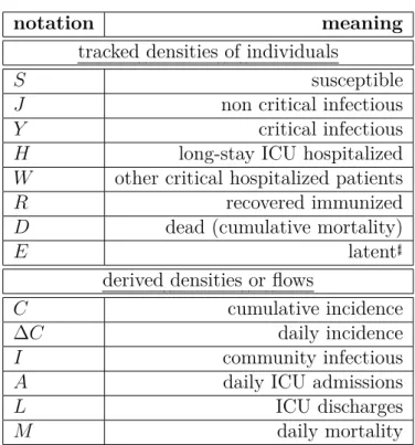
Summary table with all the notations used in the study.
notation meaning
tracked densities of individuals
S susceptible
J non critical infectious
Y critical infectious
H long-stay ICU hospitalized
W other critical hospitalized patients
R recovered immunized
D dead (cumulative mortality)
E latent♯
derived densities or flows
C cumulative incidence
∆C daily incidence
I community infectious
A daily ICU admissions
L ICU discharges
M daily mortality
Table S-1: Density related notations.