HAL Id: hal-00316969
https://hal.archives-ouvertes.fr/hal-00316969
Submitted on 1 Jan 2002
HAL is a multi-disciplinary open access
archive for the deposit and dissemination of
sci-entific research documents, whether they are
pub-lished or not. The documents may come from
teaching and research institutions in France or
abroad, or from public or private research centers.
L’archive ouverte pluridisciplinaire HAL, est
destinée au dépôt et à la diffusion de documents
scientifiques de niveau recherche, publiés ou non,
émanant des établissements d’enseignement et de
recherche français ou étrangers, des laboratoires
publics ou privés.
A case study of HF radar spectral width in the post
midnight magnetic local time sector and its relationship
to the polar cap boundary
E. E. Woodfield, J. A. Davies, P. Eglitis, M. Lester
To cite this version:
E. E. Woodfield, J. A. Davies, P. Eglitis, M. Lester. A case study of HF radar spectral width in the
post midnight magnetic local time sector and its relationship to the polar cap boundary. Annales
Geophysicae, European Geosciences Union, 2002, 20 (4), pp.501-509. �hal-00316969�
Annales
Geophysicae
A case study of HF radar spectral width in the post
midnight magnetic local time sector and its relationship
to the polar cap boundary
E. E. Woodfield1, J. A. Davies1, P. Eglitis2, and M. Lester1
1Department of Physics and Astronomy, University of Leicester, Leicester, LE17RH, UK
2Swedish Institute of Space Physics, Uppsala Division, Box 537, S-751 21 Uppsala, Sweden, and The Finnish Meteorological
Institute, P. O. Box 503, Fin-00101 Helsinki, Finland
Received: 29 May 2001 – Revised: 24 October 2001 – Accepted: 31 October 2001
Abstract. The aim of this paper is to advance the current
understanding of the spectral width parameter observed by coherent high frequency (HF) radars. In particular, we ad-dress the relationship of a frequently observed gradient, be-tween low (<200 m/s) and high (>200 m/s) spectral width, to magnetospheric boundaries. Previous work has linked this gradient in the spectral width, in the nightside sector of mag-netic local time, to the Polar Cap Boundary (PCB), and also to the boundary between the Central Plasma Sheet (CPS) and the Plasma Sheet Boundary Layer (PSBL). The present case study investigates the former by comparison with the 630.0 nm optical emission. No suitable data were available to test the second of the two hypotheses. It is found that during the interval in question the spectral width gradient is within the region of the 630.0 nm optical emission. A com-parison of coherent and incoherent scatter radar data is also conducted, which indicates that values of high spectral width are typically collocated with elevated F-region electron tem-peratures. We conclude that the high spectral width region in the interval under study is associated with particle precipita-tion and also that the spectral width gradient is not a reliable method for locating the PCB.
Key words. Ionosphere (auroral ionosphere; ionospheric
ir-regularities)
1 Introduction
The magnetosphere is dynamic and the locations of differ-ent plasma regimes within it evolve continually. The bound-aries between the different regimes can move, for example, in response to coupling between the interplanetary magnetic field (IMF) and the geomagnetic field, and magnetospheric substorms. In order to study the dynamical processes in the magnetosphere it is necessary to follow the dynamics of the plasma regimes. Many of the processes that occur in the
Correspondence to: E. E. Woodfield
(Emma.Woodfield@ion.le.ac.uk)
magnetosphere leave signatures in the ionosphere that can be observed either from the ground or from space. Detecting and tracking the ionospheric signatures of magnetospheric processes is a task ideally suited to ground-based instruments because of their large spatial and temporal coverage.
Of particular interest in the magnetosphere is the open/closed field line boundary (OCFLB). At ionospheric altitudes this is often referred to as the polar cap boundary (PCB), the polar cap being the region in the ionosphere that maps to open field lines in the magnetosphere. Several iono-spheric proxies have been suggested for locating the PCB (e.g. Blanchard et al., 1995; Doe et al., 1997; Rodger, 2000). Blanchard and co-workers used DMSP satellite data to show that a well-defined step in the intensity of the 630.0 nm emis-sion at its poleward edge locates the PCB to an accuracy of ±0.9◦invariant latitude in the pre-midnight sector. This step indicates the change from high-energy precipitation on closed field lines to the low energy, diffuse polar rain ob-served within the polar cap itself.
Recent work has suggested that a marked gradient between areas of high (>200 m/s) and variable, and low (<200 m/s) Doppler spectral width values measured by HF radars can also be used as a proxy for the PCB on the nightside, since in the case presented by Lester et al. (2001), it follows the pole-ward edge of the 630.0 nm emission in the pre-midnight sec-tor. This spectral width gradient occurs frequently in radar data both on the day and nightside (Baker et al., 1995; Du-deney et al., 1998; Andr´e et al., 1999). On the dayside, the region of high spectral width poleward of the spectral width gradient is a well-known signature of the cusp (e.g. Baker et al., 1995; Andr´e et al., 1999; Milan et al., 1999). On the nightside, in addition to the PCB, the spectral width gradi-ent has been linked to the magnetospheric boundary between the central plasma sheet (CPS) and plasma sheet boundary layer (PSBL) (Lewis et al., 1997; Dudeney et al., 1998). This boundary is located between two regions of closed field line plasma and will, therefore, map into the ionosphere equator-ward of the PCB.
re-502 E. E. Woodfield et al.: A case study of HF radar spectral width in the post midnight magnetic local time sector gions of high spectral width have been suggested.
Simula-tion runs through standard HF coherent radar analysis soft-ware have shown that high spectral width values can be gen-erated by broadband wave activity in the Pc1/Pc2 frequency band (Andr´e et al., 1999, 2000a). The presence of suitable waves has been verified by satellite measurements of the cusp that show a step-like increase of wave activity in the fre-quency band 0.2–2.2 Hz with electric field measurements of a few mV/m, coincident with cusp particles (e.g. Maynard et al., 1991; Matsuoka et al., 1993). On the nightside, elec-trostatic wave activity of a similar frequency range (assumed to be driven by electron precipitation) increases across the CPS/PSBL boundary (Dudeney et al., 1998). Work by Schif-fler et al. (1997) and followed up by Huber and Sofko (2000) has found SuperDARN double-peak spectra in the region of the low-latitude boundary layer (LLBL). These would naturally lead to high spectral widths. They attribute the generation of these double-peak spectra to small-scale vor-tices (<26 km and <4 s lifetime) which are smaller than the normal spatial and temporal resolution of the SuperDARN radars. They suggest that these vortices may be formed in one of two ways. Ion precipitation spreads radially through charge exhange collisions as it travels downwards in the ionosphere (Davidson, 1965). Thus, if it is co-located with electron precipitation (which does not suffer the same effect), a radial electric field will be produced and hence, a vortex will be the result. Alternatively, vortices may form as a result of the Kelvin-Helmholtz instability to be found at velocity shears, which, when located within a range cell, would them-selves be expected to produce a spectrum with more than one peak (Andr´e et al., 2000b). Andr´e et al. (2000b) also mod-elled the effect of a small vortex on the standard SuperDARN fitting software and concluded that a vortex smaller than 5 km would not generate a clear multi-component spectrum in the radar data.
In this case study from 20 December 1998, one of the CUTLASS (Co-operative UK Twin Located Auroral Sound-ing System) coherent HF radars, part of the SuperDARN net-work (Greenwald et al., 1995), is used to show that a gradient between low and high variable spectral width is not neces-sarily a good proxy for the open/closed field line boundary on the nightside. We also demonstrate that elevated electron temperatures caused by particle precipitation in the F-region may be related to the region of high variable spectral width during this period.
2 Experimental overview
The CUTLASS pair is the eastern most pair of the Super-DARN network (Greenwald et al., 1995). The two CUT-LASS radars are located at Pykkvibær, Iceland (64.5◦N, 68.5◦E geomagnetic-altitude adjusted corrected geomag-netic (AACGM) coordinates based on Baker and Wing (1989) will be employed hereafter) and at Hankasalmi, Fin-land (58.6◦N, 104.9◦E). Both radars scan through 16 az-imuthal beams arranged symmetrically about the radar bore
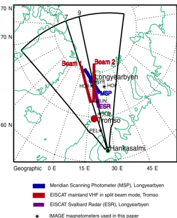
7 9 60 N 70 N 70 N 0 E 15 E 30 E 45 E Hankasalmi Tromso Longyearbyen Beam 1 Beam 2 Geographic MSP ESR
Meridian Scanning Photometer (MSP), Longyearbyen EISCAT mainland VHF in split beam mode, Tromso EISCAT Svalbard Radar (ESR), Longyearbyen IMAGE magnetometers used in this paper
LYR HOP BJN SOR PEL HOR
Fig. 1. Map indicating the location of the fields-of-view of the in-struments used in this study. Only the IMAGE magnetometer sta-tions referred to in the text are plotted.
site. In the standard operating mode the dwell time on each beam is typically 7 s and the scan starts every two minutes in standard common mode operation. Each beam is separated into 75 range gates. In standard common mode these range gates are 45 km in length with a distance to the first gate of 180 km. The radars can operate at frequencies between 8 and 20 Mhz. The fields-of-view of the two radars overlap to fa-cilitate bistatic velocity measurements.
The radar field-of-view covers some 4×10⁶km2, although often only a proportion of this area produces ionospheric backscatter. There are two reasons for this, the first being that HF radio propagation in the ionosphere does not uniformly illuminate the region. Secondly, if there are no field-aligned irregularities, then there will be no targets to scatter from and hence, no backscatter. Therefore, care is required in deduc-ing geophysical data from boundaries of backscatter, since the edge may be due to the end of the region illuminated by the radar and not the edge of the location of field-aligned ir-regularities. However, in this interval, the boundary in ques-tion is in the middle of a region of powerful backscatter from similar elevation angles and can, therefore, be assumed to be due to a change in the physical characteristics of the irregu-larities being observed.
In this study we only use Finland radar data, and the field-of-view from Hankasalmi is shown in Fig. 1. The radar was performing 7 s dwell time scans on each beam with standard common mode range gates, although the beam direction
re-verted to beam 5 after each other beam to give a higher time resolution for beam 5 until 05:00 UT when the scan resumed its normal consecutive order. The time resolution for beam 9 from 01:00 UT to 05:00 UT was 224 s and from 05:00 UT to 06:00 UT it was 120 s. During the dwell time, when sound-ing in a particular beam direction, the radar transmits a 7-pulse sequence repetitively (approximately 10 multi-7-pulse sequences can be transmitted each second). Samples of the returned signal are taken, correlated and integrated, so as to give the auto-correlation function of the scattered signal for each range gate. As described more fully by Villain et al. (1987), the signal power, the rate of change of phase an-gle and the rate of decay of the auto-correlation function are parameterized, leading to an estimate of backscatter power, line-of-sight velocity and spectral width, respectively, of the particular scattering targets occupying each radar range gate. The spectral width is the particular parameter of interest in this paper. It is strictly a measure of the correlation time of the radar signal. For example, the scattering properties of the ground remain fairly uniform with time and hence, the spectral width of ground scatter is typically small. For ionospheric scatter the coherence in the signal and hence, the spectral width is normally related to the variation in the plasma flow in the radar scatter volume. In this paper, we concentrate on identifying specific regions of radar scatter that have a characteristic spectral width.
Observations from two of the European Incoherent SCAT-ter (EISCAT) radars have also been included in this work (Rishbeth and Williams, 1985). The VHF radar at Tromsø (66.4◦N, 103.5◦E) and the UHF EISCAT Svalbard Radar (ESR) (75.0◦N, 113.0◦E), (Wannberg et al., 1997) provide estimates of a variety of plasma parameters including elec-tron temperature and ion velocity. The VHF radar at Tromsø was operating in split beam mode for the majority of the in-terval 01:00 to 06:00 UT on 20 December 1998; the two pole-ward pointing beams are shown in Fig. 1. Beam one has an azimuth of 345.0◦clockwise to geographic north and beam two has an azimuth of 359.5◦. Also shown is the equator-ward pointing ESR beam which has an azimuth of 161.6◦. All three beams were at an elevation of 30.0◦. Only data from the modes of operation described above are included in this investigation.
Optical observations from the meridian scanning pho-tometer (MSP) at Longyearbyen on Svalbard (75.0◦N, 113.0◦E, AACGM) are employed. The MSP observes at four different wavelengths, 427.8 nm, 486.1 nm, 557.7 nm and 630.0 nm. Only the 557.7 nm (green line) and 630.0 nm (red line) emissions are utilised in this study. The photometer scans from an elevation of 0◦, at an azimuth of 45◦, to 0◦ el-evation at an azimuth of 225◦. Each scan takes two seconds and repeats every 16 s.
Observations from the IMAGE network of magnetome-ters (Viljanen and Hakkinen, 1997) supply information about ionospheric currents during the interval. The locations of the IMAGE stations employed in this paper are also plotted in Fig. 1. -6 -4 -20 2 4 6 B x (n T ) -6 -4 -2 0 2 4 6 B y (n T ) -6 -4 -20 2 4 6 B z (n T ) 360 380 400 420 6 8 10 12 1.5 2.0 2.5 3.0 3.5 P re ss ur e (n P a) 0100 0200 0300 0400 0500 UT V el oc ity ( m s -1) D en si ty ( cm -3) 0600
Fig. 2. Solar wind and IMF data from the WIND SWE and MFI instruments on 20 December 1998. The times shown are at the spacecraft, a time delay of ∼ 10 min to the ionosphere has been calculated. The top three panels display components of the inter-planetary magnetic field in GSM coordinates. The bottom three panels indicate solar wind bulk velocity, density and pressure,
re-spectively. WIND was located at approximately (40 RE, 60 RE,
10 RE), (X, Y, Z) in GSM coordinates during this interval.
3 Observations
3.1 Interplanetary conditions
The interval under investigation takes place on the morning of 20 December 1998, from 01:00 UT to 06:00 UT. The IMF and solar wind data taken by the MFI (Lepping et al., 1995) and SWE (Ogilivie et al., 1995) instruments on the WIND spacecraft are shown in Fig. 2. The spacecraft was located at (40 RE, 60 RE, 10 RE), (X, Y, Z) in GSM coordinates from which point a time delay of ∼ 10 min from the satel-lite to the magnetopause has been estimated. This time delay has not been added to any of the times referred to for the spacecraft. The z component of the interplanetary magnetic field (Bz) is northwards at the spacecraft from 00:30 UT un-til 02:25 UT, when it becomes weakly southward at first and then more strongly southward after 02:50 UT. At 03:00 UT,
Bz then returns northward until 03:40 UT when it becomes variable until 05:35 UT, after which it becomes increasingly southward. The y component (By) is positive until a sudden, large jump from +6 nT to −6 nT at 02:20 UT. It is variable after this until another extended period of positive values be-gins at 04:35 UT. The x component Bx is approximately in antiphase with Bythroughout the interval.
504 E. E. Woodfield et al.: A case study of HF radar spectral width in the post midnight magnetic local time sector
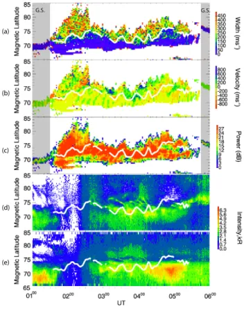
Fig. 3. HF radar data from CUTLASS Finland beam 9, 20 De-cember 1998, (a) Doppler spectral width, (b) line-of-sight velocity (blue is towards the radar), (c) backscatter power. MSP data from Longyearbyen, (d) 630.0 nm, red emission, from an assumed al-titude of 250 km, (e) 557.7 nm, green emission, from an assumed altitude of 110 km. All 5 panels have the spectral width gradient at 200 m/s overlaid on them in white for comparison. The intervals marked “G.S” have been identified as ground scatter.
∼350 km/s at 00:00 UT to ∼ 420 km/s at 03:30 UT, after which it decreases to ∼ 400 km/s. The density and pressure values indicate a trough between 01:20 UT and 02:20 UT with the density decreasing sharply from 12 cm−3to 7 cm−3. At 02:20 UT, the density and pressure recover quickly to their previous levels where they remain until 05:20 UT when an-other sharp decrease is observed.
3.2 CUTLASS data
The Doppler spectral width, line-of-sight irregularity drift velocity and backscatter power from beam 9 of the Finland radar from 01:00 UT to 06:00 UT on 20 December 1998, are shown in panels (a) to (c) of Fig. 3 (positive velocities are directed towards the radar). To convert UT to magnetic lo-cal time (MLT) in the region of magnetic latitude covered by the CUTLASS Finland field-of-view, add approximately 2.5 h to the UT. F-region backscatter is observed from 02:00 to 05:00 UT northward of 65◦N during this time. The scat-ter shown between 01:00 UT and 01:30 UT, and also from 05:45 UT to 06:00 UT, has been identified as ground scatter
20 30 40 50 60 R an g e G at e 0 100 200 300 400 500 Spectral Width (ms-1) % O cc u rr en ce 0 1 2 3 4 5 6 7 8 9 (67.5oN) (83.0oN)
Fig. 4. A contour plot of spectral width distributions for beam 9,
range gates 20 (∼ 67.5◦N) through 60 (∼ 83.0◦N) for the interval
01:30 UT to 05:30 UT. The colour scale indicates percentage occur-rence with the distributions normalised to the total number of obser-vations from each range gate. The very low spectral width values are not due to ground scatter.
using elevation angle data. The SuperDARN radars typically identify data with spectral widths below 20 m/s and veloc-ity magnitude below 50 m/s as arising due to ground scat-ter. In general, this approach is highly effective. However, for the particular F-region scatter interval between 01:30 UT and 05:30 UT of interest here, the standard method led to the misidentification of some of the ionospheric scatter between 68◦N and 75◦N as ground scatter. Consequently all ground scatter was identified by studying the elevation angle data. The F-region backscatter power, panel (c) of Fig. 3, is con-sistently high throughout the interval 02:00 UT to 05:00 UT. The position of the poleward edge of the F-region backscat-ter varies between 73◦and 84◦, while the equatorward edge remains fairly static between 67◦and 69◦.
In the Doppler spectral width data, Fig. 3a, there is an area of low spectral width (< 200 m/s) equatorward of a large area of high (> 200 m/s) but variable spectral width. A typically sharp nightside gradient in width, ∼ 60 ± 30 m/s/degree, ex-ists between these two regions and is shown by the white line in Fig. 3a. This boundary has been overlaid on all the other panels of Fig. 3 for comparison. A plot of the spectral width distributions for each range gate from 20 to 60, covering a latitude range from 67.5◦N to 83.0◦N, is shown in Fig. 4. A bin width of 20 m/s has been used. The data are taken from the interval of F-region scatter from 01:30 UT to 05:30 UT and have been normalized to the total number of observa-tions in each range gate. The very low spectral widths are not a result of ground scatter since the time interval and range gates chosen contain only F-region scatter. There is an ob-vious change from distributions peaked between 0 to 20 m/s
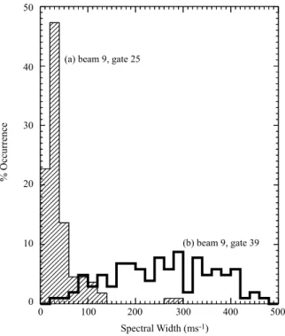
% O cc ur re nc e 0 10 20 30 40 50 0 100 200 300 400 500 Spectral Width (ms-1) (a) beam 9, gate 25
(b) beam 9, gate 39
Fig. 5. Two histograms displaying spectral width distributions for
(a) beam 9, range gate 25 (∼ 69.6◦N), and (b) beam 9, range gate
39 (∼ 75.3◦N). Each histogram is normalized to the total number
of observations from that gate.
up to range gate 30 (∼ 71◦N), to those distributions where the peak is around 250 m/s above range gate 40 (∼ 75◦N). In between 71◦N and 76◦N, a transition between these two extremes is observed; this corresponds to the latitude region within which the 200 m/s gradient moves during this inter-val. Figure 5 presents the distributions of the spectral width for range gates 25 (∼ 69.9◦N) and 39 (∼ 75.3◦N) of Fin-land beam 9 for the interval 01:30 UT to 05:30 UT; the black lines on Fig. 4 show their location. It is clear that the more northerly range gate 39 shows a much more rounded distribu-tion, with a significant percentage (∼ 66%) of spectral width values larger than 200 m/s, while range gate 25 has virtually no data points above 100 m/s. Therefore, we feel justified in using a value of 200 m/s when locating the spectral width gradient in the time series plots of Fig. 3. The form of the rounded distribution for gate 39 resembles closely that of the spectral width distribution identified by Baker et al. (1995), as being a proxy for the location of the cusp on the dayside.
The line-of-sight velocity data (Fig. 3b) indicates that the highest velocities are at the poleward edge of the F-region backscatter, and that these velocities have a component that is directed towards the radar (in blue). The strong bursts of flow with components towards the radar that occur at 03:10 UT and 03:50 UT are associated with pronounced velocity en-hancements in anti-sunward flow. There is evidence of long period wave activity (ULF) in the line-of-sight velocity data, from 02:10 UT to 04:00 UT between 69◦and 74◦. The pe-riod of the wave is approximately 10 min. We return to this
observation in Sect. 3.4.
3.3 Meridian scanning photometer data
The optical data for two wavelengths, 630.0 nm and 557.7 nm, taken from the Longyearbyen MSP for the inter-val 01:00 UT to 06:00 UT on 20 December 1998 are shown in Fig. 3d and 3e, respectively. These have been plotted as a function of magnetic latitude, assuming an altitude of 250 km for the emission at 630.0 nm and 110 km for 557.7 nm. The assumed altitudes are seen to be reasonable in the discussion. There is structure in both the 630.0 nm and 557.7 nm emis-sions from 01:00 UT until 01:40 UT when a sudden decrease to very low intensity emission occurs. This lack of emission lasts until 02:40 UT. Coincidentally, the time-span of this marked drop in intensity is the same as the density decrease observed by WIND when a time lag of 20 min from the spacecraft is included. It may be possible that the two events are related in some way, with the additional delay of 10 min a result of the reaction time in the nightside ionosphere to the change at the magnetopause. The optical intensity de-crease between 01:40 UT and 02:40 UT hails the beginning of the region of ionospheric scatter observed by the Finland HF radar. The region of ionospheric scatter expands quickly to cover latitudes from 67◦N up to 83◦N, then the pole-ward edge of it contracts dramatically just before 02:40 UT to 76◦N. The 630.0 nm emission then takes the form of a nar-row band of high intensity, i.e. above 3 kR, which is approxi-mately 2◦wide in latitude at 02:40 UT. The peak intensity of the main emission moves equatorwards from 75◦N to 71◦N, during the interval 02:40 UT to 04:20 UT. After this, the peak emission moves polewards to 77◦N, once again becoming narrow, reaching its maximum latitude at 05:40 UT. Above the main latitude of emission there are several equatorward moving features starting at 03:10 UT, 03:45 UT, 03:55 UT and 04:00 UT. The first and last of these moves from 76◦N to 73◦N, while the intermediate features move from 75◦N to 73◦N. The approximate rate of motion is 0.1◦±0.05◦per minute (∼ 170 m/s).
The 557.7 nm emission, although active simultaneously with the 630.0 nm emission, has a constant poleward edge at 73◦with a broader region of high intensity, above 3 kR, and variable structure equatorward of this latitude. The same re-duction in luminosity between 01:40 UT and 02:40 UT is ob-served in the 557.7 nm emission, as are the same equatorward moving features from 03:10 UT to 04:00 UT. The peak of the of the 557.7 nm emission is located at approximately 72◦N from 02:40 UT until 04:10 UT, when it moves southwards to 70◦N at 05:00 UT, as the intensity starts to decrease until it is beyond the interval of interest. The equatorward edge of the emission is south of the field-of-view from 02:50 UT until the end of the interval.
3.4 Magnetometer data
A 150 nT negative bay is observed in the X-component (north-south) data from Sørøya (SOR, 67.1◦N, 106.7◦E)
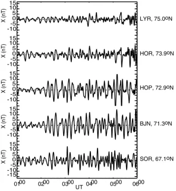
506 E. E. Woodfield et al.: A case study of HF radar spectral width in the post midnight magnetic local time sector -10-5 0 5 10 15 X (n T) -10-5 0 5 10 15 X (n T) -10-5 0 5 10 15 X (n T) -10-5 0 5 10 15 X (n T) -15 -10-5 0 5 10 15 X (n T) 0100 0200 0300UT 0400 0500 0600 LYR, 75.0oN HOR, 73.9oN HOP, 72.9oN BJN, 71.3oN SOR, 67.1oN
Fig. 6. The north-south component measurements from five of the IMAGE magnetometer stations filtered between 100 s and 1000 s, 20 December 1998.
to Pello (PEL, 63.3◦N, 105.4◦E) in the image chain from 00:00 UT to 01:10 UT (not shown). This enhanced westward electrojet decays to previous levels by 01:10 UT and is, there-fore, assumed to have no effect on the spectral width bound-ary indicated in Fig. 3a. Data from five of the magnetometers of the image chain for the period 01:00 UT to 06:00 UT on 20 December 1998 are shown in Fig. 6. The magnetome-ter data have been band pass filmagnetome-tered using a range of 100 s to 1000 s. A wave, matching the frequency of the one ob-served by the Hankasalmi radar (∼ 2 MHz), is recorded by magnetometers of the image chain starting at 02:20 UT. The amplitude of the wave observed by the magnetometers is largest at the stations of Bear Island (BJN, 71.3◦N, 108.9◦E) and Hopen Island (HOP, 72.9◦N, 115.9◦E). There is a sharp decrease in the amplitude of the wave between HOP and Longyearbyen (LYR, 75.0◦N, 113.0◦E) and a slower de-crease to the south of HOP. Measurements of the latitudinal variation of the amplitude and phase of the wave area are consistent with the wave being a field line resonance (FLR) with the resonating field line poleward of HOP and equator-ward of LYR. Since FLRs only occur on closed field lines, a lower limit for the OCFLB can be set at 72.9◦N.
3.5 Incoherent scatter data
The first three panels of Fig. 7 show the electron density, electron temperature and ion velocity, respectively, observed by the ESR from 01:00 UT to 06:00 UT. The last two pan-els of Fig. 7 present the line-of-sight velocity and spectral
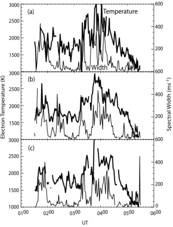
Fig. 7. Data from the EISCAT Svalbard Radar, 20 December 1998, (a) electron density, (b) electron temperature, (c) ion velocity. Data from CUTLASS Finland on a reduced latitude scale from Fig. 3, (d) line-of-sight velocity and (e) spectral width “G.S” denotes intervals of ground scatter.
width from beam 9 of CUTLASS Finland for the same range of magnetic latitudes. The ESR UHF beam was pointing in the same vertical plane as beam 9 of CUTLASS Finland, in the opposite sense during this interval, at an elevation of 30◦. The altitude range covered by the data in Fig. 7 is from ap-proximately 90 km at 74◦N to 390 km at 70◦N. Although not shown here, the data from the EISCAT VHF beams show very similar results to those from the ESR. It is evident from Fig. 7c and 7d that the line-of-sight ion velocities from the incoherent radar agree well with the irregularity drift veloci-ties observed by CUTLASS Finland. (Note that all the data shown have positive velocities towards the HF radar at Fin-land and that the range of magnetic latitudes shown is dif-ferent from Fig. 3). This is consistent with previous results that the phase speed of F-region irregularities is equal to the component of the ambient plasma flow in their direction of propagation (Davies et al., 2000 and references therein). One can observe the same field line resonance signature as seen from Hankaslami and the same flow bursts at 03:10 UT and 03:50 UT.
Equatorward moving structures are evident in the electron density and electron temperature data, Fig. 7a and 7b, re-spectively, from 03:40 UT to 04:10 UT. These structures are observed by the ESR, while equatorward moving structures are also observed by the MSP, although not simultaneously and at a lower latitude. The equatorward motion is observed at the same time as strong velocity towards Hankaslami, and
1400 1800 2200 2600 3000 (a) 0 2 4 6 8 10 12 14 N o. of oc cu rre nc es 1400 1800 2200 2600 3000 E le ct ro n T em pe ra tu re ( K ) (b) 0 100 200 300 400 500 Spectral Width (ms-1) 1000 1400 1800 2200 2600 3000 (c)
Fig. 8. Scatter plots of electron temperature from the incoherent scatter radar data against spectral width from CUTLASS Finland.
The data used has been restricted to between 71◦N and 72◦N. The
colours indicate the frequency of observations within the bin they outline.
also in the latter part of the interval when the spectral width gradient moves equatorward.
The ESR observed two pronounced regions of structured, elevated electron temperature in the F-region, Fig. 7b, and this is replicated by the two VHF beams from Tromsø, from 01:00 UT and 01:45 UT, and 03:10 UT and 04:20 UT, Fig. 7b. The ESR beam is at F-region altitudes below approximately 73◦N. These regions are clearly seen to be co-located with the areas of high spectral width observed by CUTLASS Fin-land at these times, Fig. 7e. Figure 8 shows a comparison of the electron temperature from the incoherent scatter radars and spectral width from the Finland radar in the region 71◦N to 72◦N, which restricts the altitude range of observation to a small slice of the F-region around 300 km. This is done for two reasons: first, to ensure the values are solely from the F-region and second, to avoid any effects due to the under-lying increase of electron temperature with altitude found in the topside F-region. Panels (a) to (c) of Fig. 8 show scat-ter plots of electron temperature from the ESR and beams 1 and 2 of the EISCAT VHF system, respectively, versus co-located and simultaneous HF scatter spectral width. The data have been collected into bins of 50 m/s and 100 K, with the colouring indicating the number of observations in each bin.
0100 0200 0300 0400 0500 0600 UT 1000 1500 2000 2500 3000 El e ct ro n T e m p e ra tu re ( K ) 1500 2000 2500 3000 1500 2000 2500 3000 0 200 400 600 200 400 600 Sp e ct ra l W id th ( m s -1) 200 400 600 Temperature Width (a) (b) (c)
Fig. 9. Line plots comparing co-located and simultaneous mea-surements of electron temperature from the three incoherent scatter beams and spectral width from beam 9, (a) ESR UHF, (b) EISCAT VHF beam 1, (c) EISCAT VHF beam 2. The locations of these
in-tersecting measurements have been chosen within the range 71◦N
to 72◦N, and at an altitude of ∼ 300 km.
High spectral width values measured by CUTLASS Finland are collocated with elevated electron temperatures although the reverse is not the case. Figure 9 shows a direct compar-ison of simultaneous, co-located observations for the ESR UHF beam and beams 1 and 2 of the mainland VHF system (a to c, respectively) with the HF radar data. The analysis from both Figs. 8 and 9 shows that although high spectral widths from the HF radar are associated with high electron temperatures, there are also regions of elevated electron tem-perature associated with very low spectral width. Also, note that the elevated electron temperature feature is spatially ex-tended in longitude as it occurs in all three incoherent scatter radar beams.
4 Discussion
A previous case study in the pre-midnight sector (Lester et al., 2001) concluded that the well-defined gradient between low (< 200 m/s) and high (> 200 m/s) spectral width can be used, with caution, as an ionospheric proxy for the PCB. This conclusion was based on the fact that the gradient would, at times, follow the poleward edge of the 630.0 nm optical
508 E. E. Woodfield et al.: A case study of HF radar spectral width in the post midnight magnetic local time sector emission, which has been proposed as a proxy for the PCB
(Blanchard et al., 1995). Blanchard et al. had established that the poleward edge of the 630.0 nm emission can be used as the ionospheric footprint of the PCB with an accuracy of
±0.9◦in the pre-midnight sector. Lester and colleagues did note that during dynamic intervals, e.g. a weak substorm, the relationship between the spectral width gradient and the pole-ward border of the red line emission broke down.
The poleward boundary of the 630.0 nm emission in this interval is confused by the presence of several equatorward moving arcs poleward of the main region of 630.0 nm emis-sion, Fig. 3d. However, the spectral width gradient is gener-ally significantly equatorward of both the equatorward mov-ing arcs and the poleward edge of the main region of emis-sion. Notably, the spectral width gradient is equatorward of the intense emissions seen at 75◦N which are not subject to error resulting from assuming an altitude, since all emission at this latitude is directly overhead. In general, the motion in time of the location of the gradient does not follow either the main poleward boundary, or the equatorward moving arcs. This could be a result of the altitude structure of the opti-cal emission changing with time; nevertheless, the spectral width gradient stays equatorward of the emission at 0◦to the zenith. Thus, we assume that the non-correspondence of the spectral width boundary and poleward edge of the 630.0 nm emission is not a result of the assumed altitude applied to the observations of the 630.0 nm emission in order to map it to magnetic latitude. The electrojet activity in the vicinity of Scandinavia seen at 00:00 UT, prior to the interval discussed here, has been assumed to have no long lasting effect that would affect the alignment of the spectral width gradient and poleward edge of the 630.0 nm emission over Scandinavia. Although the spectral width gradient is, for the most part, equatorward of the poleward edge of the 630.0 nm emission, the one exception to this, between 04:30 UT and 05:00 UT, is due to an ambiguity in determining the location of the spec-tral width gradient. The difference between this case study and that of Lester et al. (2001) could be a result of the dif-ferent types of precipitation in the pre- and post-midnight sectors of MLT, as described by Shue et al. (2001). The ob-servations shown in this paper indicate that much of the high spectral width region is actually located on closed field lines. Hence, we conclude that Lester et al. (2001) were correct in advising caution in using the gradient between high and low spectral width as a proxy for the PCB. Furthermore, we con-clude that in the post-midnight sector the gradient between large and small spectral width values is exclusively on closed field lines during this case study.
During this interval we have another means of finding the minimum latitude for the PCB, namely the field line res-onance seen in both the IMAGE magnetometer data and the Finland and EISCAT radar line-of-sight velocity data, Fig. 6. These observations set a lower limit for the OCFLB at 72.9◦N, since a FLR is expected to occur only on closed field lines. This lower limit for the OCFLB is poleward of the majority of the spectral width gradient’s location, which reaches 71◦N at its lowest point. This would indicate that
if the gradient is related to a magnetospheric boundary, then it is more likely to be an indicator of the boundary between the CPS and PSBL (Lewis et al., 1997; Dudeney et al., 1998) since both of these regions are assumed to be on closed field lines.
The incoherent scatter radar data from the EISCAT facil-ities show an interesting effect to consider further. A first look at Fig. 7b and 7e seems to indicate a correspondence between regions of elevated electron temperature and high spectral width. Upon further comparison of the F-region electron temperature data from the EISCAT and ESR data with the spectral width values, we find that regions of high spectral width are associated with regions of high electron temperature, but not vice versa. Only data between 71◦N and 72◦N are used to eliminate the underlying change in the electron temperature with altitude that is present in the F-region. This latitude range also restricts both CUTLASS, EISCAT and ESR radars to F-region altitudes. If one as-sumes that elevated electron temperatures are linked to elec-tron precipitation, then there is a relationship here between F-region electron precipitation and high spectral widths in the F-region. Following from this interpretation it is possi-ble that the relationship between elevated electron tempera-ture and high spectral width on closed field lines is a signa-ture of small-scale vortex activity resulting from precipita-tion. The work of Newell et al. (1996) has characterised the change from structured to unstructured electron precipitation (on a scale of > 5–10 km) as boundary “b4s”, as observed by DMSP satellites. The decrease in correlation between successive electron spectra above this boundary means that there are spatial stuctures < 5–10 km at the satellite altitude on closed field lines. These could be the signature of filamen-tary electron precipitation which could generate small-scales vortices. This case study cannot, however, directly demon-strate this.
5 Conclusions
Contrary to a previous case study, the boundary between large and small values of HF radar spectral width for this data set is located exclusively on closed field lines. It follows that the spectral width boundary is not a reliable means of lo-cating the ionospheric footprint of the open/closed field line boundary.
There is, however, evidence for a relationship between high spectral width and elevated electron temperature in the F-region during this interval, leading us to believe that there could be a link between electron precipitation and high spec-tral width. Further data will be looked at to define this re-lationship more specifically and determine if low frequency wave activity or small-scale vortices are involved in generat-ing high spectral widths on the nightside.
Acknowledgement. The authors thank R. Smith and V. Besser from University of Alaska, Fairbanks, Alaska, for supplying the MSP data, the institutes who maintain the IMAGE magnetometer ar-ray, R. Lepping and K. Ogilivie at NASA/GSFC and CDAWeb for
WIND data and Rod Mathie formerly at the University of York, UK The CUTLASS HF radars are deployed and operated by the University of Leicester, and are jointly funded by the UK Particle Physics and Astronomy Research Council (PPARC) grant number PPA/R/R/1997/00256, the Swedish Institute for Space Physics, Up-psala and the Finnish Meteorological Institute, Helsinki. EEW is indebted to PPARC for a research studentship. JAD is supported by PPARC grant number PPA/G/O/1999/00181. EISCAT is an in-ternational facility funded collaboratively by the research councils of Finland (SA), France (CNRS), the Federal Republic of Germany (MPG), Japan (NIPR), Norway (NAVF), Sweden (NFR) and the UK (PPARC). We thank one of the referees for particularly helpful comments.
The Editor in Chief thanks J. Kelly and G. Sofko for their help in evaluating this paper.
References
Andr´e, R., Pinnock, M., and Rodger, A. S.: On the SuperDARN autocorrelation function observed in the ionospheric cusp, Geo-phys. Res. Lett., 26, 22, 3353–3356, 1999.
Andr´e, R., Pinnock, M., and Rodger, A. S.: Identification of the low-altitude cusp by Super Dual Auroral Radar Network radars: A physical explanation for the empirically derived signature, J. Geophys. Res., 105, 27 081–27 093, 2000a.
Andr´e, R., Pinnock, M., Villain, J.-P., and Hanuise, C.: On the factors conditioning the Doppler spectral width determined from SuperDARN HF radars, Int. J. Geomag. Aeronomy., 2, 1, 77–86, 2000b.
Baker, K. B. and Wing, S.: A new magnetic coordinate system for conjugate studies at high-latitudes, J. Geophys. Res., 94, 9139– 9143, 1989
Baker. K. B., Dudeney, J. R., Greenwald, R. A., Pinnock, M., Newell, P. T., Rodger, A. S., Mattin, N., and Meng, C.-I.: HF radar signatures of the cusp and low-latitude boundary layer, J. Geophys. Res., 100, 7671–7695, 1995.
Blanchard, G. T., Lyons, L. R., Samson, J. C., and Rich, F. J.:
Locating the polar cap boundary from observations of 6300 ˚A
auroral emission, J. Geophys. Res., 100, 7855–7862, 1995. Davidson, G. T.: Expected Spatial Distribution of Low-Energy
pro-tons Precipitated in the Auroral Zones, J. Geophys. Res., 70, 1061, 1965.
Davies, J. A., Yeoman, T. K., Lester, M., and Milan, S. E.: A com-parison of F-region ion velocity observations from the EISCAT Svalbard and VHF radars with irregularity drift velocity mea-surements from the CUTLASS Finland HF radar, Ann. Geophys-icae, 18, 589–594, 2000.
Doe, R. A., Vickrey, J. F., Weber, E. J., Gallagher, H. A., and Mende, S. B.: Ground-based signatures for the nightside polar cap boundary, J. Geophys. Res., 102, 19 989–20 005, 1997. Dudeney, J. R., Rodger, A. S., Freeman, M. P., Pickett, J.,
Scud-der, J., Sofko, G., and Lester, M.: The nightside ionospheric
re-sponse to IMF Bychanges, Geophys. Res. Lett., 25, 2601–2604,
1998.
Greenwald, R. A., Baker, K. B., Dudeney, J. R., Pinnock, M., Jones, T. B., Thomas, E. C., Villain, J.-P., Cerisier, J.-C., Se-nior, C., Hanuise, C., Hunsucker, R. D., Sofko, G., Koehler, J., Nielsen, E., Pallinen, R., Walker, A. D. M., Sato, N., and Yamag-ishi, H.: DARN/SuperDARN: A global view of the dynamics of the high-latitude convection, Space Sci. Rev., 71, 761–796, 1995.
Huber, M. and Sofko, G. J.: Small-scale vortices in the high-latitude F-region, J. Geophys. Res., 105, 20 885–20 897, 2000.
Lepping, R. P., Acuna, M. H., Burlaga, L. F., Farrell, W. M., Slavin, J. A., Schatter, K. H., Mariani, F., Ness, N. F., Neubauer, F. M., Whang, Y. C., Byrnes, J. B., Kennon, R. S., Panetta, P. V., Scheifele, J., and Worler, E. M.: The WIND mag-netic field investigation, Space Sci. Rev., 71, 207–229, 1995. Lester, M., Milan, S. E., Besser, V., and Smith, R.: A Case Study
of HF Radar Spectra and 630.0 nm Auroral Emission in the Pre Midnight Sector, Ann. Geophysicae, 19, 327–339, 2001 Lewis, R. V., Freeman, M. P., Rodger, A. S., Reeves, G. D., and
Milling, D. K.: The electric field response to the growth phase and expansion phase onset of a small isolated substorm, Ann. Geophysicae, 15, 289–299, 1997.
Matsuoka, A., Tsuruda, K., Hayakawa, H., Mukai, T., Nishida, A., Okada, T., Kaya, N., and Fukunishi, H.: Electric field fluctua-tions and charged particle precipitation in the cusp, J. Geophys. Res., 98, 11 225–11 234, 1993.
Maynard, N. C., Aggson, T. L., Basinka, E. M., Burke, W. J., Craven, P., Peterson, W. K., Suguira, M., and Weimer, D. R.: Magnetospheric boundary dynamics: DE-1 and DE-2 observa-tions near the magnetopause and cusp, J. Geophys. Res., 96, 3505–3522, 1991.
Milan, S. E., Lester, M., Cowley, S. W. H., Moen, J., Sandholt, P. E., and Owen, C. J.: Meridian-scanning photometer, coherent HF radar, and magnetometer observations of the cusp: a case study, Ann. Geophysicae, 17, 159–172, 1999.
Newell, P. T., Feldstein, Y. I., Galperin, T. I., and Meng, C.-I.: Morphology of nightside precipitation, J. Geophys. Res., 101, 10 737–10 748, 1996.
Ogilivie, K. W., Chornay, D. J., Fritzenreiter, R. J., Hunsaker, F., Keller, J., Lobell, J., Miller, G., Scudder, J. D., Sittler, Jr., E. C., Torbert, R. B., Bodet, D., Needell, G., Lazarus, A. J., Stein-berg, J. T., Tappan, J. H., Mavretic, A., and Gergin, E.: SWE, A comprehensive plasma instrument for the WIND spacecraft, Space Sci. Rev., 71, 55–77, 1995.
Rishbeth, H. and Williams, P. J. S.: The EISCAT Ionospheric Radar: the System and its Early Results, Q. J. R. Astron. Soc., 26, 478– 512, 1985.
Rodger, A. S.: Ground-based imaging of Magnetospheric bound-aries, Adv. Space Res., 25, 7/8, 1461–1470, 2000.
Schiffler, A., Sofko, G., Newell, P. T., and Greenwald, R.: Map-ping the outer LLBL with SuperDARN double-peaked spectra, Geophy. Res. Lett., 24, 3149–3152, 1997.
Shue, J.-H., Newell, P. T., Liou, K., and Meng, C.-I.: The quan-titative relationship between auroral brightness and solar EUV Pedersen conductance, J. Geophys. Res., 106, 5583–5894, 2001. Viljanen, A. and H¨akkinen, L.: IMAGE magnetometer network, in: Satellite-Ground Based Coordination Sourcebook, ESA-SP-1198, (Eds) Lockwood, M., Wild, M. N., and Opgenoorth, H. J., ESA Publications, ESTEC, Noordwijk, The Netherlands, June, 111–118, 1997.
Villain, J.-P., Greenwald, R. A., Baker, K. B., and Ruohoniemi, J. M.: HF radar observations of E-region plasma irregularities produced by oblique electron streaming, J. Geophys. Res., 92, 12 327–12 342, 1987.
Wannberg, G., Wolf, I., Vanhainen, L.-G., Koskenniemi, K., R¨ottger, J., Postila, M., Markkanen, J., Jacobsen, R., Sten-berg, A., Larsen, R., Eliassen, S., Heck, S., and Hunskonen, A.: The EISCAT Svalbard Radar: A case study in modern incoherent scatter radar system design, Radio. Sci. 32, 6, 2283–2307, 1997.