Diagnosis of physical and biological controls on phytoplankton distribution in the Sargasso Sea

Diagnosis of physical and biological controls on

phytoplankton distribution in the Sargasso Sea

The MIT Faculty has made this article openly available.

Please share

how this access benefits you. Your story matters.

Citation

Wang, Caixia, and Paola Malanotte-Rizzoli. “Diagnosis of Physical

and Biological Controls on Phytoplankton Distribution in the

Sargasso Sea.” Journal of Ocean University of China 13, no. 1

(January 26, 2014): 32–44.

As Published

http://dx.doi.org/10.1007/s11802-014-1962-5

Publisher

Springer Berlin Heidelberg

Version

Author's final manuscript

Citable link

http://hdl.handle.net/1721.1/104807

Terms of Use

Creative Commons Attribution-Noncommercial-Share Alike

Detailed Terms

http://creativecommons.org/licenses/by-nc-sa/4.0/

DOI 10.1007/s11802-014-1962-5 ISSN 1672-5182, 2014 13 (1): 32-44 http://www.ouc.edu.cn/xbywb/ E-mail:xbywb@ouc.edu.cn

Diagnosis of Physical and Biological Controls on Phytoplankton

Distribution in the Sargasso Sea

WANG Caixia

, and Paola Malanotte-Rizzoli

1) Physical Oceanography Laboratory, Ocean University of China, Qingdao 266100, P. R. China

2) Department of Earth, Atmospheric and Planetary Sciences, Massachusetts Institute of Technology, Cambridge, MA 02139, USA

(Received March 9, 2012; revised October 7, 2012; accepted August 22, 2013)

© Ocean University of China, Science Press and Springer-Verlag Berlin Heidelberg 2014

Abstract The linkage between physical and biological processes is studied by applying a one-dimensional physical-biological

coupled model to the Sargasso Sea. The physical model is the Princeton Ocean Model and the biological model is a five-component system including phytoplankton, zooplankton, nitrate, ammonium, and detritus. The coupling between the physical and biological model is accomplished through vertical mixing which is parameterized by the level 2.5 Mellor and Yamada turbulence closure scheme. The coupled model investigates the annual cycle of ecosystem production and the response to external forcing, such as heat flux, wind stress, and surface salinity, and the relative importance of physical processes in affecting the ecosystem. Sensitivity ex-periments are also carried out, which provide information on how the model bio-chemical parameters affect the biological system. The computed seasonal cycles compare reasonably well with the observations of the Bermuda Atlantic Time-series Study (BATS). The spring bloom of phytoplankton occurs in March and April, right after the weakening of the winter mixing and before the estab-lishment of the summer stratification. The bloom of zooplankton occurs about two weeks after the bloom of phytoplankton. The sen-sitivity experiments show that zooplankton is more sensitive to the variations of biochemical parameters than phytoplankton.

Key words physical-biological coupled model; annual cycle; external forcing; bio-chemical parameter

1 Introduction

Photosynthesis, the conversion of solar energy to chemical energy, is a fundamental step in which inorganic carbon is fixed by algae and converted into primary pro-duction. Significant primary production can only occur in the well-lit euphotic zone. Hence, the animals which feed on the primary production can survive mostly within the mixed layer where a large quantity of food is available. Physical processes play an important role in marine eco-system dynamics (Collins et al., 2009; Denman and Pena, 2002; Mann and Lazier, 1991) and can modify or limit biological production through the nutrient supply and mean irradiance field (e.g., McClain et al., 1990; Mitchell

et al., 1991). This paper studies the linkage between

physical and biological processes in the Sargasso Sea via the application of a physical-biological coupled model. The model is one-dimensional and designed to investigate the vertical structure of the upper ocean mixed layer. The depth of the mixed layer, the intensity of solar radiation penetrating into water column, and the vertical distribu-tion of dissolved nutrients are some of the major factors regulating the biosystem of the sea. The seasonal varia- * Corresponding author. E-mail: cxwang@ouc.edu.cn

tion in the atmosphere-ocean heat flux imparts a seasonal cycle to the depth of the mixed layer (Menzel and Ryther, 1960). The variation of wind stress also affects the depth of the mixed layer. According to Menzel and Ryther (1960), production off Bermuda in the Sargasso Sea is closely related to vertical mixing, high levels occurring when the water is well mixed to or near the permanent thermocline at 400m depth and low levels when a sea-sonal thermocline is present in the upper 100m.

Ecosystem models have been widely applied to differ-ent oceanic conditions (e.g., Varela et al., 1992; Radach and Moll, 1993; Sharples and Tett, 1994). A recent ap-plication of a similar coupled physical-biological model using the BATS data (Doney et al., 1996) well repro-duced the seasonal cycles of the upper water column temperature field, as well as of the chlorophyll and pri-mary production.

The goals of this study are to investigate and understand the interplaying and relative importance of the physical processes and the vertical distributions of nutrients and biomass in the euphotic zone. The biochemical part com-prises five components, i.e., nitrate, ammonium, phyto-plankton, zoophyto-plankton, and detritus (Oguz et al., 1996). A case-study is carried out by applying the model to the Sargasso Sea oligotrophic region, using the site data from the U. S. Joint Global Ocean Flux Study (JGOFS)

Ber-muda Atlantic Time-series Study (BATS). The coupling between the biological and physical model is accom-plished via vertical mixing coefficients. The study begins with examining the seasonal response of the mixed layer physics and biology to external forcing, including wind-stress, heat flux, and surface salinity. Following that, sen-sitivity experiments of the model components to bio-chemical parameters are performed in order to understand how the internal biochemical parameters affect and what the impact of nutrients, light availability, and the interac-tion between the biochemicals and producinterac-tion is on the biological system.

2 The Method

The complete model includes the physical and biologi-cal submodels, which is one-dimensional and time- de-pendent. The vertical mixing process is parameterized by the level 2.5 Mellor and Yamada turbulence closure scheme (Mellor and Yamada, 1982). The biological sub-model is intentionally kept simple to explore the basic biological interactions and mechanisms.

2.1 The Physical Model

The physical model is the one-dimensional version of the Princeton Ocean Model (Blumberg and Mellor, 1987). For a horizontally homogeneous and incompressible sea water body under Boussinesq and hydrostatic approxima-tions, the horizontal momentum equation is expressed as

ˆ _{( m m)( )} V V fk V K t z  z    _{  }  _          _  , (1) where t is time, z is the vertical coordinate, V is the horizontal velocity of the mean flow with the components (u, v), ˆk is the unit vector in the vertical direction, f is

the Coriolis parameter, Km denotes the coefficient for the

vertical turbulent diffusion of momentum, and vm

repre-sents its background value associated with internal wave mixing and other small-scale mixing processes.

The temperature T and salinity S can be determined from the transport equation,

( h h) C C K t z  z  _   _         , (2)

where C denotes either T or S, Kh is the coefficient for the

vertical turbulent diffusion, and vh is its background value.

For simplicity, the solar irradiance which penetrates into the water column is not parameterized in the temperature equation. It is represented through the surface boundary condition together with other heat flux components. The density is a function of potential temperature, salinity, and pressure, written as a non-linear equation of state, ρ=

ρ(T, S, p) (Mellor, 1990).

The vertical mixing coefficients are determined from

(K_m, K_h)lq S ( _m, S_h), (3) where l and q are the turbulent length scale and turbulent

velocity, respectively. Sm and Sh are the stability factors as

in Mellor and Yamada (1982). In the level 2.5 turbulence closure, l and q are computed from the turbulent kinetic energy, q2_{/2, and the turbulent macroscale equations. The}

turbulent buoyancy and shear productions are calculated by the vertical shear of horizontal velocity and vertical density gradient of the mean flow. Kh is the eddy

coeffi-cient for the vertical turbulent diffusion of biological variables.

The boundary conditions at the sea surface z=0 are 0 mK V_z s       _{, (4)} 0 H h p Q T K z  c    , (5) 0 SS , (6) where _s is the wind stress vector at the sea surface, QH

is the net sea surface heat flux, S0 is the sea surface

salin-ity, ρ0 is the reference density, and cp is the specific heat

of water. The 400m level is taken as the bottom boundary of the model. No stress, heat and salt flux conditions are specified at the bottom

0Km V_z 0      , (7) 0 h C K z    , (8) where C again denotes either T or S.

2.2 The Biological Model

Nitrogen plays a critical role in ocean biology as an important limiting nutrient, particularly in subtropical gyres, and is a natural currency for studying biological flows (Fasham et al., 1990). Biological constituents in the coupled model are treated as equivalent concentrations of nitrogen (mmolNm−3_{). Following the physical rules}

out-lined above the advection and diffusion of biological sca-lars and the biological interactions are modeled as nitro-gen flows between compartments. The investigation in ecosystem modeling focuses on identifying the appropri-ate types of compartments and the linkages among them.

Detailed models may produce better and more realistic simulation results, but at the expenses of added complex-ity, less interpretable solutions, and increasing number of free parameters. Therefore, an attempt has been made to keep the model as simple as possible without eliminating essential dynamics of the system. The simple, five- com-ponent system including phytoplankton P, zooplankton Z, nitrate N, ammonium A, and detritus D is outlined sche-matically in Fig.1.

The local changes of biochemical variables are de-scribed by ( _{h h}) _B B _K B _F t z  z       _  _      , (9)

where B represents one of the five biological variables, phytoplankton biomass P, herbivorous zooplankton bio-mass Z, pelagic detritus D, nitrate N, and ammonium concentration A. FB is the biological interaction term,

which, for the five biological variables, can be written as (e.g., Wroblewski, 1977; Fasham et al., 1990):

( , , ) ( ) P p F   I N A P G P Z m P  , (10) ( ) Z h h F G P Z m Z  Z, (11) (1 ) ( ) D p h s D F G P Z m P m Z D w z           , (12) ( , ) A a h F   I A P ZD A, (13) ( , ) N n F   I N P A, (14)

where the parameters and their default values are given in Table 1.

Fig.1 Schematic of the five-compartment biological model for nitrogen.

Table 1 Parameters and model default values (Wroblewiski et al., 1988; Doney et al., 1996; Hurtt and Armstrong, 1996; Oguz et al., 1996)

Parameter Definition Value Units

f Coriolis parameter 10−4 s−1

g Gravitational acceleration 9.81 ms−2

ρ0 Reference density 1000 kgm−3

cp Specific heat of water 4e3 J(kg℃)−1

κ Von Karman constant 0.4 –

σm Maximum phytoplankton growth rate 0.75 d−1

kw Light extinction coefficient for PAR 0.03 m−1

kc Phytoplankton self-shading coefficient 0.03 m2mmolN−1

Rn Nitrate half-saturation constant 1 mmolNm−3

Ra Ammonium half-saturation constant 0.8 mmolNm−3

Rg Herbivore half-saturation constant 0.3 mmolNm−3

a Photosynthesis efficiency parameter 0.05 (w/m)−1

mp phytoplankton death rate 0.05 d−1

rg Herbivore maximum grazing rate 0.21 d−1

mh Herbivore death rate 0.01 d−1

μh Herbivore excretion rate 0.05 d−1

ε Detrital remineralization rate 0.05 d−1

Ω Ammonium oxidation rate 0.03 d−1

ws Detrital sinking rate 0.5 md−1

γh Herbivore assimilation efficiency 0.8 –

P0 Initial phytoplankton concentration 0.05 mmolNm−3

H0 Initial herbivore concentration 0.1 mmolNm−3

D0 Initial detritus concentration 0.05 mmolNm−3

A0 Initial ammonium concentration 0.1 mmolNm−3

The total production of phytoplankton, ( , , )I N A , is defined by

( , , )I N A _mmin[ ( ), I _t( , )]N A

  , (15)

where a(I) and t( , )N A represent the light limitation

and the total nitrogen limitation function of phytoplank-ton uptake, respectively. The empirical relationship be-tween the maximum phytoplankton growth rate and tem-perature was used to assign the maximum phytoplankton growth rate_m (Eppley, 1972; Fasham et al., 1990) and

βt(N, A) is given in the form of

( , ) ( ) ( )

t N A n N a A

   , (16) with βa(A) and βn(N) representing the contributions of

ammonium and nitrate limitations, respectively. These two terms are expressed by the Michaelis-Menten uptake formulation as ( ) ( ) a a A A R A    , (17) ( ) exp{ ) ( ) n n N N A R N     , (18)

where Rn and Ra are the half-saturation constants for

ni-trate and ammonium, respectively. The exponential term of Eq. (18) represents the inhibiting effect of ammonium concentration on nitrate uptake, with ψ signifying the inhibition parameter (Wroblewski, 1977).

The individual contributions of nitrate and ammonium uptakes to the phytoplankton production are represented by (Varela et al., 1992) ( , ) min[ ( ), ( , )]( / ) n I N m  I t N A  n t   , (19) ( , ) min[ ( ), ( , )]( / ) a I A m  I t N A  a t   . (20)

The light limitation is parameterized by Jassby and Platt (1976)

( ) tanh[ ( , )]I aI z t

  , (21)

( , ) _sexp[ _{w c} ) ]

I z t I k k P z , (22) where a is the parameter of photosynthesis efficiency controlling the slope of α(I) to the irradiance curve at low values of the photosynthetically active irradiance (PAR).

Is denotes the surface intensity of PAR, which is taken as

0.45 for the climatological incoming solar radiation ac-cording to the available data.

The zooplankton grazing ability is represented by the Michaelis-Menten formulation ( ) ( ) g g P G P R P    . (23)

For phytoplankton, zooplankton, nitrate, and ammo-nium, the boundary conditions at the surface and bottom are given by

(Khh)B_z 0, at z0, z D

 . (24)

For the detritus equation the surface boundary condi-tion is modified to include the downward sinking flux

(Kh h) D_z w Ds 0, at z0, z D

 . (25)

The same condition is also prescribed at the lower boundary of the model, which is well below the euphotic zone at 400m depth. A relatively low sinking rate is specified (ws=0.5md−1, Table 1). The advantage of

se-lecting the bottom boundary at a considerable distance away from the euphotic layer is to allow the complete remineralization of detrital material before reaching the lower boundary of the model. The vertically integrated biological model is fully conservative.

2.3 Physical Forcing

The annual variations of wind stress and heat flux components are expressed by smoothed and climatologi-cal surface forcing functions (Doney et al., 1996)

.cos(2π )

365

t

FMean Amplitude phase , (26) where the time, t, is given in days. The annual mean, seasonal amplitude, and phase, as shown in Table 2, are computed from climatological data sets (Esbensen and Kushnir, 1981; Isemer and Hasse, 1985) for the region of the BATS site (31˚50΄N and 64˚10΄W). According to Zhu

et al. (2002), the estimated non-solar heat fluxes at a high

time resolution could have large errors even if observa-tion errors are small, but with a lower time resoluobserva-tion the large errors could be avoided.

Table 2 Climatological physical forcing functions for the default case

Forcing

factor Units

Annual

mean Amplitude Phase (℃)

Wind stress Nm−2 _{0.081 0.040 60}

Net longwave Wm−2 _{−60.0 5.0 70}

Sensible heat Wm−2 _{−26.0 22.0 170}

Latent heat Wm−2 _{−162.5 90.0 170}

Solar Wm−2 _{198.7 – –}

The surface wind stress (Fig.2c) peaks at 1.2dyncm−2

in March, and the annual mean heat loss from the non-solar terms is 248.5Wm−2 _{with a maximum of 365.5Wm}−2

in late December. Solar radiation is computed with a con-stant cloud fraction of 0.75, which leads to an annual mean solar heating rate of 198.7Wm−2 _{that is within the}

reported climatological range of 180–200Wm−2

(Esben-sen and Knshnir, 1981). The required cloud fraction, however, is slightly higher than the climatological value of approximately 0.6 near Bermuda (Warren et al., 1988). The annual heat budget at Bermuda is not closed locally by air-sea exchange (the dashed line in Fig.2a), therefore, an excess heat flux at the surface is added in our model in order to run stable, multi-year integrations. The surface heat flux function we used to force the model is the solid line in Fig.2a.

Surface salinity was derived using linear interpolation of monthly mean CTD data at the top 8 meter of water column (World Ocean Atlas Levitus94). As shown in Fig.2b, salinity reaches the maximum value of 36.7 dur-ing winter and early sprdur-ing, and the minimum value of 36.4 during summer. The variations in PAR (Fig.2d) were the climatological data from the World Ocean Atlas (Levitus94). The PAR is expressed as a harmonic func-tion with an amplitude of 30Wm−2 _{and centered at 70W}

m−2 _{on February 28.}

Temperature and salinity profiles are initialized with the Levitus94 September data as shown in Figs.3a and 3b, respectively. Biological simulations are initialized with a uniform nitrate concentration of 0.3mmolNm−3 _{in the}

mixed layer (0–150m), increasing linearly below that layer to 6.0mmolNm−3 _{at 400m (Fig.3c).}

The model equations are solved using the finite differ-ence procedure described by Mellor (1990). There are a total of 27 vertical layers for the 400m of water column and the grid resolution increases toward the surface. An implicit scheme is used to avoid computational instabili-ties associated with small grid spacing and a time step of 10min in numerical integration. The Aselin filter is ap-plied at every time step to avoid time splitting due to the leapfrog scheme. The detailed solution steps are as fol-lows: 1) The physical model is integrated for 5 years. An annual steady state cycle is reached after 3 years of inte-gration. 2) The biological model is coupled with the fifth year solution of the physical model and integrated for 4

years, at the end of which the annual cycle of biological variables is obtained. The depth integrated total nitrogen

content over the annual cycle, Nt=N+A+P+Z+D, should

remain a constant if the equilibrium state is reached.

Fig.2 Annual variations in model surface boundary conditions. a) surface heat flux (solid line) and annual heat budget (dashed line) at Bermuda; b) salinity; c) wind stress; d) photosynthetic available irradiance.

Fig.3 Model initial conditions of a) temperature; b) salinity; c) nitrate.

3 Results

3.1 Response of Upper Layer Physical Structure to Physical Forcing

The annual response of the upper layer physical struc-ture to physical forcing functions is shown in Fig.4. The winter structure is characterized by strong cooling and mixed layer deepening. In February and March the mixed layer depth can exceed 220m with a mixed layer tempera-ture of about 19.5℃ and a high eddy diffusivity (Fig.4c). After mid-April, the water column warms up gradually and the mixed layer depth decreases. Due to weak mixing,

weak wind, and strong heating in summer, water surface temperature increases up to a maximum value of 27℃, the mixed layer shoals to a less than 10m depth, and a sharp thermocline at the base of the mixed layer is devel-oped. The characteristics of wind-related and shallow mixed layer are consistent with low values of eddy diffu-sivity shown in Fig.4c. The autumn period is character-ized by a mixed layer depth of 50–75m and temperature around 22℃, salinity around 36.575, which is followed by a deeper penetration of the mixed layer and cold water mass formation as a result of strong cooling in winter (January and February).

Fig.4 The time and depth variations in a) temperature, b) salinity, and c) eddy diffusion coefficient.

3.2 Response of the Upper Layer Biological Structure to Physical Forcing

The temporal and vertical distributions of five bio-chemical variables are shown in Fig.5. There are several phases of the biological structure within a year, agreeing with the physical structure of the upper ocean. Due to the deep convection in winter, the surface layer is rich with nutrients entrained from below. The mixed layer nitrogen concentration increases gradually to its maxima in April. As a result of nutrient enrichment and sufficient light

availability, the phytoplankton bloom begins to develop in January and reaches the maximum level in March and April. During the same period, the water column is over-turned completely and the deepest and coolest mixed layer is established due to strong vertical mixing. The spring phytoplankton grow during March and April until June. The summer and fall periods are characterized by nutrient depletion and low phytoplankton production in the mixed layer. The phytoplankton biomass is low be-cause, with weak convection, the nutrient supply from the nutrient-rich water below the mixed layer is no longer available and the phytoplankton biomass is consumed by herbivore in surface waters. In summer, the stratification and the strong seasonal thermocline inhibit nutrient flux into the shallow mixed layer from below, and therefore prohibit the development of bloom during summer. Nitrate concentrations below the thermocline increase and, together with sufficient light availability, lead to the surface maximum of phytoplankton biomass in the layer between the seasonal thermocline and the base of the euphotic zone during July and August. Remineraliza-tion of particulate organic material following degrada- tion of the spring bloom produces ammonium. Part of the ammonium is used in regenerated production and the rest is converted to nitrate through the nitrification process. The yearly distributions of zooplankton and detritus closely follow that of phytoplankton with a time lag of approximately two weeks. The maximum zooplankton concentrations correspond to phytoplankton blooms in spring as well as subsurface phytoplankton maximum in summer.

3.3 Dynamics of Phytoplankton Blooms

In this section, the main mechanisms controlling the initiation, development and degradation of blooms, as well as the subsurface maximum during summer, are briefly described. First, the relative roles of light and nu-trient uptake are considered in the primary production process. The control of phytoplankton growth by either light or nutrient limitation during one year is shown in Figs.6a and 6b. The light limitation function has the op-posite structure with values decreasing towards deeper levels (Fig.6a). The relatively high gradient region at about 50–100m depths separates the low region near the

surface from the high nitrogen limitation region below during summer (Fig.6b). Therefore, the net growth func-tion (Fig.6c), which has the minimum of light and nitro-gen limitations, is nitro-generally governed by nitronitro-gen limita-tion near the surface and by light limitalimita-tion at deeper lev-els. A subsurface maximum is present at depths of about 50–100m where both light and nitrogen limitations have moderate values. During summer, this is responsible for the subsurface phytoplankton production.

Fig.6c shows that the net growth function has the highest values within the upper 50m layer during January and February. But the bloom develops around the end of March as shown in Fig.5c. There are two reasons for the

Fig.6 The time and depth variations in a) nondimensional light limitation function, b) nondimensional nu-trient limitation function, and c) net limitation function in one year.

Fig.7 The time and depth variations in a) new production, b) regenerated production, c) zooplankton grazing, and d) time change of phytoplankton.

absence of the bloom generation in mid-winter. First, the amount of phytoplankton biomass at that time is not suf-ficient to initiate the bloom. Secondly, the relatively strong downward diffusion at surface layer (Fig.4c) counteracts against the primary production and therefore prevents the bloom development. However, as soon as the intensity of vertical mixing diminishes in April, a new balance is established. The time variation term of phyto-plankton reaches the maximum at the surface at the be-ginning of April and the subsurface maximum is attained in the second half of April (Fig.7d). This new balance leads to an exponential growth of phytoplankton in the mixed layer. Soon after the initiation phase, zooplankton grazing (Fig.7c) begins to dominate the system and bal-ance the primary production. This continues until nitrate stocks in the mixed layer are depleted and the nitrate-based primary production (new production) (Fig.7a) weakens. At the same time, the rapid recycling of par-ticulate material allows for the ammonium-based regen-erated production (Fig.7b), and contributes to the bloom development. The bloom terminates abruptly towards the end of May when ammonium stocks are no longer suffi-cient for the regenerated production.

The downward diffusion process in the mixed layer is evident with Kh values of greater than 2cm2s−1 from

Janu-ary to April (Fig.4c). The termination of convective mix-ing process in late April is indicated in Fig.4c by a sudden decrease of Kh. As shown further in Figs.4a and 5c, the

period of high Kh values is identified with vertically

uni-form temperature structure of about 19.5℃ and the phytoplankton structure of approximately 0.3mmolNm−3_.

Following the termination of convective overturning, the subsurface stratification begins to establish. As the mixed layer temperature increases by about 0.5℃ from 19.5℃ to 20℃, the phytoplankton bloom reaches its peak am-plitude of 3.5mmolNm−3 _{within half month.}

4 Comparison of Model Results with

BATS Observations

The calculated temperature and salinity (Fig.4) com-pare well with the climatological data (1961–1970) (Fig.8) from Hydrostation S (WHOI and BBSR, 1988; Musgrave

et al., 1988) and with the model results of Doney et al.

(1996). The results clearly reproduce the deep winter convective depth, shallow summer mixed layer, and sharp seasonal thermocline found in the data. The seasonal sa-linity cycle also generally agrees with climatology, showing the peak salinity during the winter convection period and the formation of a fresh surface layer during summer. A sub-surface salinity maximum S>36.6 appears in both the calculated results and the observations.

The biological model is driven with a uniform nitrate concentration of 0.3mmolNm−3 _{in the mixed layer}

(0–150m), increasing linearly below the mixed layer to 6.0mmolNm−3 _{at the 400m depth. A direct comparison}

between the coupled model and the data is difficult be-cause the BATS dataset shows significant interannual variability and its available record is relatively short for

generating a true biological climatology. The clima-tological forcing has a likely effect on the model results of reduced variability in deep convection during winter, causing homogenization of properties through the winter mixed layer depth, and weakening individual bloom events driven by short-term variability. Monthly nitrate climatologies for the first four years of BATS (1988– 1992) are shown in Fig.9 (Knap et al., 1991, 1992, 1993). The climatologies are useful for revealing the general characteristics of the model results, but quantitative com-parisons should be limited to more robust features of bio-logical seasonal cycle. The calculated nitrate field agrees reasonably well with the BATS data. Winter surface con-

Fig.8 Climatological (1961–1970) seasonal cycles of a) temperature and b) salinity at Hydrostation S (WHOI and BBSR, 1988; Musgrave et al., 1988; Doney et al., 1996).

Fig.9 Climatological seasonal cycle of nitrate for the first 4 years (1988–1992) of the BATS record (unit:

centrations are about 0.2mmolNm−3 _{and the summer}

ni-tracline depth is at about 100–125m depths. The ap-proximately uniform concentration in the deep winter mixed layer gradually increases through summer due to the remineralization of detritus. However, the calculated nitrate values are generally lower than the observed.

5 Sensitivity Studies

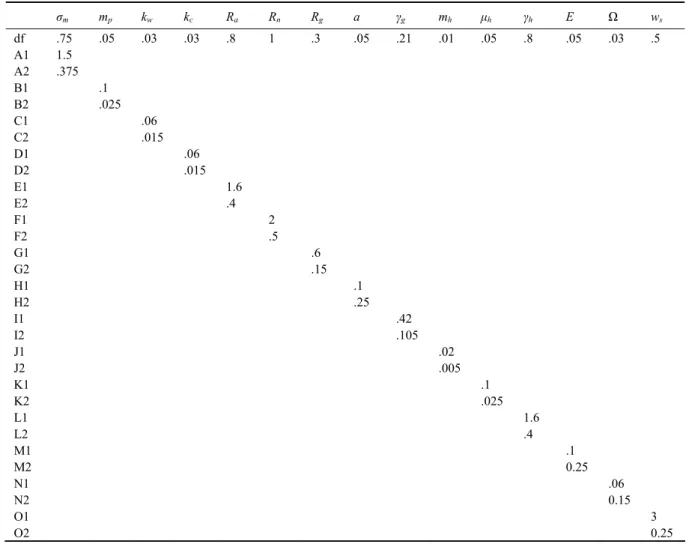
A series of experiments are carried out to analyze the model sensitivity to some adjustable parameters (Table 1). The experiments and the parameter values for each ex-periment are listed in Table 3. The exex-periments show that if one parameter affects phytoplankton distribution, it will have more influence on zooplankton. The important pa-

rameters that affect the structure of phytoplankton, and therefore that of zooplankton, are the maximum phyto-plankton growth rate σm, the phytoplankton death rate mp,

the light extinction coefficient kw, the nitrate half-

satura-tion constant Rn, the maximum herbivore grazing rate rg,

the herbivore death rate mh, the herbivore excretion rate

μh, the herbivore assimilation efficiency γh, the herbivore

half-saturation constant Rg, the detrital remineralization

rate ε, and the detrital sinking rate ws. The bloom

struc-ture is not sensitive to the phytoplankton self-shading coefficient kc, the ammonium half-saturation constant Ra,

the photosynthesis efficiency parameter a, and the am-monium oxidation rate. Three examples are presented below to examine how the biological parameters affect phytoplankton and zooplankton.

Table 3 Parameters for sensitivity experiments (‘df’ stands for the default value. The default is used if no value is shown in a box)

σm mp kw kc Ra Rn Rg a γg mh μh γh Ε Ω ws df .75 .05 .03 .03 .8 1 .3 .05 .21 .01 .05 .8 .05 .03 .5 A1 1.5 A2 .375 B1 .1 B2 .025 C1 .06 C2 .015 D1 .06 D2 .015 E1 1.6 E2 .4 F1 2 F2 .5 G1 .6 G2 .15 H1 .1 H2 .25 I1 .42 I2 .105 J1 .02 J2 .005 K1 .1 K2 .025 L1 1.6 L2 .4 M1 .1 M2 0.25 N1 .06 N2 0.15 O1 3 O2 0.25

5.1 Sensitivity to the Extinction Coefficient of PAR Value (Default kw=0.03m−1)

As shown in Table 3, two experiments were carried out with the PAR extinction coefficient of kw=0.06m−1 and

kw=0.015m−1 in experiments C1 and C2, respectively.

Increasing the default kw value intensifies the distribution

of phytoplankton and zooplankton towards the sea surface (Figs.10c and 10d). Decreasing its value, the distributions of phytoplankton and zooplankton are stretched into deeper water (Figs.11c and 11d). In the model, the

phyto-plankton growth rate depends on the minimum of nutrient limitation and light limitation. It is governed by the ni-trogen limitation near the surface and by the light limita-tion at deeper levels. Comparing the light limitalimita-tion in Fig.10a with Fig.6a, it can be seen that the light limitation in experiment Cl decreases in the entire water column except for the very near surface. The most striking dif-ference is that in the default case, the 0.05 contour of light limitation is located between 100 and 150m depths, while it is between 66 and 84m in experiment Cl. The subsur-face maxima of net limitation decreases and shifts

to-wards the sea surface except in winter, which corresponds to the squeezing of the phytoplankton distribution to-wards the sea surface. The zooplankton, which feeds on

phytoplankton, also moves about 50m closer to the sea surface than in the default case. The dynamics in experi-ment C2 is opposite to that in experiexperi-ment Cl.

Fig.10 The time and depth variations in Expriment Cl of a) the light limitation function, b) the net limitation function, c) phytoplankton, and d) zooplankton in one year.

Fig.11 The time and depth variations in Expriment C2 of a) the light limitation function, b) the net limitation function, c) phytoplankton, and d) zooplankton in one year.

5.2 Sensitivity to the Nitrate Half Saturation Coefficient (Default Rn=1mmolNm−3)

If algae are placed in a nutrient medium, the concentra-tion of nutrients decreases over time in the medium as

they are incorporated into plant cells. The nutrient uptake rate of algae depends on nutrient concentration in the me-dium (Valiela, 1995). The nitrate or ammonium uptake rate of phytoplankton has a hyperbolic relationship with the nitrate or ammonium concentration in the

environ-ment (Eppley et al., 1969). In the Michaelis-Menten equation, the half saturation constant reflects the relative ability of phytoplankton in using nutrients of low levels and thus may be of ecological significance. In the case of nitrate, nutrient uptake occurs in two steps. First, nutrients are taken into a phytoplankton cell at a rate determined by ambient nutrient concentration. Then, as the concentra-tion inside the cell increases, nutrient is utilized in pro-portion to internal cellular concentration. If the nitrate uptake rate is measured when ammonium is present, the uptake of nitrate maybe greatly underestimated because of the preference for ammonium by different algae. The half saturation constant is high in more euphotic and nu-trient-rich waters, but is low in oligotrophic waters.

Two experiments were carried out with Rn=2mmolNm−3

and Rn=0.5mmolNm−3 in experiments Fl and F2,

respec-tively. Increasing Rn in expriment Fl increases the

strength and duration of the phytoplankton spring bloom (Figs.12a and 12b). The subsurface maximum of phyto-plankton now extends into July, while in the default case it extends into June. However, zooplankton has only weak distribution that spans the period from July to No-vember in the upper 120m. Opposite results were ob-tained when the value of Rn was decreased in case F2

(Figs.12c and 12d). The subsurface maximum of phyto-plankton now only extends into May while the distribu-tion of zooplankton is much stronger than in experiment F1, spanning the period form March to November.

Fig.12 The time and depth variations of a) phytoplankton and b) zooplankton in case Fl; c) phytoplankton and d) zooplankton in case F2.

5.3 Sensitivity to the Detrital Sinking Rate (Default ws=0.5md−1)

The sinking rate of particulate organic matter, ws, is

one of the most critical parameters in the model. The ap-propriate value of ws for the model is 0.5md−1, which

implies that the faster sinking and larger particles do not contribute to the processes taking place within the eu-photic zone. Greater sinking values of detrital material decrease the detritus and subsequently nitrogen concen-trations in the euphotic layer. Figs.13a and 13b show the results with the sinking rate of 3md−1_{, and Figs.13c and}

13d 0.025md−1_{. The change in w}

s alters the whole

bio-logical system drastically. In case O1, ws=3md−1, and

there exists only a weak bloom in April and May (Fig.13a), with almost no zooplankton biomass and detri-tus in the study area. The euphotic layer is depleted of both ammonium and nitrate accumulated at deeper levels. The case with ws=0.025md−1 allows a more than

com-plete remineralization of detrital material before it reaches the lower boundary of the model. The concentrations of phytoplankton and zooplankton are higher with the de-crease of ws, than in the default case as shown in Figs.13c

and 13d, especially during winter when the complete wa-ter column overturning provides rich supplies of nutrients in the euphotic zone.

6 Conclusions

In this paper, the interaction between physical and bio-logical dynamics in the Sargasso Sea is studied. The re-sponse of a five-component ecosystem to the external forcing, including heat flux, wind, and salinity, and sensi-tivities of the ecosystem to biochemical parameters are investigated.

The model results compare quite successfully with the observations and the calculated results by Doney et al. (1996). The base simulation and the sensitivity experi-

Fig.13 The time and depth variations of a) phytoplankton and b) zooplankton in case O1; c) phytoplankton and d) zooplankton in case O2.

ments show a seasonal cycle of physics and biology. In summer, the shallow seasonal thermocline depth and the weak convection inhibit nutrient supplies from the mixed layer below, therefore the concentrations of all bio-chemical variables are low and limited to a thin surface layer. In winter, the strong vertical mixing and convection bring more nutrients to the euphotic zone. Hence, in March and April, right after winter, phytoplankton feed-ing upon nutrients reaches its sprfeed-ing bloom level. The bloom of zooplankton, which feeds on phytoplankton, follows the bloom of phytoplankton with a time lag of about two weeks. The results of the sensitivity experi-ments show that zooplankton is generally more sensitive to the variation of biochemical parameters than phyto-plankton. The system is sensitive to all the parameters except the phytoplankton self-shading coefficient, the ammonium half-saturation constant, the photosynthesis efficiency parameter, and the ammonium oxidation rate. For example, a smaller detrital sinking rate and a higher detrital remineralization rate provide higher nutrient con-centration in the euphotic zone, while a smaller light ex-tinction coefficient corresponds to stronger and deeper penetrating solar radiation in water column. Both circum-stances create a more intense bloom, deeper in space and lasting longer in time.

Acknowledgements

We thank Prof. Temel Oguz at the Institute of Marine Sciences, Middle East Technical University, Turkey, and Prof. Xianqing Lv at Ocean University of China for helpful discussions. This work was supported by the Shandong Young Scientists Research Awards under grant

BS2011HZ021.

References

Blumberg, A. F., and Mellor, G. L., 1987. A description of a three-dimensional coastal ocean circulation model. In: Three Dimensional Coastal Ocean Models. Heaps, N. S., ed., American Geophysical Union, Washington, DC, 1-16. Collins, A. K., Allen, S. E., and Pawlowicz, R., 2009. The role

of wind in determining the timing of the spring bloom in the Strait of Georgia. Canadian Journal of Fisheries and Aquatic Sciences, 66 (9): 1597-1616.

Denman, K. L., and Pena, M. A., 2002. The response of two coupled one-dimensional mixed layer/planktonic ecosystem models to climate change in the NE subarctic Pacific Ocean. Deep-Sea Research II, 49 (24-25): 5739-5757, DOI: 10.1016/ S0967-0645(02)00212-6.

Doney, S. C., Glover, D. M., and Najjar, R. G., 1996. A new coupled, one-dimensional biological-physical model for the upper ocean: Applications to the JGOFS Bermuda Atlantic Time Series (BATS) Site. Deep-Sea Research II, 43 (2-3): 591-624.

Eppley, R. W., Rogers, J. N., and McCarthy, J., 1969. Half-saturation constant for uptake of nitrate and ammonium by marine phytoplankton. Limnology and Oceanography, 14: 912-920.

Eppley, R. W., 1972. Temperature and phytoplankton growth in the sea. Fishery Bulletin, 70: 1063-1085.

Esbensen, S. K., and Kushnir, Y., 1981. The heat budget of the global ocean: An atlas based on estimates from surface ma-rine observations. Climatic Research Institute, Report 29, Oregon State University, USA.

Fasham, M. J. R., Ducklow, H. W., and McKelvie, S. M., 1990. A nitrogen-based model of plankton dynamics in the oceanic mixed layer. Journal of Marine Research, 48: 591-639.

Hurtt, G. C., and Armstrong, R. A., 1996. A pelagic ecosystem model calibrated with BATS data. Deep-Sea Research II, 43: 653-683.

Isemer, H., and Hasse, L., 1985. The Bunker Climate Atlas of the North Atlantic Ocean: Volume 2: Air-Sea Interactions. Springer-Verlag, New York, 252pp.

Jassby, A. D., and Platt, T., 1976. Mathematical formulation of the relationship between photosynthesis and light for phyto-pankton. Limnology and Oceanography, 21: 540-547. Knap, A. H., Michaels, A. F., Dow, R. L., Johnson, R. J.,

Gun-dersen, K., Sorensen, J. C., Close, A. R., Hammer, M., Bates, N., Knauer, G. A., Lohrenz, S. E., Asper, V. A., Thel, M., Duddow, H., and Quinby, H., 1993. Data Report for BATS 25-BATS 36, October 1990–September 1991. U. S. JGOFS Bermuda Atlantic Time-series Study, U. S. JGOFS Planning Office, Woods Hole, MA, 339pp.

Knap, A. H., Michaels, A. F., Dow, R. L., Johnson, R. J., Gun-dersen, K., Sorensen, J. C., Close, A. R., Hammer, M., Knauer, G. A., Lohrenz, S. E., Asper, V. A., Thel, M., Dud-dow, H., Quinby, H., Brewer, P., and Bidigare, R., 1992. Data Report for BATS 13-BATS 24, October 1989–September 1990. U. S. JGOFS Bermuda Atlantic Time-series Study, U. S. JGOFS Planning Office, Woods Hole, MA, 345pp. Knap, A. H., Michaels, A. F., Dow, R. L., Johnson, R. J.,

Gun-dersen, K., Knauer, C. A., Lohrenz, S. E., Asper, V. A., Tuel, M., Duddow, H., Quinby, H., and Brewer, P., 1991. Data Report for BATS 1-BATS 12, October 1988–September 1989. U. S. JGOFS Bermuda Atlantic Time-series Study, U. S. JGOFS Planning Office, Woods Hole, MA, 286pp.

Mann, K. H., and Lazier, J. R. N., 1991. Dynamics of Marine Ecosystem Biological-Physical Interaction in the Oceans. Blackwell Scientific Publications, 466pp.

Mellor, G. L., 1990. User’s Guide for a Three Dimensional, Primitive Equation Numerical Ocean Model. Princeton Uni-versity, Princeton, NJ, 35pp.

Mellor, G. L., and Yamada, T., 1982. Development of a turbu-lence closure model for geophysical fluid problems. Reviews of Geophysics and Space Physics, 20 (4): 851-875.

McClain, C. R., Esaias, W. E., Feldman, G. C., Elrod, J., Endres, D., Fireston, J., Darzi, M., Evans, R., and Brown, J., 1990. Physical and biological processes in the North Atlantic during the first GARP global experiment. Journal of Geophysical Research, 95: 18027-18048.

Menzel, D. W., and Ryther, J. H., 1960. The annual cycle of primary production in the Sargasso Sea off Bermuda. Deep-Sea Research, 6: 351-367.

Mitchell, B. G., Brody, E. A., Holm-Hansen, O., McClain, C., and Bishop, J., 1991. Light limitation of phytoplankton bio-mass and macronutrient utilization. Limnology and Ocean-ography, 36: 16662-1677.

Musgrave, D. L., Chou, J., and Jenkins, W. J., 1988. Application of a model of upper-ocean physics for studying seasonal cy-cles of oxygen. Journal of Geophysical Research, 93: 15679-15700.

Oguz, T., Ducklow, H., Malanotte-Rizzoli, P., Tugrul, S., Nezlin, N., and Unluata, U., 1996. Simulation of plankton productivity cycle in the Black Sea by a one-dimensional physical-biological model. Journal of Geophysical Research,

101 (C7): 16585-16599.

Radach, G., and Moll, A., 1993. Estimation of the variability of production by simulating annual cycles of phytoplankton in the central North Sea. Progress in Oceanography, 31: 339-419.

Sharples, J., and Tett, P., 1994. Modeling the effect of physical variability on the midwater chlorophyll maximum. Journal of Marine Research, 52: 219-238.

Valiela, I., 1995. Marine Ecological Process. Springer Verlag ed., 686pp.

Varela, R. A., Cruzado, A., Tintore, J., and Ladona, E. G., 1992. Modeling the deep-chlorophyll maximum: A coupled physi-cal-biological approach. Journal of Marine Research, 50: 441-463.

Warren, S. G., Halm, C. J., London, J., Chervin, R. M., and Jenne, R. L., 1988. Global distribution of total cloud and cloud type over the ocean. NCAR Technical Note, NCAR-TN 317.

WHOI, and BBSR, 1988. Woods Hole Oceanographic Institu-tion and Bermuda Biological StaInstitu-tion for Research, StaInstitu-tion ‘S’ off Bermuda, physical measurements 1954–1984. WHOI and BBSR Data Report, MA, 189pp.

Wroblewski, J. S., Sarmiento, J. L., and Flireal, G. R., 1988. An ocean basin scale model of plankton dynamics in the North Atlantic 1. Solutions for the climatological oceanographic con-ditions in May. Global Biogeochemical Cycles, 2: 199-218. Wroblewski, J., 1977. A model of phytoplankton bloom

forma-tion during variable Oregon upwelling, Journal of Marine Research, 35: 357-394.

Zhu, J., Kamachi, M., and Wang, D. X., 2002. Estimation of air-sea heat flux from ocean measurements: An ill-posed problem. Journal of Geophysical Research, 107 (C10), DOI: 10.1029/2001JC000995.