Digital audio filter design using frequency transformations

Digital Audio Filter Design

Using Frequency Transformations

Chalee Asavathiratham

Submitted to the Department of Electrical Engineering and Computer Science

in Partial Fulfillment of the Requirements for the Degrees of Bachelor of Science in Electrical Engineering and Computer Science and Master of Engineering in Electrical Engineering and Computer Science

at the

MASSACHUSETTS INSTITUTE OF TECHNOLOGY May 23, 1996

@ Massachusetts Institute of Technology 1996. All rights reserved.

Author ...

Department of Electrical Engineering and Computer Science May 23, 1996

C ertified by ...

7!

Alan V.

Oppenheim

Dist*pguished roessor of Electrical Engineering

' D' !

t!

a

A ccepted by... .. ... ... .. ... ... ... Frederic R. Morgenthaler cqairman, Department 1 C mmittee on Graduate Students

MASS ,CHUSETTS INSTITUTE

Digital Audio Filter Design

Using Frequency Transformations

by

Chalee Asavathiratham

Submitted to the Department of Electrical Engineering and Computer Science on May 23, 1996, in partial fulfillment of the

requirements for the degree of

Bachelor of Science in Electrical Engineering and Computer Science and

Master of Engineering in Electrical Engineering and Computer Science

Abstract

This thesis involves designing discrete-time filters for modifying the spectrum of audio signals. The main contribution of this research is the significant reduction in the order of the filters. To achieve this, we have combined a technique called frequency transformation, or frequency warping, with an effective Finite Impulse Response (FIR) filter design algorithm. Both techniques exploit some properties of audio filters which allow us to relax the design specifications according to human auditory perception.

We show several properties of frequency transformations and explain their importance in designing audio filters. We incorporate this technique into design procedures and test them with sample filters. We study the signal flowgraphs of warped filters and evaluate their computational requirements and performance in the presence of quantization noise.

Thesis supervisor: Alan V. Oppenheim

Acknowledgments

I am very grateful to Dr. Paul Beckmann of Bose Corporation, whose guidance, and encouragement have been a tremendous help for me to finish this thesis. It was simply a privilege for me to work with him. I am also very thankful to Professor Alan Oppenheim for giving me the opportunity to work on this problem, for teaching me everything about signal processing, and for taking me into the Digital Signal Processing Group, where I get to meet with wonderful new friends. My gratitude also extends to the Bose Corporation whose generosity has supported this research for the past one and a half years.

Finally, I would like to thank my family and friends for the all their love and support.

Contents

1. Introduction 8

2. Audio Filter Specification and Design 11

2.1 Logarithmic Frequency and Magnitude Specifications ... 12

2.2 Insignificance of Phase Response ... ... 13

2.3 Sample Frequency Responses ... ... 14

2.4 Just Noticeable Difference Curves ... 17

2.5 Limitations of Standard FIR and IIR techniques ... 21

3. Frequency Transformations 22 3.1 Allpass Transformation ... 22

3.2 Properties of Allpass Transformations ... 27

3.2.1 Order Preserving... 28

3.2.2 Allpass Property Preserving ... ... 28

3.2.3 Minimum-phase Preserving ... ... 31

3.3 Design Procedure with Frequency Transformations ... 35

3.3.1 Summary of Design Steps... 35

3.4 Choosing A Warping Factor... 40

4. Polynomial Fitting within Upper and Lower Bounds 45 4.1 Parks-McClellan (Remez) Algorithm ... ... 47

4.1.1 Automatic Order Increase... 49

4.2.1 Conditions on the Minimal Order of the Solutions ... 53

4.2.2 Description of the Algorithm ... 53

4.2.3 Solution Polynomials: p, and p ... ... 54

4.3 Comparisons on Practical Issues... ... 54

4.4 Precision Requirements in Filter Design ... 55

5. Results From Filter Design Experiments 56 5.1 Filter Orders and Comparison with Remez Algorithm ... 56

5.2 Experimentally Obtained Optimal Warping Factors ... 63

6. Implementation Issues 66 6.1 Quantization Noise Analysis in Fixed-Point Arithmetic... 66

6.1.1 Warped Direct-Form FIR Implementation ... .67

6.1.2 Warped, Transposed, Direct-Form FIR Implementation ... 72

6.2 Memory and Computations Requirement... ... 75

7. Conclusions and Suggestions for Further Research 78

List of Figures

Figure 2-1 (a)-(d) Examples of Frequency Response Specifications ... 16

Figure 2-2 Filter used in obtaining the Just Noticeable Difference Curve. ... 19

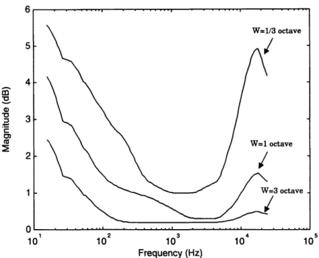
Figure 2-3 JND curves for W=1/3 octave, 1 octave and 3 octave. ... 19

Figure 3-1 Derivation of G(z- 1) based on a substitution of variables in H(z-') ... 24

Figure 3-2 W arped frequencies ... 26

Figure 3-3 Typical target Frequency ... ... 35

Figure 3-4 JND bounds ... 36

Figure 3-5 Warped target response Hd(Oa(e-~ )) ... 37

Figure 3-6 FIR filter design results ... ... 38

Figure 3-7 Effective frequency response of the final system ... .. 39

Figure 3-8 Summary of Design steps ... 40

Figure 3-9 Relation between the minimal filter order and the warping factor... 42

Figure 4-1 U(x) and L(x) on the interval [-1,1] ... 49

Figure 5-1 (a)-(d) Sample design results. ... ... 61

Figure 6-1 (a)-(b) Direct Form FIR and the warped version... . 68

Figure 6-2 Warped, Direct Form FIR with noise source ... 68

Figure 6-3 Warped, Direct Form FIR with noise sources combined... 70

Figure 6-4 (a)-(b) Transposed Direct Form FIR and the warped version... 73

Figure 6-5 Warped, Transposed Direct Form FIR with noise sources. ... 73

List of Tables

Table 5-1 M inim al orders of FIR filters ... 62

Table 5-2 Experimentally obtained warping factors ... 64 Table 6-1 Computation requirements... ... 76

Chapter 1

Introduction

This thesis deals with the design of discrete-time filters for modifying the spectrum of audio signals. The main contribution of this research is the significant reduction in the memory and computational requirements of the filters. To achieve this, we have combined a technique called frequency transformation, or frequency warping, with an effective Finite Impulse Response (FIR) filter design algorithm.

Frequency transformation is a technique which allows us to produce a filter whose frequency response, G(e'ý'), is equal to that of another filter, H(e'"), except that the frequency axis is rescaled. The ability to design a filter on a rescaled frequency axis suits the problem of audio equalization very properly. Since human ears have better frequency resolution at lower frequency than at higher frequency, filter design algorithms must pay attention to the fine details in the low frequencies. As the low-frequency details becomes finer, the required filter length becomes longer. By exploiting the relationship between the frequency response H(ej') and the frequency-transformed response G(e'), we can design a short-length FIR filter h[n] and choose a transformation such that G(ei') has not only the desired audio equalization, but also a low order like that of h[n]. Note that due to the frequency transformation, the filter G(eiJ) will be IIR (Infinite Impulse Response) even though

h[n] is FIR. Thus, we are able to draw on the wealth of FIR filter design algorithms and use them to design IIR filters.

Further reduction in filter length is achieved by designing FIR filters based on a model of human audio perception. Specifically, the deviation in the response of a filter from the desired one is weighted against a perceptual bound. This bound represents the threshold at which a typical listener can detect an error in the frequency response. This model allows us to relax the FIR filter design constraint, from designing a filter that must precisely fit a desired response to designing a filter that must lie within upper and lower magnitude bounds.

The two FIR filter design algorithms which we used were the well-known Parks-McClellan algorithm and the lesser-known CONRIP algorithm. Traditionally, the Parks-McClellan algorithm has been widely used to design lowpass and bandpass filters. Here we will use it to fit an arbitrary curve with a weighting function derived from our perceptual model. Though largely overlooked, the CONRIP algorithm suits our application very appropriately and returns the shortest possible FIR filter that fits our error model. However, experimental results in Chapter 5 showed that these two algorithms yield the same minimal order almost all the time. Both of these design algorithms required high numeric precision and failed to converge when standard double-precision arithmetic was used. To overcome this problem, we wrote a library of arbitrary precision mathematical functions and used them during filter design.

Chapter 2 presents an overview of audio equalizer design including frequency magnitude specifications and error bands based on psychoacoustic measures. This section also discusses the problems encountered when standard FIR and IIR filter design methods are used to design audio equalizers. Chapter 3 reviews the idea of allpass transformations and proves several important properties that they possess. It also summarizes the design steps involved in applying frequency transformations. Chapter 4 discusses the Parks-McClellan and CONRIP design algorithms with emphasis on CONRIP. Chapter 5 presents results from filter design experiments and Chapter 6 investigates the noise performance when implementing (not designing) frequency warped filter using finite precision arithmetic. Chapter 7 summarizes the main results of the thesis and suggests directions for future works.

Chapter 2

Audio Filter Specification and

Design

Digital filters can be used in a wide variety of ways to modify audio signals. These modifications can be grouped into three main categories: spectral, temporal, and spatial. Spectral changes are perceived as changes in the frequency response of the audio signal. Temporal changes are perceived in the time domain and examples include echoes and reverberation. Spatial changes modify the perceived location of a sound. All of these audio signal modifications can be achieved through digital filters - digital linear time-invariant systems - and thus there may not always be a clear distinction between them. For example, a digital filter designed for spectral modifications may also cause some perceptible time-domain distortion.

In this thesis, we focus on designing digital filters for spectrally modifying an audio signal. This is probably the most common use of an audio filter and there are many applications. The simplest application is the implementation of tone controls (bass, mid-range, treble) commonly found on audio equipment. Another application might be to compensate for errors in the frequency response of a loudspeaker which result from shortcomings in the transducer. A further application is to compensate for the

constrained speaker position in an automobile or for the damping of the response due to the car interior.

In many cases, we want to be able to change the frequency response in the field, rather than in the factory. In order to accomplish this, the filter design algorithm must be able to operate without supervision. That is, we need a algorithm that is robust enough to return the optimal filter without human intervention once inputs are specified.

In this chapter, we discuss specific features of audio equalizers which affect their design and implementation. It will be shown that most traditional IIR design techniques and FIR implementations are not suitable for use in audio equalizers.

2.1 Logarithmic Frequency and Magnitude Specifications

Experiments have shown that the human auditory system has better resolution at low frequencies than at high frequencies [1]. For example, it is quite easy to distinguish between 100 and 110 Hz, but extremely difficult to distinguish between 10000 and 10010 Hz. Due to this property, audio equalizers require much higher resolution at low frequencies than at high frequencies. A good model which approximates this behavior is to assume that the frequency specifications are uniform when viewed on a logarithmic frequency scale.

Frequency specifications on a log scale are given in fixed multiplicative increments. One standard unit of such increments is an octave. A k-octave specification is the

one whose frequency response is given on the set of frequencies fo, 2k fo, 22k f0, ₂3k f₀, and so on. For example, a one-third octave specification shall contain the frequency

response at the following frequencies: fo, 21/3 fo, 22/3 f0, 2fo, etc.

The auditory system can also perceive signals over an enormous dynamic range; from a pin drop to a jet plane. The most appropriate manner in which to represent this range of loudness is in decibels (dB) which is defined as 20 loglo(x). dB is also the standard scale to use when discussing changes in magnitude such as in a

frequency response.

Loudness is also perceived on a dB scale. For example, increasing a signal level from 10 to 20 dB roughly doubles its perceived loudness. Doubling again from 20 to 40 dB doubles it again.

2.2 Insignificance of Phase Response

The specifications of an audio filter are usually given in terms of its magnitude response. For the most part, the human ear is insensitive to small variations in phase, and there is quite a bit of flexibility in selecting the phase response of a filter. Phase only becomes an issue when it is perceived as a time-domain effect such as a delay, early or late echoes, or significant smearing of the audio signal caused by uneven group delays across the frequencies. One way to minimize the audible effect of uneven group delays is to restrict the maximum group delay of the filter. This can be accomplished by designing the audio filter to be minimum-phase.

To achieve minimum-phase, the technique of spectral factorization can be included into the filter design procedure. As each filter design algorithm in this thesis returns FIR filters with linear-phase, we can spectrally factor the output into maximum- and minimum-phase parts. Spectral factorization reduces the order an FIR filter into roughly half. For FIR filters with zeros on the unit circle, certain manipulations need to be performed on the input before the factoring. These procedures are described in detail by Schussler [10, pg. 468].

Since spectral factorization reduces the magnitude of both parts to only the square root of the specification, we must compensate by squaring the magnitude of the specifications before designing the target filter.

2.3 Sample Frequency Responses

The filter design algorithm presented in this thesis was tested using a set of 20 prototypical frequency responses. Several of these responses are shown in Figure 2-1 (a) through (d).

10 10 Co 5 a, m-a -5 -t1 - it. 2 3 4 5 10 10 10 10 10 Frequency (Hz) (a) 10 10 5 -- Q-C S0 -5 -10f 2 3 4 5 10 10 10 10 10 Frequency (Hz) (b) 1_ .. r . ... I · · · ·. · ` -- ' · · I · · · 1 '

""~--5 -10 -1r 10 2 · · · 3··· · · · 4 _ _ __ 10 10 10 Frequency (Hz) 105 (c) 10 10210 10410 10 Frequency (Hz) (d)

Figure 2-1 (a)-(d) Examples of Frequency Response Specifications

-10 _ ______ · · · _____ · · · · ·. ·. 1 · · · · · ~~· ... 1 · · · I ... 1 · . · · · ·

The responses were designed to model the equalization needed to flatten a speaker's measured frequency response in typical listening environments. These responses have a frequency resolution of 1/3 octave. That is, the details of the frequency response are spaced at roughly 1/3 octave.

This data is based on measurements made at Bose Corporation for a variety of speakers and listening environments, and represents averages over many positions within the same room. The target responses are a reasonable test of the performance of a filter design algorithm. Designing filters to actual measured data would produce similar results.

2.4 Just Noticeable Difference Curves

In order to optimally approximate the target frequency responses by a digital filter, we must have some error measure. Standard error measures which are frequently used, such as mean squared error, are inappropriate in this case, because they do not take into account the behavior of the auditory system.

We will take a slightly different approach to approximating the desired response. Due to limitations in the auditory system, the human ear is insensitive to small changes in frequency response. Thus, there is a whole set of filters which sounds indistinguishable from the desired filter. Our goal is to define this set and identify a filter which lies within.

The sensitivity of the human auditory system can be described using Just-Noticeable Differences, or JNDs. The JND for loudness is a frequency dependent

frequency (Hz)

Figure 2-2 Frequency response of the filter used in obtaining the Just Noticeable Difference Curve.

The user is asked if the two signals presented were distinct or indistinguishable. The results of the experiment depend upon the details of the shelf filter: center frequency fc, bandwidth W in octaves, and gain h.

The standard method of probing the limits of the auditory system is to keep f, and W fixed, and then vary the gain h until the signals are "just noticeably different." The center frequency is changed, and the experiment repeated. This produces a curve which is a function of frequency and represents the level in dB at which the listener can detect a W-octave change in level. These curves are plotted in Figure quantity. It has been experimentally determined through a set of subject-based listening tests [1] .

The listening tests proceed as follows. The listener is first presented with pink noise, and then with the same noise filtered by the shelf filter shown in Figure 2-2.

O

10

2.... 3.... 4.... ...

10 10 10

Frequency (Hz)

Figure 2-3 JND curves for W=1/3 octave, 1 octave and 3 octave.

As can be seen, the auditory system is most sensitive to frequencies between 2 and 5 kHz. Also, the larger W, the easier it is for subjects to detect differences.

Unfortunately, these results are difficult to apply to the problem of determining general constraints on a filter such that it sounds indistinguishable from another. Recall that the results are for a single perturbation of width W, and do not apply to simultaneous perturbations at multiple frequencies. In fact, no results from psychoacoustics have immediate application to our problem.

W=1/3 octave

W=1 octave ~ "'~" ' ' '""" ' """" ' ' ""~

2-3 for W=1/3 octave, 1 octave, and 3 octaves, and represent results averaged over many subjects.

We will extend the results for loudness JND in a manner similar to that used to extend audio masking data [1]. An audio signal A can mask another signal B if it is sufficiently loud in level and close in frequency to B. Experiments were conducted for the case of a single sinusoid A masking a bandpass noise B. These results were

then extended - without serious experimental evidence - to the case of multiple

sinusoids masking multiple noises. It was shown that as long as the original masking criterion is obeyed at every frequency, the collection of sinusoids appropriately masks the collection of noises. This principle has been widely applied in the design of audio coders.

We will make a similar assumption in this thesis. For example, suppose that we choose the 1-octave JND curve. Given a desired frequency response, we derive upper and lower bounds by adding and subtracting (in dB) the JND curve. We will assume that any filter which falls completely between the upper and lower curves is

audibly indistinguishable from the desired response.

There is one clear difficulty with this assumption. Suppose that the designed filter falls within the upper and lower bounds of the 1-octave JND curve. However, instead of having a response close to our desired curve which is vertically centered within the bounds, the designed filter has a response which is close to, say, the upper bound for most of the frequencies. Then this means that the width (in frequency) of the deviation from desired response can be wider than one octave. For example, suppose that this "ripple" is 2.5 octaves wide. In order to be inaudible, the height of this ripple must satisfy the tighter 3-octave JND bound instead of the 1-octave bound. There is no way to avoid this a priori. Instead, after the filter has

been designed, we will verify that the width of its ripples satisfy the 1-octave JND curve. Experimentally, we have found that this is always satisfied.

2.5 Limitations of Standard FIR and IIR techniques

There are several shortcomings of designing FIR filters to specifications on a broad frequency range. As specifications are given on log scales, the high density of the details in the low frequency region cause the FIR filter to be too long and too costly to implement. Moreover, the large order of the resulting filters require high-precision arithmetic operations in the design algorithm. Standard double high-precision would be insufficient so that the design algorithm would not converge at all. FFT-based algorithm such as overlap-add or overlap-save may be employed to reduce the computational complexity. Since these algorithms are block-based, they introduce substantial latency which may be inappropriate for some real-time applications.

The problem of existing IIR design techniques is that they cannot handle the required detail of the frequencies response. They often fail to converge to an acceptable solution and require constant supervision from the filter designer as IIR design procedures are usually not completely autonomous.

Chapter 3

Frequency Transformations

This chapter introduces the mathematical definition of a frequency transformation as well as some of its properties. To date, the technique of applying frequency transformations in audio filter design has not been used extensively, although the transformation has been recognized for over 20 years by Oppenheim and Johnson [2]. Classically, this technique was used in the design of filters. We will use it both in the design of filters and in their implementation. As a result, we are able to reduce filter lengths by a significant amount, typically by a factor of 80 or so. Results from filter designs using frequency transformation are summarized in Chapter 5.

3.1 Allpass Transformation

A frequency transformation or frequency warping in its most general sense is any

mapping E of the z-plane, i.e., ®(z- 1) maps the complex plane to itself. A filter g[n] is a frequency transformed version of another filter h[n] if their z-transforms are related by a substitution of variables, or

G(z -1) = H( E(z- 1)).+ (3.1)

+ In this chapter, we choose to write "®(z-_{') is a rational function of z}- "' instead, of "E(z) is a rational function of z" because the former sentence provides us with more

We will refer to h[n] as the prototype filter and g[n] as the transformed or warped filter.

We are only interested in frequency transformations that satisfy the following properties:

1. ®(z- 1) is a rational function of z- 1. 2. E(z-1) maps the unit circle to itself.

3. O(z-1) maps the interior of the unit circle to itself.

The first constraint ensures that the function G(z-1) is a rational transform if H(z-1) is rational. This is important because only filters with rational transforms may be realized. The second constraint ensures that the frequency response G(e-j '_{) of the}

transformed filter is related to H(e-j' ) through a warping of the frequency axis. One way to visualize the response G(e-j_{") is to think of the frequency response H(e}-j •_{) but}

with the frequency axis rescaled, so that the co-axis is "stretched out" in some region and "squeezed in" in some other. The third constraints ensures that G(z-1) will, be stable provided that H(z-_{1) is, because all the poles will stay inside the unit circle}

with the warping.

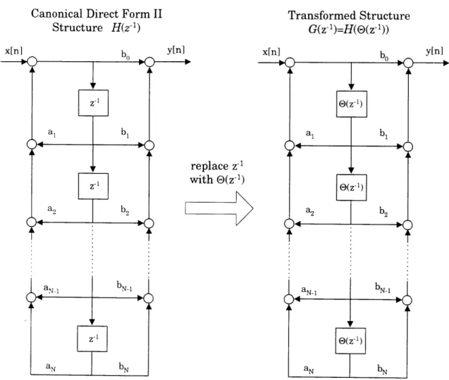
A new idea developed in this thesis is to use the frequency transformation not only in the design phase, but also in the implementation of a filter. Just as the

understanding of the physical implementation; it states that we can substitute every delay with another filter ®(z-1).

transformed and prototype filters are related by a substitution of variables,

G(z-') = H(O(z-1)), the system structure for G(z- 1) can be derived by a direct

substitution of

z-1 --+ (z-1) (3.2)

into the system structure for H(z-1). This is illustrated in Figure 3-1.

Canonical Direct Form II

Structure H(z-1) Transformed Structure_{G(z-1)=H(E(z-1))}

y[n]

replace z-1 with

E(z

Figure 3-1 Derivation of G(z- 1_{) based on a substitution of variables in H(z-').}

It has been shown in [3, pg. 432] and [4] that the most general form of O(z-1_{) that}

satisfies the above three properties is

N -1

6(z-1) -= z -ak foria,k<1.

(3.3)

1 1-akz

In other words, ®(z- 1_{) is a cascade of first-order allpass filters.}

We can constrain the choice of ®(z-1_{) by requiring that the mapping from H(e}-_{j") to}

G(e-j') be one-to-one. Otherwise, G(e-J') would contain multiple compressed copies of

H(e-j") and would greatly limit the types of frequency responses which can be obtained. The constraint that

E(z

transformations to first-order, real allpass functions

-1 =a(z-

) -a where a is real and lal<l1. (3.4) 1- az-1

We will call this type of transformation an allpass transformation. Since, by choice, this transformation maps the unit circle to itself, we can relate a frequency 0 of the

prototype filter with a frequency w of the warped filter by

Se j -a

e - for real 6, 0, a and a < 1. (3.5)

1- ae-j•

from which it follows that

o = arctan[ (1 - a 2_{) sin}

1

[2a +(1+ a2) cos 0(

or equivalently,

S= w + 2 arctan acosin (3.7)

Notice that the function Oa(z-1

) is bijective and its inverse is simply another allpass

(3.8)

(3.9)

For rational filters, G(z-1) can be obtained from H(z-1_{) by replacing every delay wivth}

an allpass filter. The parameter a in ®(z- 1) is called the warping factor. It is a free

parameter and gives us some control between the warping from H(e-_{J") to G(e-J"). An}

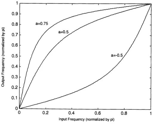
example of the function a(e-j") for a few values of a is plotted below.

1 0.9 0.8 0.7 0.6 0.5 0.4 0.3 0.2 0.1 0 0.2 0.4 0.6 0.8 1

Input Frequency (normalized by pi)

Figure 3-2 Frequencies warped by Allpass frequency transformations with different parameters.

-1

1 + az -1

=Oa(z-1).

To summarize, a function G(z-') is a frequency transformation of H(z-_{') if}

G(z-1) = H( a (z-'))

-1a

=H(

For 0 < a < 1, the effect of the allpass transformation is to stretch the low frequencies of H(e-i') and compress the high frequencies. Similarly, for -1 < a < 0, the low frequencies are compressed and the high frequencies stretched.

This stretching and compressing of the frequency axis is the key benefit of frequency warping and yields a substantial reduction in filter order.

As discussed earlier, an audio filter is often specified on a logarithmic scale due to human auditory perception. If we plot out a typical response specification on a linear scale, we would find that the filter detail is very dense in the low-frequency region, and sparse (or monotonic) in the high-frequency. It is conjectured that the narrow features of the frequency response down in the low-frequency range are the main cause for long FIR filters. An intuitive understanding of this conjecture can be obtained by considering the design of a bandpass filter. The narrower the passband we require, the longer the FIR filter will be. Since an arbitrary audio filter can be approximated as many passband filters connected in parallel, the minimum order of an FIR filter that meets the requirement is dictated by the narrowest passband. Hence, by applying a frequency transformation, we hope to increase the width of the narrow features of the frequency response and thereby decrease the overall order of the filter. This conjecture has been confirmed experimentally with the filter design results in Chapter 5.

3.2 Properties of Allpass Transformations

In this section, we show several properties of allpass transformation which are of interest to audio applications. We will assume that h[n] is an FIR filter with

z-transform H(z-1). The filter G(z- 1) is defined to be the allpass frequency-transformed (or warped) version of H(z- 1) with some warping parameter a as in (3.9).

3.2.1 Order Preserving

Suppose that the FIR filter h[n] has N+1 filter coefficients, or equivalently, N zeros.

Then after allpass transformation, the warped filter G(z- 1) = H(9a(z-1_{)) shall be a}

rational IIR filter, with N zeros and N poles. Moreover, all the poles occur at a, the warping factor. This property can shown by direct substitution,

H(z - 1) = h[0] + h[1]z- 1 + h[2]z- 2 +... + h[N]z-N -1 G(z- 1 ) = H ( -a ) 1- az-1 z - 1 -a 2 -1 N (3.10) = h[O] + h[1] + h[2] +... + h[N] 1 - az- azaz h[0] + h[1]z- 1 + h[2]z- 2 + ... + h[N]z- N (1- az- 1)N

Thus, although allpass transformations changes the filter from FIR to IIR, it preserves its order.

3.2.2 Allpass Property Preserving

It is surprising that if H(z-_{') is an allpass filter, then G(z}- 1_{) will be an allpass filter}

too, since the allpass transformation maps the unit circle to itself. However, for completeness, we have included a proof here.

The most general form of an allpass filter H(z- 1_{) is}

Mr _{z-1 - dk m -_ e)(z}1 _{- ek)}

H(zk) = (3.11)

where the dk's are the real poles and the ek's are the complex poles of H(z-').

Then by warping the filter H(z-') with parameter a, we get

-1 G(z-l ) = H( Z -a 1 - az-1 Mr _ - dk M - ekJ-1 - - ek (3.12)

=r 1-az-1

kII

_-1

1

To help manipulate the complicated expressions in (3.12), we consider the effect of warping on the real and the complex sections separately. For each real section with

a pole at dk, the warped filter can be reduced to

-1 z -a 1-az 1 - dk z-1 (1 + adk)- (a + dk) - z - 1 _{- a (1+adk)-(a} + dk)z -1 1- az1 (3.13) -1 a +dk z 1+adk 1-a + dk -1 1+ad_k

Similarly, each section corresponding to complex-conjugate poles ek and e* can be reduced to

z -a z -a

-az 1-az z - (1+ae )-(a+ek) z-'(l+ae)-(a+ek)

z-1 -a z - 1 -a (1+aek)-(a+ek )z-1 (lae)-(a + e;)z- 1

1ek1 - e k OZ

1 - az- _{1 -}

az--1 a + ekz- 1 a + ek

1+ ae 1+ aek 1 + ae 1 + ae( 3 1 4)

1 + a

--

(3.14)

1+aek 1- a+ek Z- 1 l+aek 1 a+ek -1

1+ aek 1+ aek -1 a + ek -1 a + ek z z 1 + aek _{1+ aek} 1 a+ek -1 a+ek -1 1 z 1-1 aek k+ _{1+ aek}

Substituting (3.13) and (3.14) into (3.12), the warped filter G(z- 1_{) can be expressed}

as Mr -1 M -1 -1 G(z-1) = -rkk (3.15) k=1 rk-1 H -1)(1 - S1 k--1 k= 1 SO- sk -where a+dk r_k 1 + adk a + ek 8 k - -1+ aek

are the new sets of poles. Since the form of G(z- 1) in (3.15) is that of an allpass filter, we conclude that allpass transformations preserve the allpass property of a filter.

The allpass preserving property of the allpass transformation is not directly useful for designing audio filters. However, it is useful for the proof of the next property which is much more significant: the minimum-phase preserving property.

3.2.3 Minimum-phase Preserving

The allpass transformation also preserves the minimum-phase property of a filter. Namely, if H(z-') is a minimum-phase filter, then so is the warped version G(z-1). As discussed earlier, this property is important to audio filters because a minimum-phase filter possesses the minimum energy delay property. The easiest way to see why this is true is to notice that the poles and zeros of H(z- 1) which are inside the unit circle will always stay inside after warping. This is because, by choice,

e,(z

must map the interior of the unit circle to itself.

Another intuitive argument of why an allpass transformation preserves the minimum-phase property relies on the invertibility of the allpass transformation Oa(z-1). Given a filter H(z-1), we can factor it into minimum-phase and the allpass components as shown

H(z -1_{) = Hap(Z}-1

) - Hmin(Z-1). (3.16)

On the other hand, the transformed filter G(z- 1) = H(®a(Z-1)) can also be factored in the same way,

G(z- 1) = Ga(z- 1) - Gmi(z-1). (3.17)

Since we have already shown that the transformation preserves the allpass property, Gap(Z-1

) must contain the transformation of Hap(Z'), which is an allpass filter, plus possibly some extra allpass filter Kap(-1). That is,

Conversely, since ®(z-1) is invertible, we can transform Gap(z- ) by ®0,-(z-1) to obtain

another allpass filter. Moreover, Gap(Oa -)) z-1 must be included in Hap(z-_{') because,}

by definition, Hap(z- 1_{) encompasses the entire allpass portion of H(z-1).}

Thus,

Hap(z

where Cap(z-1_{) is any extra term that HW(z}-1_{) might contain. Then by replacing every}

z-lin (3.19) with ea(z-1

), we have a transformation of HaP(z-) again.

Hap(a(z- 1_{)) = Gap(z}-1₎

Cap(Oa(-1)) (3.20)

This implies that Hap(O(z-1_{)) contains at least every term of}

Gap(Z-1). However,

(3.18) also says that Gap(Z- 1

) contains at least every term of Hap(O(z-1)). Therefore,

Gap(z-1) = Hap(a(Z-1)) (3.21)

which implies that

Gmin(Z- 1) = Hmin( Oa(z-1)). (3.22)

A more formal proof is done by showing that each singularity (pole and zero) of G(z-') is within the unit circle as long as the corresponding singularity of H(z-_{') is}

within the unit circle. Let us assume H(z-1_{) is a rational, minimum-phase filter}

with complex poles and zeros,

H(z-1) = (1-sz - 1) (1 -s₂z( - l- ) _(3.23)

(1 -p1z -1) (1- p2z-l)

(-pn

Since H(z- 1_{) is minimum-phase, there is an equal number of poles and zeros.} Furthermore, I s I < 1 and I pi I < 1. Let us transform H(z-1_{) with parameter a so}

Each term in the numerator and denominator can be simplified as z- 1 -a - - 1 az- - sz - + sia 1-s i 1- az-1 1 - az-1 1+ sia - (a + si ) z- 1 1 - z- 1

la

1 si

_Z-1

-By substituting expression (3.25) into (3.24), we obtain

G(z-1)

=

With this new expression for G(z-1), the question is whether the new poles and zeros are inside the unit circle. That is, we must show that I c I < 1 as well as I d, I < 1. To see why this is true, let us rewrite the magnitude squared of the numerator of ci as

a + si2 _{= (a+s)(a + )} = a2 + as, + a•, + 2 Si (3.28) = a2+

2aRe{s,}

1-_

az-11 + asi2 = (1+ asi ) (1+ a-i)

= 1+ asi + asi + a2 Si 2 (3.29)

= 1+ 2aRe(si + a2 _{Si 2}

Since 0• la I < 1, and 0: I si I < 1, we can write them as a2 = 1 - for 0 < z 5 1

(3.30)

si,2 =1- a forO<ac1.

By substituting (3.30) into the expression for the numerator ci in (3.28), we get

a + s2 = (1- ) +2aRe(s +(1 -) (3.31)

= 2 + 2aRe(s,

}

Similarly, the denominator of ci in (3.29) becomes

1 + asi 12 = 1 + 2aRe{si } + (1- e)(1- a)

= 2 + 2aRe(si - - a + ca(3.32) (3.32) = a +si + Ea > a + si 2. Therefore, Ga+8 i ci = < 1. (3.33) I1 + as,

By repeating the argument above with si replaced with pi, we can conclude that

IdiJ = a + < 1. (3.34)

l +api

Thus, all of the singularities of G(z- 1_{) are within the unit circle and therefore, G(z}-1₎

is a minimum-phase filter.

3.3 Design Procedure with Frequency Transformations

This section is an overview of the entire design procedure when the frequency transformation technique is used. It also discusses how one chooses a warping factor so that the filter order might be minimized.

3.3.1 Summary of Design Steps

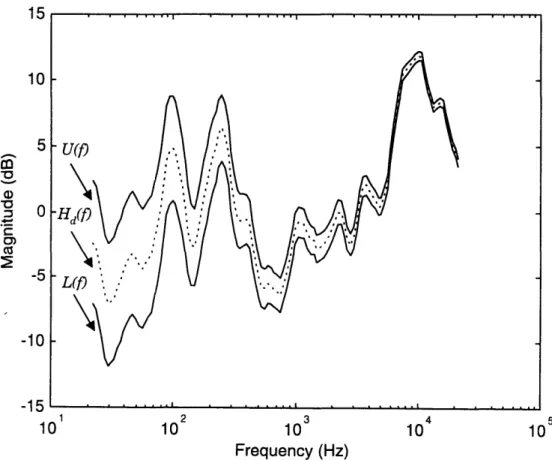
First we are given a target frequency response Hd(f) on a logarithmic scale. We apply the Just-Noticeable Difference (JND) curve to obtain the upper and lower tolerance bounds, U(f) and L(f) as shown below.

10 102 103

Frequency (Hz)

410

10 105

Figure 3-3 A typical target Frequency Response Hd(f) with Just-Noticeable

Difference bounds U(f) and L(f).

_ _ _ ______ _ ____~~~ - * * * * * * * * * * . . . ... . . . .·. • • ,·· • , * * .. . . . . I . . . . . j". 1

-15

0 0.5 1 1.5 2 2.5

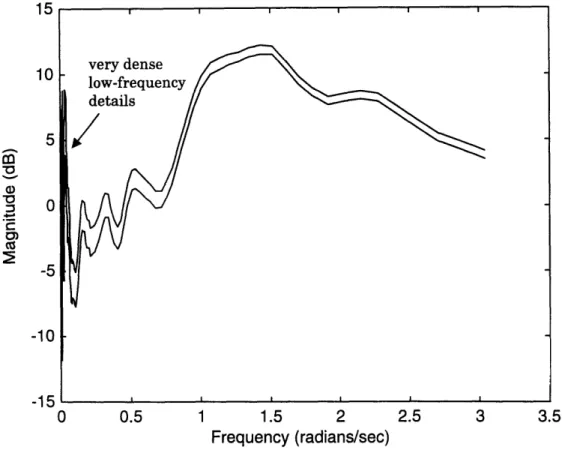
Frequency (radians/sec)

3 3.5

Figure 3-4 JND bounds U(e-j") and L(e-j') plotted on a linear,

sampling-frequency normalized scale.

Next, we use the allpass frequency transformation to "stretch out" the crowded low-frequency region and simultaneously "squeeze in" the high-low-frequency region. How we determine the parameter a in the transformation is explained in the next section. Suppose we choose the warping factor a to be 0.93. The frequency warped

15 10 5 0 -5 -10 -15

Notice that the magnitude specification above is in dB or 20loglo(Magnitude), and that the frequency spans roughly the entire audible range (20 Hz to 20 kHz). On a linear scale normalized by sampling frequency, the upper and lower bounds, U(e~")-j and L(e-j") have a very dense low-frequency specification as shown in Figure 3-4.

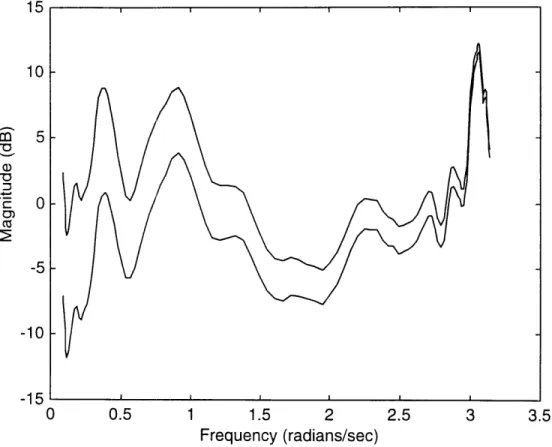
(Oa(e-"J)) now looks much more similar to its original log-scale specification, gure 3-5.

-5

0 0.5 1 1.5 2 2.5 3

Frequency (radians/sec)

Figure 3-5 Warped target response Hd(®a(e-j _)).

set off to design a filter that lies within those error bounds. We choose to an FIR filter instead of IIR because of the availability of many design Is. For this example with a=0.93, the shortest FIR filter has a length of 68 Figure 3-6 below confirms that its magnitude meets our constraints.

-10

-15

3.5

I I I I I I

0 0.5 1 1.5 2 2.5 3 3.5

Frequency (radians/sec)

Figure 3-6 FIR filter design results

To implement the actual filter, we simply build the FIR filter network and inverse-warp it by replacing all the delays with allpass filters with parameter a= -0.93. The final frequency response of the filter implemented using frequency warping is shown below. 38 10 10 5 C, -5 -10

15a

-I

1 2 3 4 5

10 10 10 10 10

Frequency (Hz)

Figure 3-7 Effective frequency response of the final system

As described in section 2.2, in general we can reduce the order of the FIR filter into half by spectrally factoring out the minimum-phase part before the final warping. However, since spectral factorizations reduce the magnitude of filter to only its square root, we must compensate by squaring the magnitude of the input upper and lower bounds before the first warping. The entire design procedure is summarized into the following diagram.

10 10 -5 -10

-r

Figure 3-8 Summary of Design steps.

3.4 Choosing A Warping Factor

As mentioned earlier, it is only a conjecture that the frequency warping technique is beneficial to digital filter design when the desired response is given on a logarithmic

Specification

scale. We made no attempt in proving it. Nor did we mathematically characterize the "shape" of the frequency response that would yield the low filter order. However, experiments have shown such positive results (savings of nearly two orders of magnitude in filter order) that we believe it is a rather plausible assumption and we state it loosely here.

Assumption 1 (Even Spread): Given a fixed level of error, the order of the (rational) filter that meets a desired frequency response is lowest when the details of the desired response are spread out, or warped, as evenly as possible in frequency. This is when considering the response on a linear frequency scale.

The next question is naturally in the choice of the allpass transformation that achieves the above assumption. In other words, we must pick the warping parameter a in the allpass transformation

-1

S(z-1) = -a (3.35)

1- az1

such that the desired frequency response is spread out as evenly as possible when plotted on a linear scale. From Figure 3-1, we know that the optimal value of a must be positive because positive values of a magnify the low-frequency region where the details of a specification are most crowded. We predict that the relation between the values of a (in the range [-1,1]) and the corresponding minimal FIR filter is bitonic in a; the order first decreases monotonically until it reaches a minimum and then increases monotonically, as shown.

0.5 1 a Range of

optimal a

Figure 3-9 Prediction of the relation between the minimal possible filter

order and the warping factor.

From the figure, it is worth noticing that the because the filter order is discrete, the plot exhibits a stair-like shape. Secondly, because slight variations in a need not change the order of the filter, the optimal warping parameter is not single-valued, but lies in a range of values.

In practice, it would be much more convenient to have an a priori estimate of the optimal warping factor instead of searching by trial-and-error for all a between 0 and 1. In order to obtain a closed-form solution for such an estimate, we formulate the problem as follows.

Assume that the desired frequency response takes the form of N+1 piecewise constant, logarithmically spaced bands, called band 0 through band N. Let the

log-scale center (in radians/sec) of the ith band be

Bi = Bor' for 0 < iN and for some r > 1 (3.36) Minimal FIR filter order

where Bo is the log-scale center of the lowest band. r controls the spacing between adjacent bands. For example, suppose that a sample of 44.1 kHz is used, the first band is centered at 25 Hz, and the band spacing is one-third octave, Then

2,r25

Bo - _____5 3.56 x 10- 3 rad / sec (3.37) 44100

and

r = 21/". (3.38)

We will assume the ith band occupies the frequency in the range

[Bir-g,Bir2). (3.39)

Therefore, the width of ith band is

1 1

Wi = Bir - Bir . (3.40)

Define the linear-scale center of the ith band to be the average of the upper and lower boundary, i.e.,

1 1

Ci = (B r + Bir ) . (3.41)

For convenience, we will now replace the notation

ea(e

1 1

Wa.i = Oa(Bir ) -e(Bir 2) . (3.42)

Let the log-optimal warping factor d be the one which maximizes the narrowest band after warping, or more formally,

a = arg max min Wa,i. (3.43)

This minimax problem can be solved numerically using an exhaustive search by a computer. It might seem at first difficult to perform an exhaustive search over the variable a since it is a continuous variable. However, experience has showed that d is usually in the range between 0.8 and 1. This allows us to search through a discretized set of a within a restricted range.

As an example, suppose we design an equalizer for the entire audible frequency range which extends from 20 Hz to 20 kHz. There are 30 bands (band 0 through 29) and each band is spaced apart at one-third octave (r=2113_{). The first log-scale band}

center is fixed at 25 Hz. Assuming that the sampling rate is at 44.1 kHz, then by a searching through the values of a discretized to multiples of 0.001, we find that

Chapter 4

Polynomial Fitting within Upper

and Lower Bounds

As described earlier, our specification for an audio filter will take the form of two real boundary functions, the upper and lower bound. We look for filters whose magnitude responses are vertically bounded by those two functions, and have a maximum ripple width less than some fixed bandwidth.

Our design procedure is as follows. First, we ignore the second requirement about the maximum ripple width for a moment, and only search for filters that fall within the prescribed magnitude bounds. We will call this the Constrained Ripple problem. Then, after obtaining such filters, we will verify that they also satisfy the ripple width constraint. This chapter concerns only the first part: designing filters that fit within the upper and lower bounds.

We will concentrate only on Type I filters. That is, a filter h[n] with an odd length M+1 that satisfies h[n]=h[M-n]. From Oppenheim and Schafer [3, pg. 465], a type I linear-phase FIR filter can be transformed to a polynomial, and vice versa. By applying this polynomial transformation to the upper and lower bounds, we effectively get two polynomials in the range [-1,1]. We will refer to the upper and lower bound as U(x) and L(x) respectively. Our job now is to find a polynomial that

lies in between these polynomials. Therefore, our discussion in this chapter will only be based on a polynomial in the variable x. Once we find that polynomial, we can inverse-transform it back to an FIR filter and then warp h[n] to obtain the audio

equalizer g[n].

In this chapter, we describe two design algorithms which return such polynomials: Parks-McClellan and CONRIP. We will emphasize the lesser known algorithm discovered by M. T. McCallig [5], [6]. The algorithm CONRIP (CONstrained RIPple) iteratively finds a polynomial that meets the upper and lower bound constraints. Moreover, the algorithm guarantees that the polynomials found has the minimum possible length of all valid polynomials.

We chose not to analyze the performance of the windowing design method, because this method cannot be performed without supervision. In Parks-McClellan and CONRIP, the algorithms always perform a solution search as exhaustively as they can for each given filter order. If the algorithms fail to find a solution, the only way to proceed is to keep increasing the order until a solution is found. On the other hand, when a windowing design method fails for a given filter order, it is unknown whether the correct approach is to increase the filter order or to modify the target response. This is due to the lack of direction in choosing the target frequency response, which is allowed to lie anywhere within the vertical bounds. Certainly, we may take an arbitrary approach in increasing the order every time windowing fails, but this will yield a solution with unnecessarily large order.

4.1 Parks-McClellan (Remez) Algorithm

The algorithm of Parks-McClellan [7] adapted the second algorithm of Remez [8, pg. 95] to find a polynomial whose weighted error is minimized. Although Parks-McClellan has been traditionally used in designing filters with piecewise constant or piecewise linear response mixed with don't-care regions, there is nothing intrinsic about the underlying theory that prevents one from designing a polynomial to fit an arbitrary curve. The set of classes of functions to which the Remez exchange algorithm can apply is very broad. Precise necessary conditions on the desired function Hd(x) can be found in [8].

There are only three inputs to the Parks-McClellan algorithm: a filter order, a desired function Hd(x) and a weighting function W(x). The Parks-McClellan algorithm returns the Mth-order polynomial A(x) which minimizes the maximum weighted approximation error. That is, it determines a set of coefficients

{po0,

M

A(x) = pxi, (=4.1)

and for a closed subset Fp consisting of disjoint union of closed subsets of the real axis x, the maximum weighted error

max I W(x)(Hd (x)- A(x)) (4.2)

x Fp

is minimized [3, pg. 468]. Note that the weighting function W(x) does not give us direct control over the absolute sizes of the approximation errors. Rather, W(x) controls the ratio of the ripple sizes. Thus, for a given set of tolerances, it is

necessary to apply the Parks-McClellan iteratively with various filter orders until the specifications are met.

In the audio filter design problem, we are given upper and lower bounds U(x) and L(x) (where U(x) > L(x)), but no desired response Hd(x). In order to adapt the audio filter design problem to use the Parks-McClellan algorithm, we propose using

Hd (x)

=

(U(x)

+ L(x))

(4.3)

and

1

W(x) = (4.4)

Y₂ (U(x) - L(x)

If we apply the Parks-McClellan algorithm on this set of inputs and increment the filter order until the weighted error is less than 1, then we have found a solution to the constrained ripple problem as well. More precisely, if A(x) has a weighted error less than 1 then,

1> W(x)(Hd (x)- A(x)), Vx EF,

Y

(U(x)

+

L(x)) - A(x)

(4.5)

Y (U(x) - L(x))

which makes

Y

(U(x)

-

L(x))

>

Y

₂

(U(x) + L(x))- A(x)

> -

Y

2

(U(x) -L(x)).

(4.6)

This reduces to

A(x) > L(x)

(4.7)

and A(x) < U(x) as desired.

U(x)

1/2 [U(x)- L(x)]

Hdx

-1 0 1

Figure 4-1 Polynomials of upper and lower bound U(x) and L(x) on the

interval [-1,1]. The middle curve Hd(x) is the average magnitude of U(x) and

L(x).

4.1.1 Automatic Order Increase

Another advantage of using the constant 1 as the threshold for rejecting or accepting a design is the ability to detect early on if a given polynomial order is too small. This capability allows the filter designer to increase the order without carrying the algorithm to convergence. The detection can be done as follows. Suppose the Remez algorithm is currently searching for an optimal polynomial at An intuitive argument is as follows. Hd(x) is the middle curve between the two bounds, and W(x) the inverse of one-half of the gap width. So at any point x, if the error is larger than one-half the width of the gap, then it must have exceeded the bound. The conjecture in setting Hd(x) to be the midline allows the resulting polynomial to have as large a vertical "swing" as we can afford, which, in turn, should keep the polynomial order low.

order L. In each iteration, we must compute an approximating polynomial based on a certain set of interpolation points I xi, yi I for 0 • i • L. The algorithm states that the y-coordinate of this set of points must be chosen to be as close to Hd(x) as possible. Specifically, the weighted error between Hd(x) and the interpolating polynomial when evaluated at xo, x1, X2,..., x, must be minimized. Note that this

does not mean that the weighted error evaluated at other points would be minimized as well. By the alternation theorem, this produces a unique polynomial whose weighted error at the points xi are of equal magnitude and alternating sign.:

g,-s, , -s,..., (-1) L+1&

In the proof of convergence of this algorithm, Cheney [8, pg. 98] has shown that the absolute value of the weighted error, 6S , forms a bounded, monotonically increasing sequence with each iteration. This means that we can increment the polynomial order L as soon as S11 > 1, instead of waiting until I15 converges.

Unfortunately, even if we try every order n starting from n=2 as the polynomial order, until the weighted error is less than unity, we still cannot be certain if the filter order we have arrived is the minimum taken over all polynomials which are the solutions to the constrained ripple problem; it is only the minimum order taken from the set of solutions from Remez algorithm when given the above Hd(x) and W(x) as inputs.

4.2 CONRIP algorithm

Although the method above describes a way in which we can arrive at a solution, it does not guarantee that the solution has minimal order. In his thesis [6], McCallig

proved that a filter resulting from his algorithm will always have the minimal length among the valid filters meeting the upper and lower constraints. Also, he showed that if his algorithm fails to find such a polynomial, then no polynomial exists which meets the constraints.

To date, there have been very few references to his thesis. Hence, we would like to reiterate some of the highlights of the theories that he developed. Although some theorems have been proven for generalized polynomials (or Chebyshev Systems), our presentation here is in terms of ordinary polynomials 1, x, 2,..., x" since they are of main interests to us.

Definition (P,): Given continuous functions U(x) and L(x) on [-1,11 such that U(x)

> L(x) for each x, let P, be the set of all polynomials p(x) of order n,

n

p(x) = pix i (4.8)

i=O

such that L(x) < p(x) < U(x) for -1 < x < 1. By the Weierstrass Approximation Theorem [8, pg. 66], P, is non-empty for sufficiently large n.

Before introducing the next definition, it is worthwhile to point out that in order to specify a polynomial of degree n uniquely, we need exactly n+1 coefficients

Po, P1,...,Pn. Alternatively, we can also specify it with n+1 interpolation points

(Xo',Yo), (xi, yO), -.. , (Xn,

y,)

i#j.

Definition (P,): Given U(x) and L(x), let P, be the set of nth-order polynomials

point being on U(x). The abscissas of the interpolation points are arranged in increasing order, i.e., x_o < x₁ < ... < x,.

Definition (Pd): The set P1 has the same definition as Pu except that the first

interpolation point is on L(x).

Note that a polynomial could be in P, and P1. For example, consider a polynomial

g(x) from Pu. At xo, g(xo)=U(xo) by definition. However, in the region where x < Xo, we cannot predict how g(x) behaves. It might cross L(x) at, say, x_. This means we can1

also specify g(x) by interpolating through

(x-_,L(x-1)), (x0,Yo), (x1,Y1), "", (Xn-1,Yn-1)-Therefore, g(x) e Pu n P1.

Theorem 4.1 (Existence of p. and p_): If n is large enough so that Pn is not empty, then

I. P, rn P, contains a single polynomial p+ II. Pn n P1 contains a single polynomial p_

Proof: The proof may be found in [9, pg. 72].

Theorem 4.1 is fundamentally important to CONRIP. It states that if, for a fixed order, there exists any polynomial lying within the bounds at all, then there must also exist two polynomials which touches the upper and lower boundaries

alternately. This is the reason that CONRIP directs all its effort only into searching those two particular polynomials: p+ and p_.

4.2.1 Conditions on the Minimal Order of the Solutions

McCallig also proved the following two theorems which are very useful in determining if a given order n is the minimal order.

Theorem 4.2 (Conditions on n being too small): P, is empty if and only if P,: n

Pt is not empty.

Theorem 4.3 (Conditions on n being too large): The coefficients of the term x"

of p+ and p_ are of opposite signs if and only if the polynomial order n is not minimal.

Proof: The proof can be found in [6].

4.2.2 Description of the Algorithm

As an important part of his thesis, McCallig presented a very efficient algorithm that finds p, and p_. The CONRIP algorithm is strikingly similar to the Remez exchange algorithm. With each passing iteration, the state of the algorithm takes the form of n+1 interpolation points (xi, yi). During each iteration, the interpolation points would produce a unique polynomial, from which we obtain the new set of interpolation points. If n is sufficiently large so that Pn is non-empty, then the algorithm converges to p+, and, with some modification in the algorithm, p_. If n is too small, the algorithm would eventually produce a polynomial which is in P, n Pt.