De-noising and de-blurring of images using deep neural networks
by
Amanda Fike
Submitted to the
MSHUSETS INSTITUTEOF TECHNOLOGY
JUL 16 2019
LIBRARIES
ARCHIVES
Department of Mechanical Engineering
in Partial Fulfillment of the Requirements for the Degree of
Bachelor of Science in Mechanical Engineering
at the
Massachusetts Institute of Technology
June 2019
0 2019 Massachusetts Institute of Technology. All rights reserved.
Signature of Author:
Signature redacted
Signature redacted
Certified
Department of Mechanical Engineering
May 10, 2019
George Barbastathis
Professor of Mechanical Engineering
Thesis Su" erxviscr
De-noising and de-blurring of images using deep neural networks
by
Amanda Fike
Submitted to the Department of Mechanical Engineering
on May 10, 2019 in Partial Fulfillment of the
Requirements for the Degree of
Bachelor of Science in Mechanical Engineering
ABSTRACT
Deep Neural Networks (DNNs) [1] are often used for image reconstruction, but perform better
reconstructing the low frequencies of the image than the high frequencies. This is especially the
case when using noisy images. In this paper, we test using a Learning Synthesis Deep Neural
Network (LS-DNN) [2] in combination with BM3D [3], an off the shelf de-noising tool, to
generate images, attempting to decouple the de-noising and de-blurring steps to reconstruct
noisy, blurry images. Overall, the LS-DNN performed similarly to the DNN trained only with
respect to the ground truth images, and decoupling the de-noising and de-blurring steps
underperformed compared to the results of images de-blurred and de-noised simultaneously with
aDNN.
Thesis Supervisor: George Barbastathis
Title: Professor of Mechanical Engineering
Table of Contents
A b str a ct
...
3
In tro d u ctio n
...
5
F ig u re I ... 5M eth o d s
...
6
F ig u re 2 ... 7 E q u atio n I ... 7 F ig u re 3 ... 8R esu lts
... 8
F ig u re 4 ... 9 F ig u re 5 ... 10 F ig u re 6 ... 10 F ig u re 7 ... I IC o n clu sio n
...
1 1
References
...
12
Introduction
In low light conditions, images end up looking noisy or grainy. This noise applied to the images is Poisson noise, a signal dependent noise. Since the signal is noise dependent it is harder to de-couple from the system. Particularly with Poisson noise, the mean is equal to the variance [4]. This means that the noise to signal ratio is the square root of the mean. That is to say that as the mean (photo
n levels) increases, the image appears less noisy. In Gaussian noise, however, the noise is additive and easier to decouple from the system. In this paper we attempt to decouple the de-noising and de-blurring processes by converting Poisson noise to Gaussian noise, de-noising the image, and finally de-blurring the image. One method that has been used for de-noising images is a program developed by researchers at the Tampere University of Technology called BM3D [5]. Since Poisson noise is more relevant in low photon cases and BM3D works specifically on Gaussian noise, it is important to transform the Poisson noise to Gaussian noise. This can be done with the Anscombe variance stabilization transform (or the
generalized Anscombe variance stabilization transform which takes into account both Poisson and Gaussian noise) [3]. However, this transform is limited in cases of extremely low photon levels.
Deep Neural Networks [1] have been used for some time for image reconstruction. Phase extraction neural networks (PhENN) in particular will be used in this paper [6]. PhENN specifically was developed to retrieve phase information from intensity images, giving depth information. The general architecture of PhENN, a U-Net [7] with skip connections, has been proven to be highly effective in many other applications. Here it is not used to gather information on phase retrieval, but rather to use the same network architecture to de-blur images that are previously de-noised by the BM3D algorithm.
Another common issue with most current image reconstruction algorithms is that lower frequencies tend to be over-represented in the results. Take image de-blurring as an example. In blurry images, the higher frequencies are lost. In order to reconstruct the higher frequencies from the blurry images, the algorithm must rely on the prior knowledge of the image database. Because the database is
sparse in the higher frequencies, the lower frequencies tend to be over-represented in the final images. The nonlinear operations in the DNN only make this worse. In order to address this, Deng and Li proposed a Learning Synthesis Deep Neural Network (LS-DNN) [2]. LS-DNN first takes two DNNs which are trained with respect to low frequencies and with respect to high frequencies separately, generating preliminary reconstructions that are reliable in low and high frequencies respectively. The preliminary reconstructions are then passed on to a third DNN which acts as a learned synthesizer between the high and low frequency reconstructions, resulting in reconstructions that have high fidelities in all frequencies. These are referred to as DNN-L, DNN-H, and DNN-S for high, low, and synthesis respectively throughout the rest of the paper. The structure of the LS-DNN can be seen in Figure 1.
--Skip Connectaoe Down-Resklual Block (DAB) * Upesidua Black (URS) * Dilatd Residu Black PDRO)
Residuall Block (RB)
owl2 I1 I OW .y 0.4 UU&I L 2 !br ll Us
6"68da
64.117
Figure l b
Reeldual Residual
upsamping unit downeampling unIt
(2,2) (2,2) Trumpm B~c A Convoludw 2,) (1,1) (1,13 c o'Cm luion Residual unit (1.1) Convokurn Jli (1,1) suconWluum Up-residual Down-residual u N31
block (URB) block (DRB)
uunk lidr unki
Figue dic
Figure Ilc
Figure 1: a) This show the PhENN (U-Net with skip connections) used in this paper [2]. b) This shows the original PhENN architecture [6]. c) This image shows the structure of the residual/convolution blocks [2].
Methods
This method attempts to decouple the de-noising and the de-blurring processes, using BM3D [3]
for de-noising and LS-DNN [2] for the de-blurring.
To train the neural net, noisy and blurry images first needed to be synthetically generated due to lack of experimental data. Starting with the ImageNet database, images were first blurred and then synthetic noise was applied. For the training set, 10000 images were used and for the testing set, 100 images were used.
First blur was applied to the images using a low pass filter. Level of blurriness could be
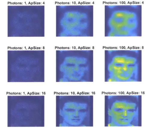
determined by aperture size. Noise was applied using a Poisson noise function in MATLAB. In Figure 2 variety of photon levels and aperture sizes contribute to different levels of noise and blur. For the rest of the testing and training, only one level of blur was used, but the photon levels, corresponding to the mean
of the images, were applied at 1, 5, 10, and 100 photons
LI. 'M
Photons: 10. AoSize: 4 Photons: 100. ApSize: 4
Photons: 1, ApSize: 8 Photons: 10, ApSize: 8 Photons: 100, ApSize: 8
Photons: 1, ApSize: 16 Photons: 10, ApSize: 16 Photons: 100, ApSize: 16
Figure 2: On the horizontal axis there are different levels of noise. The
amount of noise corresponds to illumination levels in the physical world. On the vertical axis there are different levels of blur applied to the picture. The aperture size corresponds to the size aperture the Fourier transform of the image would be passed through to create blur.
Often neural networks approach de-noising and de-blurring in the same step. This approach, however, tries to decouple the two processes. First, the noisy, blurry image needed to be put through BM3D, a standard de-noising software. However, due to the fact that BM3D was made for Gaussian noise, a MATLAB software was used that instead put the image first through an Anscombe variance stabilizing transform given in Equation 1 then through BM3D. This transform was used to make an image contaminated by Poisson noise appear to be an image contaminated by Gaussian noise, making the
BM3D applicable.
x -- 2 x + (1)
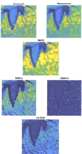
Following that, the image was put through a standard PhENN and in parallel put through a
PhENN where the ground truth images are high frequency pre-modulated. Finally, the results of these
DNNs were put through a final DNN-S, which synthesizes the two preliminary reconstructions into a final image. An example of all the stages is shown in Figure 3.
Ground truth Measurement
BM3D
DNN-L DNN-H
LS-DNN
Figure 3: From the ground truth and measurement to final image, this
image exhibits the chronological order the steps are completed in to reach the final image.
Results
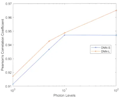
When testing, the LS-DNN [2] was expected to visually outperform the DNN [1] that only took the ground truth image for training. The results showed the latter DNN having a higher correlation to the ground truth image. However, both sets of results have a large degree of variability as seen in Figure 4.
DNN-S] 0.98 DNN-L C 0.96 o 0.94 . 0 0.86 0.84 0.82 100 101 102 Photon Level
Figure 4: This figure shows the Pearson's correlation coefficient for
all 100 test images compared to the ground truth image versus the
photon levels. The error bars show
+/-
one standard deviation.
The DNN-S has lower average Pearson's correlation coefficients than the DNN-L. This,
however, is to be expected, due to fact that the standard DNN trains to maximize the correlation
coefficient between the ground truth and the final image, whereas the LS-DNN attempts to make
images appear visually improved. In Figure 6, however, we can see that this is not the case when
the de-noising and de-blurring steps are de-coupled.
Looking at a single image, Image
35,
we see similar correlation to the mean in Figure
5.
Figure 6 and 7 show these results visually. The DNN-L and DNN-S appear to be performing
similarly. Interestingly, the BM3D seems to produce similar results regardless of the noise level,
as seen in Figure 6. For high photon levels, the images visibly lose high frequency information
from the over-smoothing effect of the BM3D.
'3, 0 0 0 0 0.97 0.96 0.95 0.94 0.93 0.92 0.91 100 101 Photon Levels
Figure
5:
This shows Pearson's correlation coefficient
versus the photon levels used to generate noise. The
correspond well with the means.
Pnimann Nnina BM3D DNN-L 102
of image
35
correlations
DNN.4LliaI
L~A
Figure 6: This image shows Image
35
over increasing photon
levels: 1,
5,
10, 100 from top to bottom and all the resulting images
from the process. There is not visibly much difference in detail
between DNN-L and DNN-S.
DNN-SIA
li
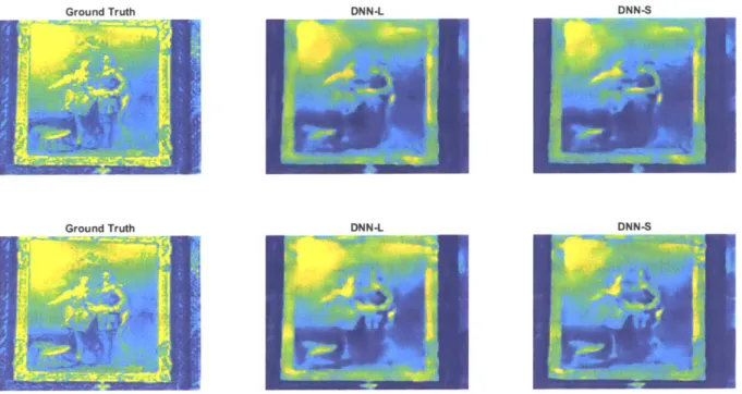
- A DNN--+ -DNN-Ground TruthGround Truth DNN-L DNN-S
Ground Truth DNN-L DNN-S
Figure 7: Here is a closer look at Figure 6's 5 and 10 photon images,
focusing primarily on the DNN-L and DNN-S. The DNN-S seems to have made only a slight difference in the images.
Conclusions
Overall, breaking the process into de-noising by BM3D [3] followed by de-blurring by DNN [1] was not as effective as training it exclusively on a DNN. The time implications of the BM3D were heavy: each image took about half a second to put through the Anscombe transform and the BM3D. In addition, the BM3D caused an over-smoothing effect. While the de-noised image looked better than the
measurement, the process caused the image to lose some of its information. This was both true of high and low photon cases. In the case of high photon, there is visibly information lost from the BM3D process. Finally, due to the high frequencies lost with the over-smoothing, the LS-DNN [2] performed worse than the DNN that had not been synthesized by correlation coefficient values, although both experience large variations. Visually, LS-DNN performed similarly to the DNN trained on solely the ground truth.
Since the BM3D was likely the cause of much of the over-smoothing and information loss, future work should avoid relying heavily on this algorithm while also using a DNN.
References
[1] Y. LeCun, Y. Bengio and G. Hinton, "Deep learning," Nature, vol. 521, pp. 436-444, 2015.
[2] M. Deng, S. Li and G. Barbastathis, "Learn to synthesize: splitting and recombining low and
high spatial frequencies for image recovery," arXiv, 2018.
[3] M. Maggiano, E. Sanchez-Monge, A. Foi, A. Danielyan, K. Dabov, V. Katkovnik and K.
Egiazarian, "Image denoising by sparse 3D transform-domain," 2007. [Online]. Available:
http://www.cs.tut.fi/-foi/GCF-BM3D/. [Accessed 12 February 2019].
[4] MathWorks, "Poisson Distribution," The MathWorks, Inc., [Online]. Available:
https://www.mathworks.com/help/stats/poisson-distribution.html. [Accessed 20 April 2019].
[5] M. Maggiano, E. Sanchez-Monge, A. Foi, A. Danielyan, K. Dabov, V. Katkovnik and K.
Egiazarian, "Image and video denoising by sparse 3D transform-domain collaborative
filtering," IEEE Transactions on Image Processing, vol. 18, no. 8, 2007.