HAL Id: hal-00903460
https://hal.archives-ouvertes.fr/hal-00903460
Submitted on 21 Aug 2020
HAL is a multi-disciplinary open access
archive for the deposit and dissemination of sci-entific research documents, whether they are pub-lished or not. The documents may come from teaching and research institutions in France or abroad, or from public or private research centers.
L’archive ouverte pluridisciplinaire HAL, est destinée au dépôt et à la diffusion de documents scientifiques de niveau recherche, publiés ou non, émanant des établissements d’enseignement et de recherche français ou étrangers, des laboratoires publics ou privés.
Earthquake synchrony and clustering on Fucino faults
(Central Italy) as revealed from in situ Cl-36 exposure
dating
Lucilla Benedetti, Isabelle Manighetti, Yves Gaudemer, Robert Finkel,
Jacques Malavieille, Khemrak Pou, Maurice Arnold, Georges Aumaitre, Didier
Bourles, Karim Keddadouche
To cite this version:
Lucilla Benedetti, Isabelle Manighetti, Yves Gaudemer, Robert Finkel, Jacques Malavieille, et al.. Earthquake synchrony and clustering on Fucino faults (Central Italy) as revealed from in situ Cl-36 exposure dating. Journal of Geophysical Research : Solid Earth, American Geophysical Union, 2013, 118 (9), pp.4948-4974. �10.1002/jgrb.50299�. �hal-00903460�
Earthquake synchrony and clustering on Fucino faults (Central Italy)
as revealed from in situ
36Cl exposure dating
Lucilla Benedetti,1Isabelle Manighetti,2Yves Gaudemer,3Robert Finkel,1,4 Jacques Malavieille,5Khemrak Pou,1Maurice Arnold,1Georges Aumaître,1 Didier Bourlès,1and Karim Keddadouche1
Received 27 December 2012; revised 15 July 2013; accepted 16 July 2013; published 6 September 2013.
[1] We recover the Holocene earthquake history of seven seismogenic normal faults in the
Fucino system, central Italy. We collected 800 samples from the well-preserved limestone scarps of the faults and modeled their36Cl concentrations to derive their seismic
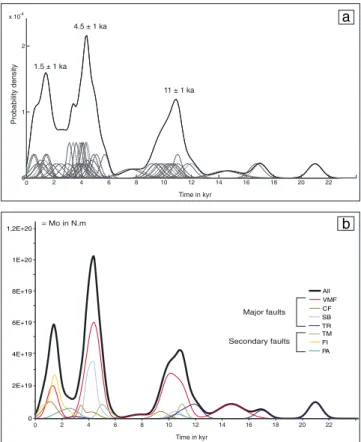
exhumation history. We found that> 30 large earthquakes broke the faults in synchrony over the last 12 ka. The seven faults released strain at the same periods of time, 12–9 ka, 5–3 ka, and 1.5–1 ka. On all faults, the strain accumulation and release occurred in 3–6 ka supercycles, each included a 3–5 ka phase of slow (≤ 0.5–2 mm/yr) strain accumulation in relative quiescence, followed by a cluster of three to four large earthquakes or earthquake sequences that released most of the strain in< 1–2 ka. The large earthquakes repeated every 0.5 ± 0.3 ka during the paroxysmal phases and every 4.3 ± 0.9 ka between those phases. Earthquakes on the northern faults produced twice larger surface slips (~ 2 m) and had larger magnitudes (Mw 6.2–6.7) than those on the southern faults. On most faults, the relative strain level was found to control the amount of slip and the time of occurrence of the next large earthquake. Faults entered a phase of clustered activity once they had reached a specific relative strain threshold. The Tre Monti fault is identified as the most prone to break over the next century. Our data document earthquake synchrony and clustering at a broader space and time scale than has been reported to date.
Citation: Benedetti, L., I. Manighetti, Y. Gaudemer, R. Finkel, J. Malavieille, K. Pou, M. Arnold, G. Aumaıˆtre, D. Bourle`s, and K. Keddadouche (2013), Earthquake synchrony and clustering on Fucino faults (Central Italy) as revealed from in situ 36Cl exposure dating, J. Geophys. Res. Solid Earth, 118, 4948–4974, doi:10.1002/jgrb.50299.
1. Introduction
[2] On any active fault, earthquake geology seeks to know: When is the next large (Mw≥ 6–7 depending on the region) earthquake due, where will it occur, and what will be its size? Answering these questions is necessary to assess seismic hazard, as to understand the physics of faults and earthquakes and the rheology of crust and lithosphere. Unfortunately, we are generally unable to answer the above questions. A major
reason is that information that precisely describes the distri-bution of large earthquake occurrence times and slips on a fault is lacking. Instrumental and historical earthquake data provide information on periods that are generally much shorter than the mean recurrence times of large events on faults. Paleoseismological data provide longer records of large earthquakes, but these records are generally still too short to unequivocally document the shape of the distribution of large earthquake occurrence times and slips. Paleoseismological data allow, however, to test the various theoretical models of earthquake occurrence that are pro-posed. These models are of two types [e.g., Kagan and Jackson, 1991; Sornette and Knopoff, 1997; Faenza et al., 2004]. Thefirst type of model is Poissonian, which assumes that a large earthquake occurs on a fault with no memory of the previous event; large events on faults should thus show a memoryless and hence variable distribution of time intervals and slips [e.g., Sornette and Knopoff, 1997 and references therein]. The second type of model assumes the opposite hypothesis in which the occurrence of a large earthquake on a fault depends, at least partly, on the time of the previous large event. The fundamental support for such time-dependent models is the elastic rebound theory [Reid, 1910]. According to this theory, large earthquakes should repeat on a fault at quasi-periodic times and produce
Additional supporting information may be found in the online version of this article.
1
Aix-Marseille Université, CEREGE CNRS-IRD UMR 34, Aix en Provence, France.
2
GEOAZUR, CNRS, IRD, Observatoire de la Côte d’Azur, Université de Nice Sophia Antipolis, Sophia Antipolis, France.
3
IPGP, Équipe de Tectonique, Sorbonne Paris Cité, Univeversity Paris Diderot, UMR 7154, CNRS, Paris, France.
4
Now at Earth and Planetary Science Department, University of California, Berkeley, California, USA.
5
Géosciences Montpellier UMR CNRS 5243, Université Montpellier Place E. Bataillon, Montpellier, France.
Corresponding author: L. C. Benedetti, Aix-Marseille Université CEREGE CNRS-IRD UMR 34, Plateau de l’Arbois, Aix en Provence, 13545, France. (benedetti@cerege.fr)
©2013. American Geophysical Union. All Rights Reserved. 2169-9313/13/10.1002/jgrb.50299
fairly similar slips (so-called “characteristic earthquake model” [e.g., Schwartz and Coppersmith, 1994]).
[3] Although available worldwide earthquake data, includ-ing paleoseismological data, allow testinclud-ing these various models, they do not allow yet to discriminate them. On some fault cases, large earthquakes are found to repeat at fairly reg-ular times and produce similar slip amplitudes [McCann et al., 1979; Shimazaki and Nakata, 1980; Schwartz and Coppersmith, 1994; Nishenko and Buland, 1987; Wesnousky, 1994; Sieh, 1984, 1996; Tapponnier et al., 2001; Haibing et al., 2005; Parsons, 2008; Scharer et al., 2010, 2011; Klinger et al., 2011]. These characteristic earth-quakes are also suggested to break similar sections of the faults. Yet, in many other fault cases, large earthquakes are found to occur in clusters. A cluster is a group of large earth-quakes that occur in a time span considerably shorter than the mean recurrence interval [e.g., McCalpin and Nishenko, 1996]. Earthquake clustering is observed at different time-and space-scales, from< tens of years (e.g., aftershocks se-quences [Kagan and Jackson, 1991] and cascade of events on a fault [e.g., Bernard and Zollo, 1989; Amato et al., 1998]) to centuries [Goes, 1996; Pirazzoli et al., 1996; Stiros, 2001; Stein et al., 1997] and millenniums [Wallace, 1987; Grant and Sieh, 1994; Marco et al., 1996; McCalpin and Nishenko, 1996; Rockwell et al., 2000; Holbrook et al., 2006; Ferry et al., 2007, 2011; Dolan et al., 2007; Sieh et al., 2008; Meltzner et al., 2010; Schlagenhauf et al., 2011], on individual faults, and on different faults within a large-scale fault system [e.g., Bucknam et al., 1980; Baljinnyam et al., 1993; Nur and Cline, 2000; Rockwell et al., 2000; Bell et al., 2004; Vanneste et al., 2006; Scholz, 2010]. When multiple faults within a system are found to break in fairly coeval large earthquakes, the clustering is re-ferred to as earthquake synchrony [e.g., Scholz, 2010]. The increasing number of earthquake data worldwide which doc-ument clustering of strong events makes a number of authors to suggest that clustering and synchrony of large earthquakes are the way most seismogenic faults release the accumulated stresses and strain [Allen, 1975; Wallace, 1987; Kagan and Jackson, 1991; Rockwell et al., 2000; Scholz, 2010]. However, although the longest available earthquake records are up to 20–50 ka long, they might still be too short to rep-resent a statistically meaningful reprep-resentation of the event time and slip distribution. One possibility thus exists that the observed periodicity or clustering of large earthquakes is an artifact within a strictly Poissonian distribution [e.g., McCalpin and Nishenko, 1996; Kagan et al., 2012].
[4] The question of how large earthquakes repeat on faults, and within fault systems, is thus still posed and begging more data to test the available models. In the present paper, we pro-vide new paleoseismological data that document the large earthquake record on seven seismogenic faults. The faults be-long to the Lazio-Abruzzo normal fault network (LAFN) in central Italy, which has been the site of two historical dra-matic earthquakes, the 1915 Avezzano Ms ~ 7 (30,000 casu-alties [e.g., Boschi et al., 1997]) and the 2009 L’Aquila Mw 6.3 (~350 casualties and current allegation of scientists [Chiarabba et al., 2009]) earthquakes. The LAFN includes more than 20 large seismogenic normal faults (i.e., with length≥ ~ 10 km), and we analyze here seven of them that form a ~ 30 km × 100 km large system (Fucino fault system). We collected more than 800 samples in the preserved,
seismically exhumed limestone fault scarps, and measured their content of in situ cosmogenically produced36Cl. The methodology based on the use of the36Cl cosmogenic iso-tope allows measuring the ages and the surface slips of the most recent large earthquakes that contributed to the fault scarp exhumations, and hence recovering the Holocene ex-humation history of the faults. We have pioneered the devel-opment and use of this method [Benedetti et al. 2002, 2003; Palumbo et al. 2004; Schlagenhauf et al., 2010, 2011]. This is thefirst time that the36Cl method is applied to such a large number of faults and so doing, to a large-scale fault system. A corollary is that it is also thefirst time that such a large number of samples—about ten times more than any published data—are analyzed for36Cl content measurement. This dense data collection allows us to recover the number, ages, and slips of the most recent large earthquakes on the seven faults and examine whether these various earthquakes had any temporal or spatial organization on the individual faults and within the entire fault system. Wefind that such an organization did exist as more than 30 large earthquakes broke the seven faults in specific intervals over the last ~ 12 ka.
2. Seismotectonics of the Lazio-Abruzzo and Fucino Fault Systems
2.1. The Lazio-Abruzzo Fault Network
[5] The Fucino fault system belongs to the broader Lazio-Abruzzo fault network (LAFN, inset, Figure 1). About 60 km wide and 100 km long, the LAFN is the largest normal fault network in the Apennines. It formed in the Miocene in re-sponse to an extensional regime that followed the compres-sional phase that had generated the prominent carbonate mountains of central Italy [e.g., Bosi, 1975; Benedetti, 1999; Piccardi et al., 1999]. Though some of the LAFN faults have long been recognized [e.g., Bosi, 1975, Piccardi et al., 1999], some have not been sufficiently mapped, and the geometry of the overall fault network has not been de-scribed. Therefore, our first step was to identify and map the LAFN faults, and we did so based on the combined anal-ysis of seven pairs of stereoscopic panchromatic SPOT satel-lite images of 2.5–5 m resolution, numerous aerial photos of about 1 m resolution, topographic digital elevation models (Shuttle Radar Topography Mission and Advanced Spaceborne Thermal Emission and Reflection Radiometer (ASTER) of 90 and 30 m resolution, respectively), geologi-cal maps [Vezzani and Ghisetti, 1998], and extensive field work. It is now well established that most seismogenic faults can be unambiguously recognized from the trace that they imprint in the surface morphology [e.g., Tapponnier and Molnar, 1977; McCalpin and Nishenko, 1996]. In exten-sional settings as that of the LAFN, the main indications of recent fault movements are well-preserved, steep, continuous cumulative escarpments, triangular facets shaping the fault escarpments, existence of small, steep scarplets at the base of the cumulative escarpments, fault traces cutting across re-cent morphological markers [e.g., Wallace, 1977, Armijo et al., 1992]. These characteristic morphological features are observed along most of the LAFN faults, and this allowed us to recognize faults with recent (i.e., late Quaternary) movement, down to faults of km length scale. These faults are presented in Figure 1. We have mapped with thicker
traces the faults that show either the highest and steepest cumulative escarpments or a small fresh scarplet at the base of their cumulative escarpment. In thinner traces are the sec-ondary faults that we suspect to be active though the morphological evidence is less clear. For clarity, we have simplified the names of the faults compared to many provided in the literature [Galadini and Messina, 1994; Giraudi and Frezzotti, 1995; Salvi and Nardi, 1995; Michetti et al., 1996; Pantosti et al., 1996; Giraudi, 1998; Galadini and Galli, 1999, 2000, Galadini et al., 2003; Piccardi et al., 1999; D’Addezio et al., 2001; Cavinato et al., 2002; Galadini et al., 2003; Salvi et al., 2003; Pizzi and Pugliese, 2004].
[6] The Lazio-Abruzzo fault network is made of a large density of NW to NNW trending, normal faults. These faults organize, however, into four principal, roughly parallel, NW striking, SW dipping systems, from west to east: Liri, Fucino, Aterno-Roccapreturo-Barrea (ARB), and Sulmona-Gran Sasso (SGS) systems. The Liri, ARB, and SGS systems are 80–100 km long, narrow, right stepping en echelon fault zones. They strike NW to NNW overall, but all three systems curve counterclockwise at their northern tip and splay into multiple secondary branches, in a horsetail fashion (see, e.g., Manighetti et al. [2001a] for further details on horsetail faulting). This suggests that the NW trending Liri, ARB, and SGS systems might have a left-lateral component of slip in addition to their dominant normal one.
[7] In between the Liri, ARB, and SGS narrow fault systems extends a broader and more complex fault zone, the Fucino fault system. We describe this system in detail in the following section.
[8] The LAFN has developed in between and superimposed on large, ancient thrust systems (green in Figure 1a), and it is likely that at least the major LAFN normal faults root at depth on thrust interfaces [e.g., Pizzi and Galadini, 2009].
[9] The LAFN has accommodated a ~ N20°E extension at a rate of 2–4 mm/yr over the last decade [Hunstad et al., 2003; Nocquet and Calais, 2004; D’Agostino et al., 2001, 2008; Serpelloni et al., 2007], and possibly up to 3–9 mm/ yr over the last 20 ka [Piccardi et al., 1999]. Each of the four major fault systems described above might thus accommo-date 0.5–2 mm/yr of horizontal extension that might convert into 1–4 mm/yr of vertical slip on each system (assuming an average 60° dip) [Vezzani and Ghisetti, 1998].
[10] Several historical earthquakes of magnitudes up to Mw 7.0 have struck the LAFN over the last 700 years (Figure 1) including the 2009 Mw 6.3 L’Aquila earthquake which broke the northern tip of the ARB fault system (Paganica fault [e.g., Chiarabba et al., 2009; Chiaraluce et al., 2011]). The oldest well-recorded earthquake occurred southeast of Rieti in 1349 (I = IX–X), while the strongest and most destructive event struck the Fucino basin in 1915, destroying the city of Avezzano and most surrounding
villages (Avezzano earthquake, 13 January 1915, I ~ XI, Mw ~ 7.0, 30,000 casualties, Figures 1a and 2b) [e.g., Boschi et al., 1997; Gruppo di Lavoro CPTI, 2004].
2.2. The Fucino Fault System
[11] The Fucino fault system has both common and distinct features compared with the Liri, ARB, and SGS systems (Figures 1 and 2). Similar to the other systems, it is a ~ 100 km long fault zone made of NW to NNW striking, SW dipping normal faults. Most of these faults are segmented in a right-stepping fashion, while they splay to the north in oblique secondary branches. In contrast, the Fucino system is much broader than the other systems and includes several parallel principal fault strands. Also, it is divided into two parts, a northern part, the Fucino north (FN), and a southern part, the Fucino south (FS), by a unique fault, the Tre Monti (TM), that is the only one in the entire region to have an ENE trend. The Fucino system is also the only one to enclose a large (~30 km) and deep (~ 1300 m) basin, the Fucino plain [Cavinato et al., 2002].
[12] The“Fucino north” system includes two parallel NNW trending, W dipping major fault zones, the Fucino northwest (FNW) and the Fucino northeast (FNE) (Figure 2a).
[13] The FNW includes a major fault, the Velino-Magnola (VMF, see Schlagenhauf et al., 2011 for more details), connected to several smaller faults. The VMF is NNW trending, ~ 45 km long and divided into four, 10–15 km long, principal fault segments (Magnola, Velino, Val di Malito, and Castiglione). In the north, the VMF is connected to smaller and more easterly striking faults, the major ones are Piano di Rascino (~ 10 km long) and Fiamignano (FI, ~ 15 km long). In the south, the VMF trace curves to the east (Magnola segment). Given 20°NE extension [Piccardi et al., 1999], dominant normal motion is expected on the Magnola and Fiamignano fault segments, while more oblique motion, both normal and left lateral, is expected on the NNW striking fault segments. These expectations are in keeping with the highest cumulative vertical throws mea-sured on the Magnola segment (~800 m [see Schlagenhauf et al., 2011, Figure 1]) and with the prominent height of the Fiamignano cumulative escarpment (~ 450 m, Figure 2c). All in all, the cumulative vertical slip on the FNW fault sys-tem decreases quite regularly from south to north [see Schlagenhauf et al., 2011, Figure 1]. Well-preserved scarplets are mainly observed in the southern half of the FNW, and along the Fiamignano fault (Figure 2a and supporting information Figures E1).
[14] The FNE is a ~ 45 km long, NNW trending fault zone that is divided into six ~ 10 km long, principal fault segments (Ovindoli, Piano di Pezza, Campo Felice, Monte Ocre, Roio, and Monte Petino faults, Figures 1 and 2b) arranged in a right-stepping echelon, among which the Campo Felice fault (CF) is the largest and the one having the clearest and highest
Figure 1. (a) Seismotectonic map of Lazio-Abruzzo fault system. Normal faults are in black. Shaded relief from 90 m pixel Shuttle Radar Topography Mission digital elevation model, illuminated from NE. Historical earthquakes epicenters (Mw≥ 5.9) are from catalog CPTI04 [Gruppo di Lavoro, 2004] covering the period 217 to 2002. Faults that ruptured in 1915 and 2009 earthquakes are underlined in yellow. Major Cenozoic thrusts are indicated in green [Vezzani and Ghisetti, 1998]. Inset: Major active faults in central Italy with extension direction and largest recent earthquakes. (b) Fucino north and Fucino south normal faults systems highlighted in red and orange, respectively. Squares indicate Figures 2a and 2b. Thicker traces indicate major faults and/or faults with clearest evidence of recent activity.
Figure 2. Active normal faults and paleoseismological sites in the (a) Fucino north fault system and (b) Fucino south fault system. Green rectangles show location of trenches and yellow triangles are36Cl sites discussed in text (see text for references). Faults that ruptured in 1915 are underlined in white. (c) Cumulative displacement versus length profiles measured on each studied fault. The profiles were measured on a digital elevation model with a resolution of 20 m provided by website SINAnet (http://www.sinanet. isprambiente.it/it). Note that the cumulative slip-length profile of the VMF can be found in Schlagenhauf et al., 2011. All profiles are shown at same length scale, but vertical scale differs among the plots (for clarity). The TR profile could be measured only on the central and eastern segments of the fault. Toward their ends, some fault traces become more subtle to identify, or they connect to nearby faults. This explains why certain slip profiles show still significant slip values at their ends. Yellow triangles indicate the36Cl sites.
cumulative escarpment. CF is thus the major fault segment in the overall FNE system. Most of the FNE segments have their trace slightly curving counterclockwise in the north and splaying into several smaller, more easterly striking faults. Together these suggest that the FNE has an oblique normal and left-lateral motion on its NNW mean strike, while dominant normal slip is expected on its more NW trending sections. The FNE cumulative escarpments are smaller than those of the FNW faults (Figure 2c, 400–800 m for FNW and ~ 200 m for FNE). Well-preserved scarplets underline most of the FNE faults, and the Piano di Pezza fault clearly offsets late Quaternary sediments [Pantosti et al., 1996] (supporting information Figure E2).
[15] South of the Tre Monti fault, the“Fucino south” system includes two subparallel NW to NNW trending, ~ 40 km long, W dipping major fault zones, the Trasacco fault zone (TR) and the San Sebastiano fault zone (SB) (Figure 2b).
[16] The SB is among the most continuous and longest fault zones of the Fucino south area, and it also has the highest cumulative escarpment (~ 350 m, Figure 2c), with a cumulative vertical throw that decreases from south to north. It is made of three principal fault segments, Monte Marsicano, Terratta, and San Sebastiano, that form a right-stepping echelon along the mean NNW strike of the fault zone. The SB fault trace curves counterclockwise at both its northern and southern tips, and hence terminates in a horsetail fashion. The horsetail is particularly developed in the NW quadrant of the fault zone, where it includes four principal NW trending, 10–20 km long, south dipping normal faults, the Monte Ventrino, Pescina, Parasano, and Serrone faults. The overall geometry of the SB fault zone thus suggests that its slip is both normal and left lateral on its principal NNW strand, while dominant normal motion is expected on its secondary NW trending horsetail faults. San Sebastiano C umulativ e thr o w (m) C umulativ e thr o w (m) Fault length (km) NW SE 300 200 100 0 0 2 4 6 8 10 10 12 14 16 Fiamignano NW SE 500 400 300 200 100 0 0 2 4 Parasano NW SE 80 120 40 0 0 2 4 Trasacco NW SE 300 200 100 0 0 2 4 6 8 Campo Felice NW SE 200 100 0 0 2 4 6 8 Tre Monti Fault length (km) W E 500 400 300 200 100 0 0 2 4 6
Fucino North faults
Fucino South faults
c
These expectations are in keeping with the high escarp-ments of the Monte Ventrino, East Parasano, and East Serrone faults. Furthermore, the cumulative vertical throws of the Parasano and Serrone faults might be greater than observed at the surface as parts of their escarpments are presently hidden under the thick Fucino sediments; the total vertical displacement on the Serrone fault might actually be greater than 1100 m [Cavinato et al., 2002]. A fresh, ~ 9 and 4–5 m high, limestone scarplet underlines the central part of the SB strand and the Parasano secondary fault, respectively.
[17] The Trasacco fault extends over ~35 km long at the other side of the Fucino plain. It strikes NW overall, and shows a sim-ple geometry with three principal, ~ 10 km long, disconnected fault segments. The two southernmost segments have well-expressed cumulative escarpments, whose height decreases overall from south to north. In contrast, the northernmost segment forms no clear topographic escarpment; its existence in the Fucino plain was revealed by its rupturing in the 1915 earthquake (Figure 2b). If the TR fault is similar to the other NW trending faults of the Fucino region, it may have a
Table 1. Available Data Documenting the Past Earthquakes on the FN and FS Faultsa
Ruptured Faultb Earthquake Age Measured Coseismic Slip Remarks on Age and Slip Determination
Monte Ocre (5) 0.6–3.7 ka 0.3–0.5 m Large range of ages because no clear correlation of events between the two trenching sites two events in
0.6–7.6 ka each 0.3–0.5 m
Ovindoli-Pezza (2) < 1 ka ~ 3 m Event seen at three trenches; preearthquake paleosoil dated with several radiocarbon dates; slip well determined from trench reconstruction 3–4 ka ~ 2. 5 m Event seen infive trenches; age constrained by several radiocarbon dates;
slip well estimated from trench reconstruction > 7 ka not constrained Event seen at one trench only; predates a paleosoil dated with few
radiocarbon data.
Serrone (1,3,4) 1915 AD 0.3–0.6 m 1915 event observed in four trenches
< 1.4 ka BP > 0.3 m Age inferred from one radiocarbon date; slip poorly constrained ~ 2.3–2.9 ka not constrained Nofigure in the paper concerning this event; ages are based on one
thermoluminescence date only and archeological considerations 7.1–10.4 ka BP 2–3 m Slip not well constrained; age bounded by two radiocarbon dates Parasano (4) < 4.5 ka ~ 1 m - No rupture attributed to 1915- Age inferred from archeological
remains in upper soil (no absolute dating) three events in
4.5–20 ka not constrained Age inferred from one radiocarbon age Trasacco NW (4) 1915 AD 0.1–0.7 m 1915 event observed in four trenches
< 2 ka 0.2–0.7 m Offset of a Roman Aqueduc
~ 3.5 ka not constrained Event detection based on unconformities between soil levels; No absolute dating but ages inferred from correlation with Fucino basin stratigraphy 8.0–12.7 ka
After 12.0
a
Bold ages are events that are considered well constrained and thus displayed on Figure 5.
bFrom published records based on trenches. Sources are indicated by the number in parentheses: 1, Michetti et al. [1996]; 2, Pantosti et al. [1996];
3, Boschi et al. [1997]; 4, Galadini and Galli [1999, and references therein]; 5, Salvi et al. [2003].
Table 2. Geometrical Characteristics of36Cl Sites
Fault Site ρrock ρcoll α β γ
Scarp Height H (m) Elevation (± 5 m) Latitude Longitude EL_f Stone 2000 EL_mu Stone 2000 Sampling Height (m) Fiamignano FI 2.68 1.5 12° 40° 38° 20 1178m N42.2720 E013.1161 2.597 1.648 7.1 Campo Felice CF 2.66 1.5 30° 55° 45° 17 1595m N42.2283 E013.4437 3.558 1.974 8.8 Magnola MA1a 2.67 1.5 25° 40° 35° 15 1265m N42.1280 E013.4137 2.771 1.711 8.1
Magnola MA2a 2.67 1.5 35° 50° 35° 8.6 1200m N42.1240 E013.4273 2.636 1.662 8.5 Magnola MA3a 2.7 1.5 30° 45° 30° 20 1255m N42.1190 E013.4480 2.750 1.703 10.1 Magnola MA4a 2.64 1.5 30° 42° 30° 7 1300m N42.1184 E013.4613 2.846 1.737 7.0 Velino VEa 2.71 1.5 30° 40° 35° 9.5 1014m N42.1685 E013.3130 2.281 1.531 7.0
Tre Monti TM 2.67 1.5 20° 72° 35° 3.5 970m N42.0650 E013.4627 2.200 1.499 2.7 Trasacco TR 2.64 2.6 25° 65° 25° 4.7 800m N41.9280 E013.5670 1.916 1.386 4.4 Parasano PA 2.64 1.5 25° 55° 40° 4.0 1270m N41.9961 E013.7027 2.777 1.713 3.3 San Sebastiano SB 2.62 1.5 25° 62° 50° 4.5 1214m N41.9466 E013.7618 2.658 1.671 4.5
dominant normal motion. The central segment of the TR fault is underlined by a 5 m high, fresh scarplet.
[18] The northwestern part of the FS system ruptured dur-ing the devastatdur-ing 1915 Avezzano earthquake (Figure 2b). Evidence for surface ruptures were firmly reported on the Serrone, Trasacco (western segment), and Luco dei Marsi faults (Table 1) [Oddone, 1915; Michetti et al., 1996; Galadini and Galli, 1999]. The Avezzano earthquake likely initiated on and mainly broke one of these faults at depth, with this dominant breaking inducing shallow slip distributed on the nearby faults [Galadini and Galli, 1999; see similar case in Jacques et al., 2011]. The total vertical coseismic slip across all traces was estimated to be 1–3 m.
[19] The Tre Monti fault (TM), about 20 km long, southeast dipping, is the only ENE-WSW-oriented fault in the LAFN. It separates the FN and FS systems, in that the major faults of these two systems end near the Tre Monti fault and do not continue beyond its trace. It forms a ~ 450 m high cumulative escarpment. Seismic profiles across the Tre Monti fault suggest that it might have a cumulative throw of ~ 800 m [Cavinato et al., 2002]. In more detail, the TM fault is made of two principal segments extending on either side of the Celano village, and two parallel, smaller, closely spaced faults (Figure 2b). The two major segments have a ~ 5 m high well-preserved scarplet, and the western segment clearly offsets recent lacustrine deposits [Pizzi and Pugliese, 2004].
[20] Most Fucino faults have a cumulative slip versus length profile that is asymmetric and roughly triangular in overall shape (Figure 2c). These specific slip distributions have been shown to typify faults that are both active and propagating laterally in the direction of slip decrease [Manighetti et al., 2001a, 2001b, 2009; Schlagenhauf et al., 2008]. We infer that the VMF [Schlagenhauf et al., 2011, Figure 1], SB, and PA faults are propagating northward (over multiple seismic cycles, see discussion in Manighetti et al., 2005], while the FI and CF faults are propagating southward. The TM fault has a more elliptical slip profile and hence might not be propagating laterally [Manighetti et al., 2001a, 2001b; Schlagenhauf et al., 2008].
[21] To summarize, the Fucino fault system includes four major faults, two in the north, VMF and FNE (well repre-sented by its largest CF fault), and two in the south, SB and TR. These four largest faults are connected to several smaller oblique faults. In the following, we study the four major faults, and three smaller faults, Fiamignano (FI) which is connected to the master VMF fault, Parasano (PA) which is connected to the master SB fault, and Tre Monti (TM) which separates the FN and FS systems. Doing so, we analyze the most important faults of the Fucino region.
3. 36Cl Analysis: Sites, Modeling, and Derived Exhumation Events
[22] Over the last 10 years, in situ36Cl has been used to recover the Holocene seismic history of normal faults in the Mediterranean [Gran Mitchell et al., 2001; Benedetti et al., 2002, 2003; Palumbo et al., 2004; Schlagenhauf et al., 2010, 2011]. Large earthquake events that expose previously buried limestone can be dated from the in situ-produced36Cl concentrations that have accumulated in the exposed fault scarp rocks and the slips they produced at the surface can be measured.
3.1. Sampling and Modeling
[23] We have recently developed an improved modeling procedure to analyze 36Cl concentrations in seismically exhumed limestone fault scarp rocks [Schlagenhauf et al., 2010], and we thus use this procedure to analyze the earth-quake history of the Fucino system. We refer readers to Schlagenhauf et al. [2010] for details on the code.
[24] The sampling consists in peeling off ~3 cm of the exposed scarp rocks, every 10 cm, in a continuous fashion from the top to the base of the scarp, along a line parallel to the assumed slip vector. Sampling sites were selected on well-preserved fault scarps at significant distance from any degradation features (such as gullies, colluvial deposits, etc.) (Figures E1 to E6). Wherever possible, sampling was performed on the section of the fault showing the highest cumulative displacement.
[25] The samples were crushed, sieved, and chemically pre-pared to precipitate AgCl [Stone et al., 1996; Schlagenhauf et al., 2010].36Cl and Cl concentrations were determined by
isotope dilution accelerator mass spectrometry at both CAMS-LLNL (USA) and ASTER-CEREGE (France) and were both normalized to a 36Cl standard prepared by K.
Nishiizumi [Sharma et al., 1990]. Replicates measured at both facilities agreed within 5%, which showed that no additional uncertainties resulted from the change in apparatus. The samples were found to contain 106–107atoms of 36Cl and 1018–1019atoms of Cl, about 100 times more than the blanks that we used. [Cl] concentrations were< 20 ppm (Suppl. Tables S2), which suggests that the36Cl production pathways are about 90% from Ca spallation, 8% from slow negative muons capture, and less than 2% from thermal and epithermal neutrons capture [Schimmelpfennig et al., 2009].
[26] The samples exposed by each slip event originate from below colluvium or a colluvial wedge. Their 36Cl abundance is thus impacted by their preexposure history. The 36Cl concentration profile of a fault section buried under a colluvium is a depth-dependent exponential [e.g., Phillips et al., 2001]. As a large earthquake occurs, the newly exposed scarp section starts accumulating 36Cl at
a constant rate. The36Cl concentration along the exposed scarp section is thus the sum of the36Cl produced below
the surface prior to the earthquake exhumation, and of the
36Cl accumulated at the surface once exposed by the
earth-quake. Thus, as large earthquakes repeat on a normal fault and exhume deeper portions of its plane, the36Cl
concentra-tion profile along its exposed scarp becomes made of a series of exponential sections separated by discontinuities, horizontal shifts when plotted against scarp height. Those discontinuities reflect each major earthquake or sudden slip event that produced surface slip. When discrete discontinu-ities can be identified, this identification allows recognition of the different large earthquakes and of the slip they pro-duced at surface, while modeling of the exponential sections allows determination of their age. Theoretical calculations suggest that surface slips lower than ~ 25 cm and earthquake ages differing by less than a few 100 years cannot be resolved in the36Cl modeling [Schlagenhauf et al., 2010].
These limitations imply that the number of earthquakes recovered with the36Cl approach always is a minimum, as
some events can actually be clusters of small and/or roughly synchronous events.
[27] In the following, as suggested in Schlagenhauf et al. [2010], colluvium is the colluvial wedge (with a mean dip α and a density ρcoll) that shields the subterranean fault plane.
The exposed scarp has a constant dipβ, an along-scarp height H, and its exposed rocks have a densityρrock. The upper part
of the scarp is referred to as the upper eroded scarp, having a
mean dipγ. Those parameters, along with the latitude, longi-tude, elevation, and average total 36Cl production rate at
surface are reported in Table 2 for each sampling site. The chemical compositions of the rock samples are reported in Tables S1 and S2 in supporting information. Because the colluvium looks roughly similar at all sites but Trasacco,
4 6 8 10 12 0 0.5 1 1.5 2 2.5 4 6 8 10 12 0 2 4 6 8 10
Height on fault scarp (m)
Pre-exposure 0.6 ka Pre-exposure 2.7 ka Summed pdf (10 ) 0.5 ± 0.3 ka - 0.6 ± 0.3 m 0.6 ± 0.3 ka - 1.2 ± 0.3 m 1.4 ± 0.5 ka - 3.5 ± 0.3 m 1.1 ± 0.3 ka - 2.9 ± 0.5 m 1.1 ± 0.3 ka - 1.9 ± 0.5 m 1.5 ± 0.5 ka - 2.1 ± 0.3 m 2.2 ± 0.5 ka - 2.3 ± 0.5 m RMSw = 9 Chi2 = 1 AICc = 1423
36Cl at/g rock (104) 36Cl at/g rock (105)
FI 0 1 2 3 4 5 6 7 0 2 4 6 8 1 0 2 3 4 5 6 7 0 2 4 6 8 10 CF 4.0 ka - 0.9 m 4.4 ka - 1 m 9.4 ± 0.5 ka - 2.0 ± 0.5 m -5 a b 4.2 ± 0.5 ka - 1.9 ± 0.5 m 3.4 ± 0.5 ka - 1.3 ± 0.2 m RMSw = 21 Chi2 = 7 AICc = 1479
Figure 3. (a)36Cl data versus scarp height and modeling at site FIa. Top graph is the36Cl concentration (dots) with the
as-sociated probability density function (PDF) that exhibits four discontinuities besides the scarp base, indicated with vertical dotted lines. Bottom graph shows the36Cl concentrations (black) and the modeled36Cl concentrations (grey) with inferred
ages and slips of events. Error bars are AMS 2σ normalized uncertainties. The fitting parameters of the model are indicated in the inset box. Alternative models with more discontinuities are presented in Figure E8 in the supporting information. Those more complex models are less well supported by the data. (b) Same as Figure 3 for site CF. Four meaningful discontinuities besides the base of the scarp are shown in the profile (see text for further details). Alternative models with more discontinuities are presented in Figure E9 in the supporting information. Those more complex models are less well supported by the data. (c) Same as Figure 3 for site SB. Five meaningful discontinuities are visible in the profile, indicated with vertical dotted lines (see text for further details). Alternative models with more discontinuities are presented in Figure E10 in the supporting informa-tion. Those more complex models are less well supported by the data. (d) Same as Figure 3 for site PA. Four meaningful dis-continuities are visible in the profile, indicated with vertical dotted lines (see text for further details). Alternative models with more discontinuities and with a 1915 slip are presented in Figure E11 in the supporting information. Those more complex models are less well supported by the data. (e) Same as Figure 3 for site TR. Five meaningful discontinuities are visible in the profile, indicated with vertical dotted lines (see text for further details). Alternative models with more discontinuities are presented in Figure E12 in the supporting information. Those more complex models are less well supported by the data. However, a model with a 1915 slip instead of a 3 ± 0.5 ka event is possible (similarfitting metrics). (f) Same as Figure 3 for site TM. Four meaningful discontinuities are visible in the profile, indicated with vertical dotted lines (see text for further details). Alternative models with more discontinuities, including a 1915 slip, are presented in Figure E13 in the supporting informa-tion. Those more complex models are less well supported by the data.
we model them with the colluvium mass density determined by Schlagenhauf et al. [2010] at the Magnola site (1.5 g/ cm3). At Trasacco, where more indurated colluvium is
ob-served, we model the colluvial wedge with a 2.6 g/cm3mass density. The colluvium chemical compositions are approxi-mated by those of the scarp rocks.
[28] The elementary 36Cl production rate from spallation of calcium has been calibrated at a site in Sicily whose latitude, elevation, and exposure duration are similar to those of our sites [Schimmelpfennig et al., 2011]. We thus use this rate, of 42.2 ± 4.8 at. of 36Cl.gram 1 of Ca.yr 1, in
the following.
[29] Since Schlagenhauf et al. [2010] have shown that the variations of the geomagnetic field are negligible at the latitudes and over the period that we consider, we apply the latitudinal and altitudinal scaling at constant geomag-neticfield using the formula of Stone [2000] (Table S3 in supporting information).
[30] The analyzed fault scarp surfaces show no evidence of significant erosion (Figures E1 to E6 in ES) and some of them even show fresh slickensides [e.g., Piccardi et al., 1999]. The scarplets are thus well preserved, what allows us to neglect denudation over their height.
[31] To identify the major discontinuities that shape a [36 Cl]-profile, we use the summed Probability Density Function (PDF) statistical method [Lowell, 1995, Ludwig, 2003]. The PDF approach represents each measurement as a Gaussian whose 2 σ width is its analytical uncertainty. The summed PDF curve stacks these individual Gaussians and hence shows pronounced peaks at the concentrations most represented in the data. The most pronounced peaks generally arise from the similar concentrations that mark the discontinuities that we seek. Some smaller and/or more subtle peaks might result, however, from noise or artifacts in the measurements or from very small uncertainties on a few measurements (see discussion in Schlagenhauf et al. [2010, 2011]). To model the data, we perform the following steps.
[32] Wefirst retain the major and unambiguous PDF peaks only (visual discrimination in afirst step) and consider that the major discontinuities that these major peaks reveal coincide with the major exhumation events that we seek. Additionally, the scarp base is the lower limit of the most recently exhumed fault section. Thisfirst-step identification of the major discontinuities allows determining the slip of the most obvious exhumation events.
2 3 4 5 6 0 2 0 1 2 3 4 3 4 5 6 1 2 3 4 Summed pdf (10 -6) 10.5 ± 0.7 ka - 0.6 ± 0.5 m 4.5 ± 0.5 ka - 1.2 ± 0.5 m 4.4 ± 0.3 ka - 0.7 ± 0.2 m 4.3 ± 0.3 ka - 0.8 ± 0.2 m 3.9 ± 0.3 ka - 1.2 ± 0.2 m SB 1.5 2 2.5 3 3.5 4 4.5 0 0.1 0.2 0.3 0.4 0.5 0.6 0.7 0.8 0.9 1 Pre-exposure Pre-exposure 10.6 ± 0.5 ka - 0.75 ± 0.5 m PA 1.5 2 2.5 3 3.5 4 4.5 0 0.5 1 1.5 2 2.5 3 3.5 36 5) 36 5) RMSw = 5 Chi2 = 1 AICc = 676 RMSw = 16 Chi2 = 8 AICc = 932 c d
Height on fault scarp (m)
[33] Second, we determine the age of each exhumation event by modeling the 36Cl data with the code provided by Schlagenhauf et al. [2010]. The protocol calculates the theoretical [36Cl] profile that would result on the scarp given a slip exhumation scenario, parameterized by the number and the displacement of the events as inferred above, a preexposure duration of the samples (see below), and an age for each event. This theoretical profile is then compared to the measured [36Cl] profile to assess the likelihood of the tested earthquake scenario. The most likely exhumation scenario is identified by the minimum difference between the modeled and the measured concentration profiles, quantified with three comple-mentary metrics: (i) the weighted root mean square (RMSw) which allows quantifying the fit between modeled and measured concentrations while taking into account the uncer-tainties on the measurements; (ii) the Chi-square (Chi2) which quantifies the balance between the model improvement and the number of free parameters that contribute to that improvement; and (iii) the Akaike Information Criterion (AICc) [Akaike, 1974], which also measures the balance between the model improvement and the number of introduced free parameters. In a population of tested scenarios, the most robust is the one having the lowest RMSw, Chi2, and AICc values.
[34] A last step consists in introducing additional disconti-nuities in any model where such additional features might be plausible (i.e., where smaller and/or more subtle PDF peaks are suggested).
[35] The different models possibly suggested at one site are eventually discriminated from their RMSw, Chi2, and AICc values.
[36] As shown by Schlagenhauf et al. [2010], there are several sources of uncertainty that may affect the modeled ages and slips. These include the analytical uncertainties on the measurements of the various chemical elements, on the site geometry (i.e., dip of the colluvium and scarp), on rock and colluvium densities, and on elementary36Cl production
rates. All those uncertainties are epistemic and are not depen-dent on the chosen model. In the present study, we assess fairly well (< 1–5%) the level of uncertainty in all these pa-rameters but the elementary production rates. Uncertainties on the elementary production rates are estimated at present to be 5–10% [e.g., Schimmelpfennig et al., 2011].
[37] An additional source of inaccuracy in the modeled ages is the preexposure duration. The preexposure is the history of the scarp before the top scarp was exposed. Evidently, we have no means to know it. Yet, the preexposure duration tightly
2 4 6 8 10 12 14 1 0 2 3 2 4 6 8 10 12 14 0 1 2 3 4 5
Height on fault scarp (m)
21 ± 0.5 ka - 1.6 ± 0.5 m 17 ± 0.5 ka - 0.8 ± 0.5 m 12 ± 0.3 ka - 1.3 ± 0.5 m 11 ± 0.3 ka - 0.7 ± 0.5 m 3 ± 0.5 ka - 0.2 ± 0.5 m Pre-exposure Pre-exposure TR RMSw = 8 Chi2 = 3 AICc = 941 2 2.5 2.5 3 3.5 3.5 4 4.5 4.5 5 0 2 0 2 3 4 5 1 2 3 4 6 8 Summed pdf (10 -6) 11 ± 0.7 ka - 1.5 ± 0.5 m 36 5) 36 5) TM 5 e f RMSw = 6 Chi2 = 3 AICc = 543 Figure 3. (continued)
controls the shape of the oldest part of a36Cl concentration pro-file, and this allows a fair estimation of its value. Plus, a change in this value mostly influences the ages of the one or two oldest events without affecting the ages of the most recent earthquakes [Schlagenhauf et al., 2010, 2011]. Therefore, in the following models, the oldest events are generally less well constrained than the most recent ones. We discriminate these less constrained events with specific symbols in all the following figures.
[38] Schlagenhauf et al. [2010, 2011] showed that propagating the analytical uncertainty associated with the [36Cl]
measure-ments through the model provides a fair determination of the largest uncertainties on the inferred relative ages and slips. Thus, in the following, we only report the errors on event ages and displacements obtained in this way, i.e., using the one standard deviation uncertainty in the measured [36Cl] AMS values. Corresponding uncertainties on ages and slips are not
Table 3. Ages and Slips of All Events Recovered in Present Studya
Sampled Faultb
Age of Recovered Event (kyr) ±
Slip per Event (m) ± Interevent Time (kyr)c Mean Interevent Time (kyr)d Mean Slip per Event (m)e Average Slip Rate (mm/yr)f Maximum Seismic Moment (1019N m)g Mw Expectedh VMF≈ 45 km 4 seg. ≈ 7, 7, 15, 15 km ~ 10 Mean = 1.7 (2.5) Intercluster = 3.8 Intracluster = 0.5 2.4 ± 0.7 1.3 6.3–6.7 14.7 1.0 > 2.2 0.3 3.7 >2.23 11 0.5 2.2 0.3 0.9 2.23 10.1 0.5 2.2 0.3 0.4 2.23 9.7 0.5 2.2 0.3 1.9 2.23 7.8 0.8 1.9 0.3 3 1.92 4.8 0.4 2 0.3 0.4 2.02 4.4 0.4 2.5 0.3 0.4 2.53 4 0.5 3.6 0.3 2.7 3.64 1.3 0.4 2 0.3 > 1.3 2.02 FI≈ 15 km 2 seg.≈ 6 km ~ 0.6 Mean = 0.4 (0.5) 1.9 ± 1.1 Not applicable 6.2–6.5 2.2 0.5 > 2.3 0.5 0.7 >0.78 1.5 0.5 2.1 0.3 0.1 0.71 1.4 0.5 3.5 0.3 0.8 1.18 0.6 0.3 1.2 0.3 0.1 0.40 0.5 0.3 0.6 0.3 > 0.5 0.40 CF≈ 12 km 2 seg.≈ 6 km ~ 2.7 Mean = 1.9 (2.0) Intercluster = 2.8 Intracluster = 0.4 2.0 ± 0.6 1 6.2–6.5 9.4 0.5 > 2 0.5 5.2 >0.54 4.2 0.5 1.9 0.5 0.8 0.51 3.4 0.5 1.3 0.2 2.3 0.35 1.1 0.3 2.9 0.5 0.1 0.78 1.1 0.3 1.9 0.5 > 1.1 0.51 SB≈ 40 km 4 seg.≈ 15, 6, 10, 10 km ~ 3.0 Mean = 2.1 (2.2) Intercluster = 4.3 Intracluster = 0.2 0.9 ± 0.3 0.5 5.9–6.6 10.5 0.7 > 0.6 0.5 6 >0.54 4.5 0.5 1.2 0.5 0.1 1.08 4.4 0.3 0.7 0.2 0.1 0.63 4.3 0.3 0.8 0.2 0.4 0.72 3.9 0.3 1.2 0.2 > 3.9 1.08 PA≈ 20 km 3 seg.≈ 10, 3, 7 km ~ 1.5 Mean = 2.7 (2.3) Intercluster = 5 Intracluster = 0.8 0.8 ± 0.2 0.5 5.7–6.4 10.6 0.5 > 0.75 0.5 7.6 >0.34 3.0 0.5 0.7 0.5 0.5 0.31 2.5 0.3 1.1 0.5 0.8 0.49 1.7 0.5 0.75 0.5 > 1.7 0.34 TR≈ 35 km 4 seg.≈ 10, 5, 7, 12 km ~ 28 Mean = 4.2 Intercluster = 5 Intracluster = 1 0.9 ± 0.5 0.2 5.9–6.6 21 0.5 > 1.6 0.5 4 >1.26 17 0.5 0.8 0.5 5 0.63 12 0.3 1.3 0.5 1 1.02 11 0.3 0.7 0.5 8 0.55 3 0.5 0.2 0.5 > 3 0.16 TM≈ 20 km 3 seg.≈ 7 km ~ 5 Mean = 2.7 (3.2) Intercluster = 5.1 Intracluster = 0.4 0.9 ± 0.4 0.2 6.0–6.4 11 0.7 > 1.5 0.3 5.3 >0.67 5.7 0.5 0.5 0.3 0.6 0.22 5.1 0.3 0.7 0.3 0.2 0.31 4.9 0.3 0.8 0.3 > 4.9 0.36
aIn italic are the data more poorly constrained. b
The fault, along with its total length, its number of major segments, and their lengths.
cThe interseismic times deduced between the events; the pre-exposure times are indicated. They represent the interseismic periods prior to the oldest events. d
The average recurrence times, for the entire dataset (first line; in parentheses when pre-exposure time is included), between the clusters (second line), and within the clusters (third line; see text for more details).
e
The mean coseismic slip averaged over the multiple event slips. Note that, for VMF, the 4first values of slip are ignored in the average estimate as they are poorly constrained (see Schlagenhauf et al., 2011).
f
The mean fault slip rates deduced for each fault from the entire set of slip-time data.
gReports the maximum seismic moment determined with the maximum rupture length and a seismogenic width of 15 km for each event (see table ES4 for
details of Mo calculations).
independent, and are quite modest, generally less than +/ 500 years on the relative ages, and +/ 30–50 cm on the dis-placements, for all events but the oldest (for the reasons explained above).
3.2. Modeling Results
[39] The data and models we describe below are presented in Figure 3, in Tables 2 and 3 and in Tables S1 to S3 in the supporting information.
3.2.1. Fucino North System 3.2.1.1. Velino-Magnola Fault
[40] We modeled 37636Cl data from the Velino-Magnola fault (VMF) and recovered its seismic history in a prior paper [Schlagenhauf et al., 2011]. Therefore, we only summarize here the results that we obtained (Figure E7). We sampled the fault at five sites along its ~ 45 km length (Figure 2a, VE, MA1, MA2, MA3, and MA4). We found that the VM fault broke over its entire length in five well-constrained events that occurred at 1.3 (± 0.4), 4.0 (± 0.5), 4.4 (± 0.4), 4.8 (± 0.4), and 7.8 (± 0.8) ka and produced maximum surface slips of 2.0 (± 0.3), 3.6 (± 0.3), 2.5 (± 0.3), 2.0 (± 0.3), and 1.9 m (± 0.3) respectively. Four older events were identi-fied at one site, with ages of 9.7 (± 0.5), 10.1 (± 0.5), 11.0 (± 0.5), and 14.7 (± 1.0) ka. Most earthquakes occurred in short, ~1 ka long clusters, separated by 2–4 ka long phases of relative quiescence. The five most recent and likely the nine identified events broke the entire fault and produced maximum surface slips of 2–3 m.
3.2.1.2. Fiamignano Fault
[41] We sampled one site (FI) on the Fiamignano fault, ~1 km west of the Fiamignano village (Figure 2a, FI and Figure E1). The height of the well-preserved scarp is ~ 20 m, of which we sampled thefirst 9.4 m (samples FI-1 to FI-95). The lowest 1 m high section of the scarp dips 63°SW, while the rest of the scarp dips more gently by ~ 40°SW.
[42] At surface, the total mean production rate is 44.7 at. of 36
Cl per gram of rock per year.36Cl concentrations at site FI vary from base to top between 5.0 and 12 104atoms of36Cl
per gram of rock (Figure 3). In addition to that at the base of the scarp, four major discontinuities are identified in the36Cl
profile, at ~ 6, 7.8, 9, and 11 104at. of36Cl .g 1(Figure 3). The discontinuities are clear and suggest a unique scenario with five exhumation events. Modeling of this scenario yields ages for the corresponding exhumation events of 0.5 (± 0.3), 0.6 (± 0.3), 1.4 (± 0.5), 1.5 (± 0.5), and 2.2 (± 0.5) ka and associated slips of 0.6 (± 0.3), 1.2 (± 0.3), 3.5 (± 0.3), 2.1 (± 0.3), and 2.3 (± 0.5) m, respectively. The best preexposure duration that we found is ~ 1 ka. Slip of the oldest event is a minimum value since the scarp extends farther up but is too eroded to be analyzed. For the same reasons, the age of the oldest event is less well constrained than that of the other events.
[43] Figure E8 shows alternative scenarios where addi-tional discontinuities have been added at places where subtle groupings in [36Cl] are suggested. The increase of the metrics for these more complex scenarios shows that none of them is well supported by the data. In any case, adding more discon-tinuities does not modify the event ages, which confirms that the ages reported on Figure 3a are robust.
3.2.1.3. Campo-Felice Fault
[44] We sampled one site in the central part of the Campo Felice fault where the total scarp height is 17 m
and dips 55°S (Figure 2a, CF, and Figure E2). We sampled only the well-preserved part of the scarp, a height of 8.9 m (CF-1 to CF-77).
[45] The Campo-Felice site, at 1595 ± 5 m a.s.l., has a total mean production rate of 55.3 at. of36Cl per gram of rock per year. At such an elevation, the snow cover gener-ally lasts ~ 4 months, as observed in the last decade (http:// www.caputfrigoris.it/). If the snow cover duration was sim-ilar during the Holocene, which is unknown, we infer from the theoretical calculations performed by Schlagenhauf et al. [2010] that, though quite long, this time of snow shielding could not significantly alter the36Cl production;
ages would at most be overestimated by 200 years. [46] The [36Cl] concentrations vary from scarp base to top between 1.3 and 6.2 105atoms of 36Cl per gram of sample (Figure 3b). The low uncertainties on the36Cl measurements
(1–2%) cause the PDF distribution to be noisy. Four major dis-continuities are, however, identified in the PDF (plus that at the scarp base), at ~ 1.8, 3.6, 4.3, and 6 105at. of 36Cl .g 1 of rock (Figure 3b). Modeling those discontinuities gives exhumation ages of 1.1 (± 0.3), 1.1 (± 0.3), 3.4 (± 0.5), 4.2 (± 0.5), and 9.4 (± 0.5) ka and associated slips of 1.9 (± 0.5), 2.9 (± 0.5), 1.3 (± 0.2), 1.9 (± 0.5), and 2.0 (± 0.5) m, respec-tively. The bestfitting preexposure duration is 2.7 ka. The slip of the oldest event is a minimum value as only ~1 m above the upper discontinuity could be sampled. The age of the oldest event is thus poorly constrained. The slip of the next event may be overestimated since there is a large sampling gap that may obscure additional events. In contrast, its age is well constrained; splitting the event into two subevents does not change the age (Figures 3b and E9). Furthermore, the scenario with two subevents is less likely than the one with a single event, as suggested by the AICc increase. Although it is quite clear that the two narrow peaks at ~ 2.2 and 2.4 at. of36Cl .g 1 of rock are artifacts that result from very small uncertainties on a few measurements, Figure E9 models one of such “disconti-nuity.” On the one hand, the increase of the metrics confirms that this more complex scenario is not well supported by the data. On the other hand, the ages are unchanged, which con-firms that event ages reported on Figure 3b are robust. 3.2.2. Southern Fucino System
3.2.2.1. San Sebastiano Fault
[47] Near the small chapel of San Sebastiano, we sampled the well-preserved part of the scarp over 4.5 m high (samples SB-01 to SB-45). The upper 5 m is more eroded (Figure 2a, SB, and Figure E3).
[48] The36Cl concentrations vary from 2.2 to 5.7 105 36Cl at.g 1of rock, with a total mean production rate of 39.2 at. of
36Cl at.g 1of rock.yr 1. In thefirst ~ 1.2 m of the scarp, data
are sparse and with low uncertainties so that the multiple peaks in the PDF are likely meaningless (but that at the base of the scarp). Over the higher portion of the scarp, the PDF curve shows four clear discontinuities (associated with> 4 data and not due to low uncertainties on one or few data), at ~ 2.8, 3.3, 3.8, and 5.4 10536Cl at./g of rock. Modeling
these discontinuities yields five exhumation events at 3.9 (± 0.3), 4.3 (± 0.3), 4.4 (± 0.3), 4.5 (± 0.5), and 10.5 (± 0.7) ka, having slips of 1.2 (± 0.2), 0.8 (± 0.2), 0.7 (± 0.2), 1.2 (± 0.5), and 0.6 (± 0.5) m, respectively (Figure 3c). The best fitting preexposure that we find is 3 ka. The modeling that we obtain is not entirely satisfying, however, as shown in Figure 3c where the uppermost
section of the36Cl profile (> ~ 2.7 m) appears poorly fitted. We could notfind any better model that would more prop-erly adjust the entire dataset. Therefore, we only retain the robust part of the results, that is, the upper ~ 2 m of the scarp were exhumed between ~ 4 and 11 ka in one or more events, while its lowest ~ 3 m were exposed in less than 500 years about 4 ka ago, in three events. An historical slip, such as the one that occurred nearby in 1915, is not supported by the data (Figure E10). Figure E10 shows more complex models where additional discontinuities have been added at the different places where more ambiguous peaks show in the summed PDF function. In all cases, adding more dis-continuities and hence more events worsens thefits, while ages are unchanged. The scenario and event ages reported on Figure 3c are thus robust.
3.2.2.2. Parasano Fault
[49] We sampled the Parasano (PA) site at the center of the eastern fault segment, down the totality of the well-preserved 55°SW dipping scarp, over 3.3 m long (Figure 2b, PA, and Figure E4).
[50] 36Cl concentrations are found to vary between 2.0 and 4.3 105 36Cl at.g 1of rock (Figure 3d), with a total mean
pro-duction rate of 32.836Cl at.g 1of rock per year. The PDF analysis results in a smooth curve with no clear prominent peak. This is partly due to the narrow range of concentrations that are found at the site. Three discontinuities are, however, highlighted in the PDF, at about 2.3, 3.1–3.2, and 3.8–3.9
36Cl at.g 1of rock (the narrow high peak at ~ 3.7 is an
arti-fact). Modeling these three discontinuities yields exhumation events at 1.7 (± 0.5) ka, 2.5 (± 0.3) ka, 3.0 (± 0.5) ka, and 10.6 (± 0.5) ka, having produced slips of 0.75 (± 0.5) m, 1.10 (± 0.5) m, 0.70 (± 0.5) m, and 0.75 (± 0.5) m, respectively (Figure 3d). The most likely preexposition is of 1 ka. Figure E11 shows more complex models where additional discontinuities have been added: in Figure E11a to explore the possibility of a 1915 slip, in Figure E11b to attempt better fitting the upper section of the profile, and in Figure E11c to include the subtle discontinuity suggested by a few points at ~ 2.7 at 36Cl at.g 1 of rock. In all cases, adding more discontinuities and hence more events worsens thefit, while ages are basically unchanged (but in Figure E11a for the youngest imposed event). The scenario and event ages reported on Figure 3d are thus the most robustly constrained. The data show that the Parasano fault did not break in 1915.
3.2.2.3. Trasacco Fault
[51] We sampled the TR site in the middle of the central Trasacco segment where the well-preserved scarp is 4.7 m high and dipping 65°SW (Figure 2b, TR, and Figure E5; samples TR-1 to TR-45). At the base of the limestone scarp, the collu-vium is indurated and vertically offset, forming a 20 to 90 cm high scarplet (Figure E5). The lowest meter of the limestone scarp appears as a fresh, lichen-free surface (Figure E5b).
[52] 36Cl concentrations vary between ~4 105and 1.4 106at. of 36Cl per gram of rock (Figure 3e), with a total mean production rate of 26.8 at. of36Cl per gram of rock per year, the lowest production rate among all sites and the highest
36Cl concentrations. The PDF highlights four most prominent
peaks and hence discontinuities at about 3.8–3.9, 4.5, 6.5, and 7.6 105at. of36Cl .g 1of rock (Figure 3e). Modeling these discontinuities yieldsfive exhumation events at 3 (± 0.5) ka, 11 (± 0.3) ka, 12 (± 0.3) ka, 17 (± 0.5) ka, and 21 (± 0.5) ka,
having produced slips of 0.2 (± 0.5) m, 0.7 (± 0.5) m, 1.3 (± 0.5) m, 0.8 (± 0.5) m, and 1.6 (± 0.5) m, respectively (Figure 3e). The best fitting preexposure that we find is surprisingly long, of 28 ka. The youngest, ~ 3 ka old event is defined from a few points only and hence is not strongly constrained. Attributing that ~ 25 cm exhumation to a 1915 slip produces a similar fit (Figure E12), and therefore, it is unclear whether the most recent event on TR is the 1915 earth-quake or an earlier ~ 3 ka old event. Conversely, we note that modeling the data without a 25 cm slip event degrades the fit, what confirms that a young, < 3 ka event broke the TR fault (Figure E12). Figure E12 models the data with additional discontinuities where more subtle peaks are suggested in the summed PDF. As before, adding more events degrades the fit while ages basically keep unchanged.
3.2.2.4. Tre Monti Fault
[53] We sampled the TM site at the western end of the western segment where the cumulative displacement is nearly maximum (~ 400 m, Figure 2b–c, TM, and Figure E6). Over the 3.5 m high, 72°SE dipping preserved scarp, we sampled the lowest, most preserved 2.7 m (samples TM-1 to TM-27).
[54] 36Cl concentrations vary from 2.3 to 4.6 105atoms of 36Cl per gram of sample (Figure 3f), with a total mean
production rate of 28.2 at. of36Cl per gram of rock per year. In addition to that at the scarp base (first pronounced peak in the PDF), three discontinuities are identified in the PDF analysis, at about 2.7–2.8, 3.2, and 3.7 105 36Cl atom per
gram of rock (Figure 3f). Modeling these discontinuities yields four exhumation events at 4.9 (± 0.3), 5.1 (± 0.3), 5.7 (± 0.5), and 11 (± 0.7), having produced slips of 0.8 (± 0.3), 0.7 (± 0.3), 0.5 (± 0.3), and 1.5 (± 0.3) m, respectively (Figure 3f). The bestfitting preexposition is of 5 ka. As be-fore, adding discontinuities in zones of subtle peaks worsens thefit while ages basically keep unchanged (Figure E13). In particular, introducing a 1915 event into the modeling markedly decreases thefit quality and hence is not a likely solution (Figure E13). The most robustly constrained scenario is thus the one presented in Figure 3f.
4. Additional Information From Independent
Paleoseismological Data and Historical Earthquake Catalogues
4.1. Paleoseismological Information
[55] Paleoseismological trenching has been conducted on the Monte Ocre [Salvi et al., 2003], Ovindoli-Pezza [Pantosti et al., 1996], Parasano, Serrone, Trasacco, and Luco dei Marsi faults [Michetti et al., 1996; Galadini and Galli, 1999]. The paleoearthquake records extend from 1915 AD to ~ 20 ka, and their summary is presented in Table 1. 4.2. Fucino North System
[56] Pantosti et al. [1996] analyzed seven trenches at three sites across the Ovindoli-Pezza fault and found evidence in most of those trenches for two large earthquakes, one youn-ger than 1 ka, the other one of 3–4 ka. The slips of these two earthquakes could be measured and each is 2.5–3 m. Another> 7 ka large earthquake was suggested in a single trench and hence is poorly constrained.
[57] Salvi et al. [2003] trenched the Monte Ocre fault and found evidence for four large earthquakes, whose ages,
however, could not be accurately determined. Two of those events might have ruptured the fault in the last 7.6 ka—one possibly in the period 0.6–3.7 ka, whereas another earth-quake might have occurred in the range 7.6–20 ka.
4.3. Fucino South System
[58] The three faults that clearly broke in the 1915 Avezzano earthquake have been extensively studied through trenching (Serrone, Trasacco NW, and Luco dei Marsi) [Michetti et al., 1996; Galadini and Galli, 1999]. The Parasano fault has also been trenched in its northernmost section. The results from 16 trenches across these faults show unambiguously that the Serrone, Trasacco NW, and Luco dei Marsi faults broke to-gether in 1915. In contrast, there is no clear evidence that the Parasano fault broke in 1915. An older,< 1.5–2 ka earthquake was identified on both the Trasacco NW and the Serrone faults, and its slip estimated in the range 0.3–0.7 m. An additional event is well constrained on the Serrone fault, dated in the range 7.1–10.4 ka, whereas its slip is suggested, yet poorly defined, at 2–3 m [Galadini and Galli, 1999]. A few other events were suggested on the southern Fucino faults, but none is robustly constrained (see Table 1 for more details).
[59] In the following, we retain and discuss only the events that are well constrained in the trenches (in bold in Table 1). 4.4. Historical Earthquake Catalogues
[60] Well-documented historical records exist only since 1300–1400 A.D. in the Lazio-Abruzzo region, from the time when the Benedictines settled [Pantosti et al., 1996]. Prior to 1300 AD, it is likely that large earthquakes that might have occurred in the Fucino area would have been felt seriously in Roma, as was the Avezzano earthquake in 1915 (I ~ VI–VII in Rome). Three large events struck Roma prior to 1300 AD (about 0.7 ka ago), at 508 AD (about 1.5 ka ago, damaged the Coliseum), 618 AD (about 1.4 ka ago, I ~ V in Rome), and 801 AD (about 1.2 ka ago, I ~ VII–VIII in Rome) [Guidoboni et al., 2007; Boschi et al., 1997]. Four other events are reported at 1298, 1315, 1349, and 1461 AD, that likely had magnitudes on the order or greater than 6 [Stucchi et al., 2007]. Their location is imprecise.
[61] Between 1600 and 1800,five earthquakes of magni-tude> 5.9 are reported in the Lazio-Abruzzo, from south to north, at 1654, 1706, 1762, 1703, and 1639 AD. From 1900 to present, six events have been recorded with magni-tude greater than 5.6, in 1922, 1984, 1915, 1933, 1904, 2009, and 1950 from north to south (Figure 1).
5. Interpretation and Discussion
5.1. Limitations of Data and Modeling to Recover Earthquake Histories
[62] Before interpreting the results, it is important to re-member that the number of events derived from the 36Cl method is always a minimum value since small displacements (< ~ 25 cm) and short recurrence times (< ~ a few 100 years) cannot be detected with this approach. This implies,first, that small and moderate earthquakes (Mw< 5.5–6) cannot be detected; only large events are identified. This implies also that any so-called“event” might be one single earthquake, or sev-eral earthquakes that occurred within a few hundred years at the time derived from the modeling. In the later case, the slips of these events would add to produce the measured slip. It is
important to realize that, if it is the case, the smaller earth-quakes whose addition might appear as a single event in the
36
Cl detection, have necessarily a similar age, well defined by that of the apparent single event; otherwise, the 36Cl
method would discriminate them.
[63] Although the number of slip events determined with the 36Cl method is always a minimum, we have shown at each site that adding events to those clearly highlighted by the major discontinuities in the36Cl profiles always degrades thefit between the modeled and the measured concentrations, while the modeled ages of the events keep unchanged. This shows that both the numbers (and hence slips) and ages of the events that we eventually retained are robust.
[64] As any other paleoseismological method, the 36Cl approach detects only the events that produce slip (≥ ~ 25 cm) at the ground surface. Therefore, if some of the past large earth-quakes were blind, they will be left undetected. However, blind normal ruptures of Mw≥ 6 are rare worldwide, especially on steep planes as those of the Fucino faults.
[65] Except on the Velino-Magnola fault where we could find five appropriate sites, we only found and sampled one single site on the six other faults. Therefore, the seismic his-tory that we recover for these faults is less well constrained that the one that we described on the VMF.
[66] Elementary production rates are still under study, and it is possible that these rates are refined in the future as work is progressing. Although Schlagenhauf et al. [2010] have suggested that those refinements should not modify by more than 1 ka the ages that are presently obtained, uncertainties remain. However, while absolute ages might slightly change if the elementary production rates are revised, the relative ages that we obtain will not. Therefore, the relative slip history that we infer among the faults is well constrained.
5.2. Slip-Time Relations for the Identified Earthquakes [67] The ages and slips of the identified events are reported in Table 3. The preexposure duration has been included for each fault as it approximately represents the interseismic time before the oldest identified event. The time that separates the most recent event and the present provides the minimum length of the interseismic time that follows the most recent event.
[68] All in all, we found that at least 37 large earthquakes broke the Fucino faults in the last ~ 21 ka, with a minimum of 35 in the last ~ 15 ka. For all faults but FI, the window of observation is longer than 10 ka, up to ~ 21 ka for the TR fault. Only the record on FI is much shorter, covering only a few thousand years.
[69] Because we suspect that the largest, principal faults in the system might behave differently than the smaller, second-ary faults, in the following text andfigures we discriminate the major and secondary faults.
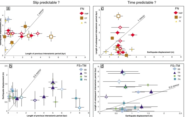
[70] Figure 4 examines whether the earthquake slips and times data might be related by simple “slip-predictable” or “time-predictable” functions [e.g., Schwartz and Coppersmith, 1994, and references therein]. We have discriminated the north-ern and southnorth-ern faults that slip at different rates, 1–2 mm/yr and 0.2–0.5 mm/yr, respectively (Table 3 and discussion below). If the size (i.e., slip) of an earthquake on a fault is governed by the length of the interseismic time before that earthquake, the slip-time data would fall on the dashed line in Figures 4a and 4b that represents the
average slip rate of the fault. Clearly, neither relation char-acterizes the analyzed faults. Conversely, if the timing of an earthquake on a fault is governed by the amount of slip released by the prior earthquake, the slip-time data would fall on the dashed line in Figures 4c and 4d that represents the average slip rate of the fault. Clearly, this relation is not valid either for any of the analyzed faults. Therefore, our data offer no support to the classical slip- and time-predictable earthquake models.
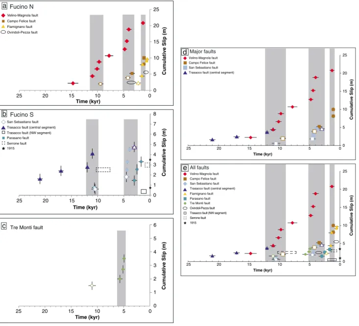
[71] Figure 5 examines the cumulative earthquake slip versus time on the different faults and systems. The well-constrained trench data have been included (Table 1). 5.2.1. FN Fault System
[72] Nine, five, and five events were recognized from the 36Cl analysis on the VMF, CF, and FI faults, respectively
(Figure 5a). Two events were also identified in trenches on the Ovindoli-Pezza fault (referred to as OP in following). Over the time of ~ 10 ka when the VMF and the CF faults have a common record, about twice more earthquakes occurred on VMF and produced a cumulative slip almost twice as large (~ 17 m on VMF versus ~ 10 m on CF). These cumulative slips would convert into mean slip rates of ~ 2 mm/yr on the VMF, and half that on the CF. The record on FI and OP is too short to derive a meaningful slip rate. On the four faults, the coseismic slips have a similar range, of 1.0–3.5 m (Tables 1 and 4). On the VMF and CF master faults, the slip record shows a similar pattern, with short, ~ 1–2 ka long periods of multiple, clustered earthquakes (grey vertical bands in Figure 5a), interrupted by 1–4 ka long more quiescent phases with no or one event.
The periods of more intense activity are roughly the same for the two faults, around ~ 1–1.5 ka, ~ 3–5 ka, and ~ 9–11 ka. The secondary OP fault also likely broke during the two most recent phases of clustered earthquakes. The FI fault broke in two large events during the most recent phase of intense activity, but also broke in three events when the two master faults were quiescent.
[73] The 1915 Avezzano earthquake revealed a case where several nearby parallel faults broke in concert during the same event. We might thus wonder whether the events that we found as having a fairly similar age on distinct yet nearby faults could be the same events. As all coseismic slips found per event are larger than 1 m (but for one event on FI) and more generally on the order of 2 m (Table 3; see also Table 1 for trench data), it is unlikely that two (or more) sim-ilar-age events found on two distinct, ~ parallel faults be the same earthquake since summing a minimum of two events would produce a 3–4 m slip, a value too high to be realistic (see section 5.4 for a discussion on the slips). In contrast, in the cases where two (or more) similar-age events are found on distinct, yet collinear faults, it is possible that the two (or more) events are the same earthquake, as their slips would not add. The two events recognized in trenches on the OP fault might thus be the similar-age events identified with
36Cl on the collinear CF fault.
5.2.2. FS Fault System
[74] Five, five, and four events were recognized with36Cl on the SB, TR (central segment), and PA faults, respectively (Figure 5b). Four events are also suggested from trench data
1 mm/yr a c 0 1 2 3 4 5 6 0 1 2 3 4 5 6 7 8 9
Length of subsequent interseismic period (kyr) Earthquake displacement (m)
Slip predictable ? Time predictable ?
1 mm/yr VMF CF FI 0 1 2 3 4 0 1 2 3 4 5 6 7 8 9 Earthquake displacement (m)
Length of previous interseismic period (kyr)
VMF CF FI b d 0 1 2 3 4 5 6 7 8 9 0 0,5 1 1,5 2 2,5
Length of subsequent interseismic period (kyr)
Earthquake displacement (m) 0.5 mm/yr 0.5 mm/yr SB PA TR TM 0 0,5 1 1,5 2 2,5 0 1 2 3 4 5 6 7 8 9 Earthquake displacement (m)
Length of previous interseismic period (kyr)
SB PA TR TM FS+TM FS+TM FN FN
Figure 4. Examining the slip- and time-predictable hypotheses. Symbols are larger for major faults. Full symbols indicate well-constrained data, while empty symbols indicate less well-constrained data. Most events recorded on (a) FN faults or (b) FS faults are not slip predictable nor time predictable (c and d) since most points do not fall on the dashed line that corresponds to the mean slip-rate of the faults (1 mm/yr and 0.5 mm/yr for FN and FS faults, respectively). Note that, since the Tre Monti fault has a low slip rate, it is shown with the FS faults.