HAL Id: hal-01681557
https://hal.archives-ouvertes.fr/hal-01681557
Submitted on 14 May 2018
HAL is a multi-disciplinary open access archive for the deposit and dissemination of sci-entific research documents, whether they are pub-lished or not. The documents may come from teaching and research institutions in France or abroad, or from public or private research centers.
L’archive ouverte pluridisciplinaire HAL, est destinée au dépôt et à la diffusion de documents scientifiques de niveau recherche, publiés ou non, émanant des établissements d’enseignement et de recherche français ou étrangers, des laboratoires publics ou privés.
Recent climate hiatus revealed dual control by
temperature and drought on the stem growth of
Mediterranean Quercus ilex
Morine Lempereur, Jean-Marc Limousin, Frédéric Guibal, Jean-Marc
Ourcival, Serge Rambal, Julien Ruffault, Florent Mouillot
To cite this version:
Morine Lempereur, Jean-Marc Limousin, Frédéric Guibal, Jean-Marc Ourcival, Serge Rambal, et al.. Recent climate hiatus revealed dual control by temperature and drought on the stem growth of Mediterranean Quercus ilex. Global Change Biology, Wiley, 2017, 23 (1), pp.42-55. �10.1111/gcb.13495�. �hal-01681557�
RECENT CLIMATE HIATUS REVEALED DUAL CONTROL BY TEMPERATURE AND
1
DROUGHT ON THE STEM GROWTH OF MEDITERRANEAN
Q
UERCUS ILEX2 3 4
Running head: STEM GROWTH AND CLIMATE HIATUS
5 6
Morine Lempereur1, 2*, Jean-Marc Limousin1, Frédéric Guibal3, Jean-Marc Ourcival1, Serge 7
Rambal1, 4, Julien Ruffault1, 5, 6, and Florent Mouillot7 8
9
1 Centre d'Ecologie Fonctionnelle et Evolutive CEFE, UMR 5175, CNRS - Université de Montpellier -
10
Université Paul-Valéry Montpellier – EPHE, 1919 Route de Mende, 34293 Montpellier Cedex 5, France
11
2 Agence de l’Environnement et de la Maîtrise de l’Energie, 20, avenue du Grésillé- BP 90406, 49004
12
Angers Cedex 01, France
13
3 Institut Méditerranéen de Biodiversité et d’Ecologie marine et continentale (IMBE), UMR 7263
14
CNRS, Marseille Université – IRD – Avignon Université, Europôle de l'Arbois, BP 8013545,
Aix-15
en-Provence Cedex 4, France
16
4 Universidade Federal de Lavras, Departamento de Biologia, CP 3037, CEP 37200-000, Lavras, MG,
17
Brazil
18
5 Irstea, UR REVOVER, 3275 route Cézanne, CS 40061, 13182 Aix-en-Provence cedex 5, France
19
6 CEREGE UMR 7330, CNRS – Aix-Marseille Université, Europôle de l’Arbois, BP 8013545,
Aix-en-20
Provence Cedex 4, France
21
7 Centre d'Ecologie Fonctionnelle et Evolutive CEFE, UMR 5175, CNRS - Université de Montpellier -
22
Université Paul-Valéry Montpellier – EPHE - IRD, 1919 Route de Mende, 34293 Montpellier Cedex 5,
23
France
24 25
*Author for correspondence: Morine Lempereur 26 Tel: +33(0)467613292 27 Email: morine.lempereur@cefe.cnrs.fr 28 29
Keywords: Basal area increment, climate change, climate-growth response, climate hiatus, 30
drought, growth duration, growth phenology, Quercus ilex 31
32
Type of Paper: Primary Research Article 33
2
Abstract
35
A better understanding of stem growth phenology and its climate drivers would improve 36
projections of the impact of climate change on forest productivity. Under a Mediterranean 37
climate, tree growth is primarily limited by soil water availability during summer, but cold 38
temperatures in winter also prevent tree growth in evergreen forests. In the widespread 39
Mediterranean evergreen tree species Quercus ilex, the duration of stem growth has been shown 40
to predict annual stem increment, and to be limited by winter temperatures on the one hand, and 41
by the summer drought onset on the other. We tested how these climatic controls of Q. ilex 42
growth varied with recent climate change by correlating a 40-year tree ring record and a 30-43
year annual diameter inventory against winter temperature, spring precipitation, and simulated 44
growth duration. Our results showed that growth duration was the best predictor of annual tree 45
growth. We predicted that recent climate changes have resulted in earlier growth onset (-10 46
days) due to winter warming and earlier growth cessation (-26 days) due to earlier drought 47
onset. These climatic trends partly offset one another, as we observed no significant trend of 48
change in tree growth between 1968 and 2008. A moving-window correlation analysis revealed 49
that in the past, Q. ilex growth was only correlated with water availability, but that since the 50
2000s, growth suddenly became correlated with winter temperature in addition to spring 51
drought. This change in the climate-growth correlations matches the start of the recent 52
atmospheric warming pause also known as the ‘climate hiatus’. The duration of growth of Q. 53
ilex is thus shortened because winter warming has stopped compensating for increasing drought
54
in the last decade. Decoupled trends in precipitation and temperature, a neglected aspect of 55
climate change, might reduce forest productivity through phenological constraints and have 56
more consequences than climate warming alone. 57
58
L
IST OF ABBREVIATIONS USE IN PAPER 59FS: Long-term field survey of diameter at breast height (DBH), measured from 1986 to 2013. 60
RW: Ring-width series, measured from 1942 to 2008. 61
AD: Automatic dendrometer series, measured from 2004 to 2013. 62
Puéchabon station: weather station located in the study site since 1984. 63
SML station: weather station located in St Martin-de-Londres, 12 km away from the study site, 64
data available from 1966 to 2013 (Meteo France). 65
TJFM: Mean of daily temperature from January to March (°C). 66
PAMJ: Sum of precipitation from April to June (mm). 67
WSI: Water stress integral, a time-cumulated drought severity index (MPa day) 68
t0: Day of year when stem growth starts 69
3 t1: Day of year when stem growth stops in early summer
70
∆tt0-t1: Duration of the period between t0 and t1 computed for each set of simulated phenological
71
thresholds. 72
BAI: Basal area increment of the stems, expressed in mm² year-1
73
PET: Potential evapotranspiration (mm) 74
4
I
NTRODUCTION76
Stem growth, recorded in annual tree rings, is a synthetic surrogate of carbon input in 77
standing biomass (Babst et al., 2014) and an index for tree vitality and fitness (Bigler & 78
Bugmann 2003; Benito-Garzon et al., 2013). In return, it is the record of the yearly climatic 79
conditions that have enabled stem growth over a period lasting from decades to centuries (Fritts 80
1976; Briffa et al., 2002). Understanding the factors that control stem growth is therefore crucial 81
to assess the impact of past and future climate change on forests, but remains a major scientific 82
issue due to a series of currently unresolved uncertainties. 83
First, the climate sensitivity of tree growth is generally considered to depend on 84
photosynthesis and respiration fluxes because most process-based models assume that tree 85
growth is carbon limited (Davi et al,. 2006; Gaucherel et al., 2008; Keenan et al., 2011). Carbon 86
allocation to sapwood is therefore the key process driving the carbon sink, and is at the heart of 87
tree growth simulations in most terrestrial biosphere models (e.g. Sitch et al., 2003; 88
Friedlingstein et al., 2006; Fisher et al., 2010). Several allocation schemes exist (e.g. fixed 89
allocation, the pipe model, and hierarchical allocation between plant organs, Schippers et al., 90
2015), but there is accumulating experimental evidence that cambial activity (sink limitation) 91
is more sensitive to environmental stressors than carbon assimilation (source limitation; Körner 92
2003; Fatichi et al., 2014; Guillemot et al., 2015; Körner 2015; Delpierre et al., 2016a). Taking 93
sink limitation into account in terrestrial biosphere models is thus likely to improve their ability 94
to simulate past and future forest productivity (Leuzinger et al., 2013; Fatichi et al., 2014), but 95
a better characterization of the phenology and climate sensitivity of wood formation is a 96
prerequisite (Rossi et al., 2011; Rossi et al., 2014; Lempereur et al., 2015; Delpierre et al., 97
2016a; Delpierre et al., 2016b). 98
Second, global climate change may simultaneously exert opposing influences on forest 99
functioning, and these impacts are difficult to disentangle. For example, increased water use 100
efficiency due to atmospheric CO2 enrichment is sometime reported to increase tree growth in
101
spite of concurrently increasing aridity (Martinez-Vilalta et al., 2008; Koutouvas 2013), but the 102
opposite finding is far more common (Peñuelas et al., 2011). Warming also exerts opposing 103
impacts on tree growth: on one hand it increases the length of the growing season (Keeling et 104
al., 1996; Dragoni et al., 2011) while on the other hand it exacerbates atmospheric evaporative
105
demand and hence water limitation (Angert et al., 2005; Zhao & Running, 2010). Warming 106
may therefore affect tree growth positively (e.g. Rossi et al., 2014) or negatively (e.g. Brzostek 107
et al., 2014) depending on the ecosystem under consideration.
5 Third, relationships between tree growth and climate may change under the influence of 109
climate change (e.g. Briffa et al., 1998; Büntgen et al., 2006; Carrer & Urbinati 2006; D’Arrigo 110
et al., 2008). A classic example of this phenomenon is the so-called ‘divergence problem’ in
111
northern forests, which is a weakening of the positive temperature response of tree growth in 112
strongly temperature limited ecosystems since the middle of the 20th century (D’Arrigo et al., 113
2008). The consequence of such temporal variations in tree growth sensitivity to climate is that 114
empirical dendrochronological models based on statistical links between tree growth and 115
climate cannot be extrapolated to long term historical and future climate conditions with 116
confidence (e.g. Gea-Izquierdo et al., 2013; Subedi & Sharma 2013). 117
Fourth, climate change itself is a complex phenomenon that may result in changes in the 118
mean climate (IPCC 2014), in the frequency of extreme climatic events (Meehl & Tebaldi 2004) 119
and in seasonality (Giorgi et al., 2011; Ruffault et al., 2013), all of which may have contrasted 120
impacts on tree growth and function. In addition, climate change is not monotonous and the 121
recent slowing down of the warming trend, early identified by Easterling & Wehner (2009) and 122
later called the 'climate hiatus' (Trenberth & Fasullo, 2013), is currently a topic of increasing 123
scientific interest. But if most scientific studies have focused on explaining the causes and 124
processes behind this ‘climate hiatus’ or pause in atmospheric warming (Meehl et al., 2011; 125
Balmaseda et al., 2013; England et al., 2014; Steinman et al., 2015), few have attempted to 126
assess its ecological consequences, especially for processes that are highly sensitive to climate, 127
such as tree growth. 128
In water limited ecosystems, where forest productivity is primarily limited by drought 129
(Churkina & Running 1998; Zhao & Running 2010), the supply of water from rainfall appears 130
to be the key variable to explain tree growth (Babst et al., 2013). In the case of the 131
Mediterranean species Quercus ilex, the conclusions of dendrochronological studies converge 132
more specifically to identify winter and spring rainfall amounts as the key drivers of annual 133
stem growth (Gutiérrez et al., 2011). In contrast, Q. ilex stem growth is generally poorly 134
correlated with winter and spring temperatures. Daily measurements of basal area increment 135
over an eight year period (2004-2011) with automatic dendrometers in a Q. ilex forest, 136
demonstrated that the duration of spring growth was an accurate predictor of annual stem 137
growth (Lempereur et al., 2015). After observing that the duration of spring growth was 138
determined by winter temperature for growth start and a lower threshold of predawn plant water 139
potential of -1.1 MPa for growth cessation, Lempereur et al. (2015) proposed a new hypothesis 140
wherein the annual growth of Q. ilex is under the dual control of winter temperature and spring 141
water limitation. 142
6 In this contextual framework, we used both tree ring records over a 40-year period and 143
an annual diameter inventory over a 30-year period to (i) test whether the stem growth 144
phenology approach proposed by Lempereur et al. (2015) can explain Q. ilex growth over a 145
long retrospective period with different growth estimation methods, (ii) assess the relative 146
importance of drought and temperature in limiting Q. ilex growth under a Mediterranean 147
climate, and (iii) evaluate the stationarity of these limitations in recent decades. In particular, 148
we aimed to identify whether any temporal shift in the climate controls of Q. ilex growth 149
(drought or temperature plus drought) are concomitant to, and the functional consequence of, 150
the recent pause in atmospheric warming. 151
152
M
ATERIALS ANDM
ETHODS 153Site description
154
The study site is located 35 km north-west of Montpellier (southern France), on a flat 155
plateau, in the Puéchabon state forest (43°44’29”N, 3°35’45”E, 270 m a.s.l.). This forest has 156
been managed as a coppice for centuries and the last clearcut took place in 1942. Vegetation is 157
largely dominated by a dense overstory of the evergreen oak Quercus ilex. In 2014, the average 158
top canopy height was 5.5 m and the stem density was 4700 (±700) stems ha-1. Understory
159
evergreen species, Buxus sempervirens, Phyllirea latifolia, Pistacia lentiscus and Juniperus 160
oxycedrus, compose a sparse shrubby layer (height < 2 m) with less than 25% cover. The
161
climate is Mediterranean, with 80% of the rainfall occurring between September and April. 162
Average annual precipitation for the 1984-2013 period was 916 mm (550 to 1549 mm). Mean 163
annual temperature over the same period was 13.2 °C with a minimum in January (5.5 °C) and 164
a maximum in July (22.9 °C). The very shallow bedrock has a hard Jurassic limestone origin. 165
The volumetric fraction of stones and rocks averages 0.75 in the top 0-50 cm and 0.90 below. 166
The stone free fine fraction of the soil in the 0-50 cm layer is a homogeneous silty clay loam 167
(USDA texture triangle) comprising 38.8% clay, 35.2% silt and 26% sand. 168
169
Monitoring annual stem growth
170
Stem diameter at breast height (DBH) was measured annually from 1986 to 2013 on 319 171
trees distributed in eight circular plots (diameter 20 m) within an area of 2 ha. The 319 trees 172
used in this field survey (hereafter FS, Fig. 1) were selected so as to include all the diameter 173
7 size classes in 1986. DBH was measured every winter under dry conditions using a diameter 174
tape at a height identified by a paint mark on the stem. In January 2008, the stem diameters 175
were distributed as follows: 58% < 8 cm DBH, 24% between 8 and 10 cm and 18% >10 cm. 176
Because the smaller size classes exhibited a very low growth and a high mortality rate, we 177
restricted our analysis to the 125 trees with a DBH > 8 cm in 2008 to obtain a stronger growth 178
signal (Table 1). From 2004 to 2013, stem growth was measured more frequently and with 179
greater accuracy using automatic band dendrometers on a subset of trees in two neighboring 180
plots (for more details, see Lempereur et al., 2015). Automatic dendrometers (ELPA-98, 181
University of Oulu, Finland; hereafter AD) were set up at a height of 1.3 m above the ground 182
on 6 to 12 trees with DBH > 7 cm. The two datasets (FS and AD) were strongly correlated 183
during their overlapping period (Table 1), thus demonstrating the relative accuracy of FS in 184
estimating the annual growth of the largest trees. 185
186
187
Fig. 1 Chronological timeline of the main data sources used in this study. Stem growth series: automatic
188
dendrometers (AD), field survey (FS) of stem diameter at breast height (DBH) and ring width series (RW).
189
Climatic data: Puéchabon meteorological station and St Martin-de-Londres (SML) meteorological station.
190 191
Dendrochronological procedures
192
In 2005 and 2008, 15 and 12 stems, respectively, were selected among the largest size 193
classes of the field survey (FS) sample (10 cm < DBH < 16 cm) and cut down to measure ring-194
width chronology. Cross sections were collected at stump height, air dried, sanded and polished 195
(40 to 400 grit). The longest growth radii in each cross section were selected and compared 196
pairwise under a binocular magnifier. In old coppiced oaks, rings are narrow and sometimes 197
not clearly visible after 40 years of cambial age; consequently only 12 of the sampled stems 198
could be cross dated with confidence, seven stems in 2005 and five stems in 2008. The first 199
ring was formed in 1942 after the clearcut in winter 1941-1942, so data in the ring width series 200 T im e (y e a r ) 1 9 6 0 1 9 8 0 2 0 0 0 R W F S A D S M L 19 68 19 86 20 08 20 13 P u e c h a b o n M e te o S ta ti o n S te m G ro w th 20 04
8 (hereafter RW) were obtained from 1942 to 2008 (Table 1, Fig. 1). Cross dating was facilitated 201
by the presence of frost rings corresponding to the severe winters of 1963, 1985 and 1987. 202
These rings, typical for years with severe freezing episodes, were abnormally wide because the 203
cells of their initial area were crushed and dislocated, a typical constraint on tree ring 204
interpretation in woody species under a Mediterranean climate (Cherubini et al., 2003). This 205
particular feature made them useful as markers for cross dating but prevented the reliable 206
measurement of annual stem growth, so these years were excluded from subsequent analyses. 207
Cross correlation coefficients on annual tree ring indices calculated among the 12 individual 208
series were all higher than 0.6 (P-value<0.05). The ring width measured at stump height and 209
along the longest growth radius was then rescaled to the tree DBH at the time of the cut. This 210
required correction for the tapering between stump height (20 cm) and breast height (130 cm) 211
as well as correction for the bark thickness (see Fig. S1 for details). The average tree ring width 212
after rescaling, which was used to calculate the basal area increment (BAI), was 954 µm 213
(CV = 48%) between 1942 and 2008, and 792 µm (CV = 38%) over the period 1968-2008 used 214
in our study. 215
216
Table 1 Main characteristics of the three growth series used in the study, automatic dendrometer (AD), field survey
217
(FS) and ring width (RW), over their respective complete temporal series and their overlap periods. Coefficients
218
of correlation (r) between FS and AD over the period 2004-2013 and between RW and FS over the period
1987-219
2008 are given (P-value < 0.05: *; P-value < 0.001: ***).
220
Characteristics of the growth series
Method Period Mean BAI (mm²) DBH 2008 (cm) Sample size
AD Auto Dendro 2004-2013 185.8(±70,00) 11.1 (±2.45) 12
FS Diameter tape 1987-2013 154.4 (±44,47) 10.5 (±1.85) 125
RW Ring width 1968-2008 204.6 (±55,39) 12.7 (±1.75) 12
Correlations on overlap periods
Ovelap period Growth series Mean BAI (mm²) r
AD vs. FS 2004-2013 AD 185.8(±70.00) 0.90 (***) FS 142.3 (±55.37) FS vs. RW 1987-2008 FS 158.2 (±44.68) 0.55 (*) RW 196.2(±45.00) 221 Climate variables 222
The Puéchabon meteorological station (hereafter Puéchabon) is located in a clearing 223
200 m away from the study plot and has provided daily on-site climate data since 1984 (Fig. 1). 224
Precipitation was measured with a tipping bucket rain gauge (ARG100; Environmental 225
Measurements, Sunderland, UK) calibrated to 0.2 mm per tip and placed 1 m above the ground, 226
air temperature was recorded with a MP100 sensor (Rotronic, Bassersdorf, Switzerland) at a 227
9 height of 2 m, and net radiation was measured with a pyranometer (SKS1110; Skye Instruments, 228
UK) at a height of 2 m above the ground. 229
To extend our analysis before 1984, we used climate variables (daily rainfall, daily 230
minimum and maximum temperature) from the St Martin-de-Londres meteorological station 231
(hereafter SML; 43°47’06’’N; 3°43’48’’E, altitude 194 m a.s.l., located about 12 km away from 232
the study site; source Meteo-France) over the period 1966-2013 (Fig. 1). The mean daily 233
temperature was calculated as the average of the minimum and maximum daily temperature. 234
The climate data from SML station were compared to on-site measurements in the overlap 235
period 1984-2013 (Table S1 and Fig. S2). The comparison showed close agreement for 236
temperature but a higher rainfall amount in SML than in Puéchabon. No significant biases 237
(slope not different from 1, and distance to origin not different from 0) were observed between 238
the two meteorological stations in the two crucial variables related to stem growth: the mean 239
temperature from January to March (TJFM) and the sum of precipitation from April to June
240
(PAMJ; Fig. S2).
241
Daily solar radiation at the SML station was calculated from the processing chain 242
described in Kumar et al. (1997). In the first step, theoretical clear sky solar radiation (Ra) was
243
calculated from the daily timing of sunrise and sunset, the bi-hourly sun azimuthal angle and 244
the atmospheric transmittance according to longitude using R Cran Packages ‘RAtmosphere’ 245
and ’oce’. No topographical effects were taken into consideration. Actual solar radiation (Rs, in
246
MJ m-2 day-1) was then calculated from maximum and minimum daily temperature (T
max and
247
Tmin, respectively) and the clear sky theoretical radiation following the Hargreaves equation:
248
, where the adjustment coefficient kRs was set to 0.16 for interior
249
location (Allen et al., 1998). Results of the Hargreaves equation were validated against solar 250
radiation measured in Puéchabon since 1998. 251
252
Modeling predawn leaf water potential and water stress integral
253
Soil water storage integrated over the rooting depth, c.a. 4.5 m, was measured during the 254
vegetative periods of 1984-1986 and from July 1998 to August 2009 at approximately monthly 255
intervals, using a neutron moisture gauge (503DR Hydroprobe, CPN, Concord, CA, USA). 256
Discrete measurements were interpolated at a daily time step using the soil water balance model 257
described by Rambal (1993) and further used by Rambal et al. (2014). The model was driven 258
by daily values of incoming solar radiation, minimum and maximum temperatures, and rainfall 259
amount. Potential evapotranspiration was computed using the Priestley-Taylor equation 260
aRs
s k T T R
10 (Priestley & Taylor, 1972). The reduced major axis (RMA) regression between neutron 261
moisture gauge measurements and model simulations yielded an R2 of 0.93, the slope was
262
0.94 ± 0.05 (P < 0.0001, n = 91) and the intercept not significantly different from 0. Soil water 263
storage and soil water potential were linked by a Campbell-type retention curve (Campbell, 264
1985) whose parameters are strongly dependent on soil texture (Saxton et al., 1986; Rambal et 265
al., 2003). Predawn leaf water potential used for model validation was measured about eight
266
times a year between April and October from 2003 to 2009 on a subsample of four trees among 267
those equipped with automatic dendrometers (see Limousin et al., 2012). RMA regressions 268
between measured and simulated values of predawn leaf water potential yielded an R2 of 0.84, 269
the slope was 0.93 ± 0.05 (P < 0.0001, n = 54), and the intercept was not significantly different 270
from 0. We used the simulations of predawn water potential rather than soil water content, as 271
the former is more closely linked with plant functioning (Rambal et al., 2003). The daily 272
simulations of predawn water potential were performed with the climate data from the 273
Puéchabon and SML stations for the periods 1984-2012 and 1966-2012, respectively. The water 274
stress integral (WSI), defined by Myers (1988) as the seasonally or yearly sum of predawn 275
water potential, was used as a drought severity index to quantify annual or seasonal water stress. 276
277
Duration of spring basal area increment: calculations of dates t0 and t1
278
The dates of stem growth phenology that bounded the spring growth period, the DOY 279
(day of the year) when stem growth starts (hereafter t0) and the DOY when stem growth stops
280
in early summer (hereafter t1, Fig. S3), were estimated for each year. The relationships between
281
t0 or t1 and climate variables were calibrated by Lempereur et al. (2015) on observations of t0
282
and t1 obtained with automatic dendrometers from 2004 to 2011. Briefly, t0 was defined as the
283
first day at which basal area exceeded the culmination of the previous year, and t1 as the first
284
day when BAI became null or negative (see Lempereur et al., 2015 for methodological details). 285
t0 and t1 were estimated using climate data from both Puéchabon and the nearby SML station
286
over their corresponding timeframes. t0 was predicted by a nonlinear relationship with the mean
287
temperature from January to March (TJFM). The relationships were fitted between t0 and TJFM
288
measured in Puéchabon (t0 = 849.2*exp(-0.6436 TJFM)+121; R² = 0.95; RMSE = 2.6 days;
289
Lempereur et al., 2015) and between t0 and TJFM measured in SML (t0 = 4300*exp(-0.943
290
TJFM)+124.4; R² = 0.95; RMSE = 2.3 days; Fig. S4). t1 was predicted by the DOY when the
291
plant water potential simulated using climate data from Puéchabon reached a threshold of -292
1.1 MPa (R² = 0.75; RMSE = 7 days, Lempereur et al., 2015), corresponding to a DOY when 293
11 the plant water potential simulated using climate data from SML reached a threshold of -294
1.1 MPa + ɛ (with ɛ = -0.1; R² = 0.73; RMSE = 13.5 days) due to the slight differences in 295
temperature and precipitation between the two stations (see Fig. S5). The duration ∆tt0-t1
296
corresponds to the duration of the period between t0 and t1 and was computed for each pair of
297
simulated phenological thresholds. 298
299
Data processing and statistical analyses
300
Annual stem growth (DBH and ring widths) was converted into annual basal area 301
increments (BAI, expressed in mm² year-1) for the two data series. Analyses were performed 302
with averaged BAI values of 125 and 5-12 individual trees for FS and RW, respectively. The 303
year 1992 presented two periods when predawn plant water potential fell below the threshold 304
of -1.1 MPa, in spring and autumn (Fig. S6). This unusual bi-modal drought prevented us from 305
determining the duration ∆tt0t1 so 1992 was excluded from subsequent analyses. The growth
306
series BAIFS included measurements that appeared to be outliers compared to BAIRW or BAIAD
307
for the years 2002 and 2010 (see Fig. S7). In 2002, BAIFS was particularly low when BAIRW
308
was close to the expected value, and in 2010, BAIFS was clearly higher than the BAIAD value.
309
Because BAIFS is less accurate than the other two methods, and was calculated as the difference
310
between two subsequent measurements of DBH, these two values were considered to be 311
unreliable and excluded from the analyses performed on BAIFS.
312
To investigate the links between tree growth and climate, we computed the correlations 313
between our two different growth datasets (FS and RW) and a set of relevant climate predictors. 314
For each correlation tested, we reported the Pearson’s correlation coefficient and its 315
significance based on the standard bootstrap method with 1000 samples taken from the original 316
distribution of climate and tree ring data. Within each sample, the number of observations was 317
random and followed a geometric distribution. We used the ‘treeclim’ R package built upon the 318
DENDROCLIM2002 statistical tool dedicated to tree ring analysis (Biondi & Waikul, 2004; 319
Zang & Biondi, 2015). Climate predictors were derived from temperature and precipitation at 320
monthly, seasonal and annual time scales, and from our functional index of spring growth 321
duration (∆tt0t1). To test for the stationarity of the drought and temperature controls over the
322
studied period, we also performed the same bootstrap sampling Pearson correlation analysis on 323
a 10-year moving window along the whole series. 324
The temporal trends in stem growth and climate variables were characterized using both 325
trend tests and breakpoint analyses. Temporal trends in time series were estimated using the 326
12 Theil-Sen test (Sen 1968) from the ‘openair’ R cran package, applied on a 1000 block bootstrap 327
simulations to account for auto-correlated variables (Kunsch 1989), with the block length set to 328
n/3, n being the length of the time series. Temporal breakpoints in the time series were assessed 329
by computing the yearly F-statistic (sequential F-test) and the supF statistic was then used to 330
test for their significance. 331
332
RESULTS
333Sensitivity of stem growth to the dual temperature-drought drivers
334
335
Fig. 2 Time series of annual stem basal area increment (BAI) for the ring width series (RW; 1942-2008), the
long-336
term field survey (FS; 1986-2013) and the automatic dendrometer series (AD; 2004-2013). Error bars are standard
337
errors among the sampled trees (see Table 1 for sample size).
338 339
Annual stem growth (BAIRW) from 1942 to 2008 exhibited two distinct phases, with a
340
significant breakpoint around 1967 (Fstat = 81.96; P-value<0.0001; Fig. 2). The first phase 341
(1942-1967) lasted 25 years after the clearcut and showed a linear increase of 5.5 (±0.62) mm² 342
y-1 in annual BAI. This phase, which corresponds approximately to the cut frequency formerly
343
used in the traditional management of this Q. ilex coppice (Floret et al., 1992), was 344
characterized by incomplete canopy cover and notable self-thinning. The second phase (1968-345
2008) showed a stabilization of BAIRW around a mean value of 203.8 (±54.84) mm² y-1. The
346
influence of climate on stem growth was consequently only considered from 1968 on, to avoid 347
the confounding effects caused by changes in competition, space-filling and self-thinning 348
during the first phase. 349
The two long-term growth series BAIRW and BAIFS were significantly correlated with each
350
other during their overlap period 1986-2008 (r = 0.55, P-value < 0.05, Table 1). Both series of 351
BAI exhibited large between year variations (coefficient of variation, CV = 27% and 29% for 352 T im e ( y e a r ) B A I (m m ² y -1 ) 1 9 6 0 1 9 8 0 2 0 0 0 0 1 0 0 2 0 0 3 0 0 4 0 0 A D F S R W
13 BAIRW and BAIFS, respectively). The minimum value of BAI was recorded in 2006 for both
353
series: BAIRW = 114 mm² y-1 (SE = 36.5 mm² y-1) and BAIFS = 58 mm² y-1 (SE = 13.2 mm² y
-354
1). The maximum BAI was recorded in 1977 for RW (BAI
RW = 348 mm² y-1, SE = 22.1 mm² y
-355
1) and in 2001 for FS (BAI
FS = 246 mm² y-1; SE = 20.8 mm² y-1, vs. BAIRW = 213 mm² y-1; 356 SE = 24 mm² y-1.2). 357 358 359
Fig. 3 Relationship between yearly basal area increment (BAI) and the duration of the spring growth period (∆t t0-360
t1). Ring width (RW, dark grey circle) is shown for the period 1984-2008 and field survey (FS, light grey square) 361
for the period 1986-2013. The linear relationships between ∆tt0-t1 and BAIRW (dark grey line; BAIRW = 1.34*∆t t0-362
t1 + 122.9; R² = 0.56; P-value < 0.001) or BAIFS (light grey line; BAIFS = 1.09*∆tt0-t1 + 95.5; R² = 0.35; P-363
value < 0.01) are represented. Error bars are standard errors.
364 365
The DOY of the start (t0) and stop (t1) of the spring stem growth, simulated over the period
366
1984-2013 using climate data from the Puéchabon station, occurred on average in mid-May 367
(DOY 133, SD = 9.9 days) and early July (DOY 184, SD = 23.5 days), respectively. The growth 368
duration ∆tt0-t1 varied considerably among years (CV = 50%) with values ranging from 2 days
369
in 1995 to 95 days in 2008 (Fig. 3). BAI was linearly correlated with ∆tt0-t1 for both stem growth
370
series (R² = 0.56; P-value < 0.0001 and R² = 0.35; P-value < 0.01 for RW and FS respectively; 371
Fig. 3). Moreover, ∆tt0-t1 was the best explanatory variable for the inter-annual variations in
372
BAIRW compared to other climate variables over the period 1984-2008 (Table 2; 3). We thus
373
concluded that the dual control of annual stem growth by temperature and precipitation, stated 374
by Lempereur et al. (2015) for the period 2004-2011, remained valid for a longer retrospective 375
period and when growth is measured with less accuracy than with automatic dendrometers. The 376
intercepts of the linear relationships between BAI and ∆tt0-t1, which represent the residual
377
autumnal growth (Lempereur et al., 2015), differed significantly between the two BAI series 378
(F = 17.97; P-value < 0.001), with 122.9 (±34.42) mm² y-1 and 95.5 (±39.09) mm² y-1 for RW 379
and FS, respectively (Fig. 3). By contrast, the slopes of these relationships did not differ 380 tt 0 - t 1(d a y ) B A I (m m ² y -1 ) 0 2 0 4 0 6 0 8 0 1 0 0 0 1 0 0 2 0 0 3 0 0 F S R W
14 significantly between RW and FS (F = 0.46; P-value > 0.05), and the common slope equals 381
1.23 mm² day-1. The sensitivity of BAI
RW to ∆tt0-t1 was thus identical to the sensitivity of BAIFS.
382
Furthermore, neither the extension of the study period to 1968-2008 nor the switch in 383
meteorological stations from Puéchabon to SML, removed the significant correlation between 384
BAIRW and ∆tt0-t1 (R² = 0.31; P-value < 0.001; Table 2).
385 386
Table 2 Mean Pearson’s correlation coefficients (and significance derived from a 1000 classical bootstrap
387
sampling) between chronologies of annual stem growth (BAI) and the main phenology explanatory variables. The
388
correlations are given using climate variables measured in Puéchabon field surveys (FS) over the period
1986-389
2013 and ring width (RW) over the period 1984-2008, and climate data from the SML meteorological station over
390
the period 1968-2008 for RW (see Fig. 1). The explanatory variables tested were the start and stop growth dates
391
(t0 and t1, respectively) and the duration of stem growth (∆tt0-t1). The coefficient of correlation (r) and the level of 392
statistical significance (*P-value < 0.05; **P-value < 0.01; ***P-value < 0.001) are given. Significant correlations
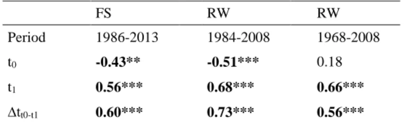
393 are in bold. 394 FS RW RW Period 1986-2013 1984-2008 1968-2008 t0 -0.43** -0.51*** 0.18 t1 0.56*** 0.68*** 0.66*** ∆tt0-t1 0.60*** 0.73*** 0.56*** 395
Stem growth response to climate trends from 1968 to 2013
396
Over the longer period 1968-2008, ∆tt0-t1 was not a better predictor of BAI than the sum
397
of spring precipitation (PAMJ) or t1 alone (r = 0.75; P-value < 0.001 and r = 0.66; P-value < 0.001
398
respectively; Table 2, 3), and we also observed a loss of correlation between BAI and t0
399
(r = 0.18; P-value = 0.31; Table 2). 400
PAMJ was the main explanatory climate variable for t1 (over the period 1968-2008:
401
r = 0.80; P-value<0.001) and it exhibited no temporal trend between 1968 and 2013 (P-402
value = 0.31; Fig. 4b). However, spring water limitation increased (WSI in spring: -403
0.48 MPa day y-1; P-value<0.001; Fig. 4d, Table S3) as a result of increasing spring potential
404
evapotranspiration (PET; +0.028 mm day-1 y-1; P-value<0.001; Fig. 4c, Table S3). This trend 405
in PET was mainly due to the significant warming trend in spring temperatures throughout the 406
period 1968-2013 (+0.07°C y-1; P-value<0.001; Fig. 4a, Table S3). As a result, drought onset 407
t1 exhibited a temporal trend toward earlier dates (-0.57 day y-1; P-value<0.01; Fig. 5). The
408
correlation between BAIRW and PAMJ remained significant, however, throughout most of the
409
1968-2008 period (Fig. 6a). 410
15
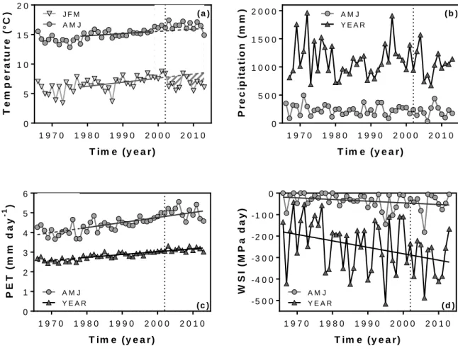
Fig. 4 Temporal trends in (a) spring (AMJ) temperature (grey circles) and winter (JFM) temperature (light grey
412
inverted triangles), (b) mean annual precipitation (dark grey triangles) and AMJ precipitation (grey circles), (c)
413
mean annual potential evapotranspiration (ETP; dark grey triangles) and AMJ ETP (grey circles) and (d) annual
414
water stress integral (WSI, dark grey triangles) and AMJ three months WSI (grey circles). The solid lines represent
415
significant temporal trends (P-value<0.05). The dashed lines represent the extended trend for temperature after
416
1998, or before 1978 for PET. The effect of the warming pause on the JFM temperature (panel a) is shown by the
417
hatched area between the points and the regression line, the vertical dotted lines indicate the start of the winter
418
warming pause in 2002.
419 420
In parallel, TJFM increased significantly throughout the period (+0.04 °C y-1;
P-421
value<0.05; Fig. 4a) which led to a significant trend of t0 toward earlier dates (-0.21 day y-1;
P-422
value<0.05; Fig. 5). However, a pause in the atmospheric winter warming occurred in the last 423
decade. This warming pause is apparent in the discrepancy between actual and expected TJFM
424
obtained from the temporal trend built over the period 1978-1998. The year 1978 was chosen 425
because it corresponds to the onset of a rapid warming phase in the Northern Hemisphere (Mann 426
et al., 1999). Similarly, the year 1998 was considered as the onset of the climate hiatus
427
observations (IPCC 2014). We used the period 1978-1998 to build the reference trend line and 428
extrapolate expected TJFM values over the 1999-2013 period. We then tested for a breakpoint in
429
the anomalies between observed and expected TJFM over the whole period. Such a breakpoint
430
was identified in 2002, indicating a significant slowing down in winter warming after this date 431 T im e (y e a r ) T e m p e r a tu r e ( ° C ) 1 9 7 0 1 9 8 0 1 9 9 0 2 0 0 0 2 0 1 0 0 5 1 0 1 5 2 0 J F M A M J ( a ) T im e (y e a r ) P r e c ip it a ti o n ( m m ) 1 9 7 0 1 9 8 0 1 9 9 0 2 0 0 0 2 0 1 0 0 5 0 0 1 0 0 0 1 5 0 0 2 0 0 0 A M J Y E A R ( b ) T im e (y e a r ) P E T ( m m d a y -1 ) 1 9 7 0 1 9 8 0 1 9 9 0 2 0 0 0 2 0 1 0 0 1 2 3 4 5 6 A M J Y E A R ( c ) T im e (y e a r ) W S I (M P a d a y ) 1 9 7 0 1 9 8 0 1 9 9 0 2 0 0 0 2 0 1 0 - 5 0 0 - 4 0 0 - 3 0 0 - 2 0 0 - 1 0 0 0 A M J Y E A R ( d )
16 (Fstat = 21.52; P<0.001; Fig. 4a). This temporal pattern was also observed at seven other 432
meteorological stations in the region surrounding our study site (Table S4 and Fig. S8), thus 433
confirming the regional occurrence of the globally observed climate hiatus (Trenberth & 434
Fasullo, 2013). The date of growth onset (t0) was very sensitive to the warming pause in TJFM
435
and a breakpoint in the t0 trend was observed in 2002 (Fstat = 21.52; P<0.001; Fig. 5). We also
436
observed that the start of the winter warming pause coincided with a change in the climate 437
controls on annual stem growth. Indeed, the correlation between BAI and TJFM, which was only
438
significant over one 10-year window between 1968 and 1994, became constantly significant 439
from the time window 1995-2004 on (Fig. 6b). 440
441
Table 3 Mean Pearson’s correlation coefficients and significance (derived from a 1000 classical bootstrap
442
sampling) between annual stem growth (BAI) or spring growth duration (Δtt0t1) and monthly or seasonal 443
precipitation (P, in mm) and temperature (T, in °C) for RW data series. The climate data from Puéchabon and
444
Saint Martin-de-Londres meteorological stations were used for the periods 1984-2013 and 1966-2013,
445
respectively. The coefficients of correlation (r) and the level of statistical significance (*P-value < 0.05;
**P-446
value < 0.01; ***P-value < 0.001) are given. Significant correlations are in bold.
447 BAI Δtt0t1 1984-2008 1968-2008 1984-2013 1966-2013 T P T P T P T P November (t-1) 0.06 -0.08 -0.23* -0.03 0.07 0.24 -0.31* -0.03 December (t-1) 0.30** 0.08 -0.07 -0.04 0.25 0.04 -0.06 -0.03 January 0.50*** -0.06 0.02 0.15 0.51*** 0.03 0.34*** 0.14 February 0.37* -0.27* -0.02 0.06 0.20 -0.16 0.22 0.02 March 0.34** -0.17 -0.10 0.21 0.41*** -0.10 0.11 0.19* April 0.05 0.23 0.00 0.33* -0.11 0.48*** -0.07 0.24* May 0.12 0.47*** -0.23 0.57*** 0.08 0.37 -0.25* 0.48** June -0.46** 0.21 -0.65*** 0.44*** -0.01 0.00 -0.24* 0.22 July -0.56*** 0.32** -0.54*** 0.36** -0.26 -0.13 -0.42*** 0.01 August -0.08 -0.04 -0.30** 0.07 0.03 0.24* -0.37*** 0.08 September -0.39* -0.39* -0.42*** -0.25* -0.18 -0.35 -0.34*** -0.10 October -0.13 -0.13 -0.14 -0.04 -0.18 -0.34** -0.22 -0.15 Jan. Feb. March 0.48*** -0.20 -0.05 0.18 0.47* -0.11 0.32** 0.15 Apr. May June -0.15 0.53*** -0.38*** 0.75*** -0.02 0.49* -0.23 0.55***
June Aug. Sept. -0.42** -0.34 -0.51* -0.14 -0.18 -0.30 -0.45*** -0.05
from Nov(t-1) to Oct 0.04 -0.11 -0.37* 0.25* 0.15 0.01 -0.21* 0.17
448
The temporal trends in t0 and t1, both toward earlier dates (-10 and -26 days,
449
respectively) offset each other to some extent until 2002 and resulted in a non-significant trend 450
in ∆tt0-t1. After 2002, the prolonged trend in t1 continued to decrease while t0 stabilized, thereby
451
leading to a sudden shortening of the growing season (Fig. 5). The timing of this phenological 452
reduction was concomitant with the appearance of a significant relationship between TJFM and
17 BAI (Fig. 6b). The decline in ∆tt0-t1 induced by the winter warming pause resulted in a decrease
454
in BAIRW after 2002. This decreasing trend over time become significant after the 10-year time
455
window 1997-2006 (Fig. 7a,b). BAIFS exhibited a similar decreasing trend in the same period,
456
but of lower amplitude and not significant. 457
458
459
Fig. 5 Onset of phenological stem growth (t0, pale grey inverted triangles) and end of stem growth (t1, grey circles) 460
from 1966 to 2013, expressed as day of the year (DOY).The effect of the warming pause on t0 is shown by the 461
hatched area between the points and the regression line over the 1978-1998 period.
462 463
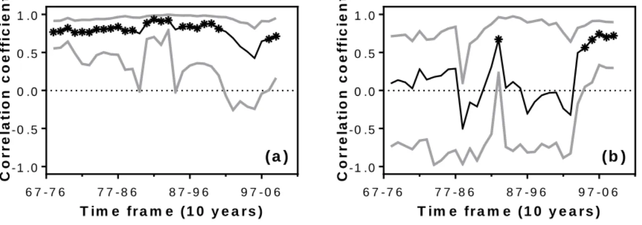
464 465
Fig. 6 Temporal variations in the bootstrapped Pearson’s correlation coefficients between (a) BAIRW and PAMJ, 466
and (b) BAIRW and TJFM over 10-year moving windows. The black curve represents the correlation coefficient and 467
the grey curves the upper and lower confidence intervals at a significance level α = 0.05. Asterisks identify the
468
time windows with significant correlations.
469 470 T im e (y e a r ) t0 & t1 ( D O Y ) 1 9 7 0 1 9 8 0 1 9 9 0 2 0 0 0 2 0 1 0 1 0 0 1 5 0 2 0 0 2 5 0 t0 t1 T im e fr a m e ( 1 0 y e a r s ) C o r r e la ti o n c o e ff ic ie n t - 1 .0 - 0 .5 0 .0 0 .5 1 .0 7 7 - 8 6 8 7 - 9 6 9 7 - 0 6 ( a ) 6 7 - 7 6 T im e fr a m e ( 1 0 y e a r s ) C o r r e la ti o n c o e ff ic ie n t - 1 .0 - 0 .5 0 .0 0 .5 1 .0 7 7 - 8 6 8 7 - 9 6 9 7 - 0 6 (b ) 6 7 - 7 6
18
Fig. 7 Temporal trend over 10-year moving windows of (a) mean annual stem growth from 1968 to 2008 and from
471
1987 to 2013 for ring width (RW, dark grey circles) and field surveys (FS, grey squares), respectively. Error bars
472
are standard errors. (b) Slopes of the linear trends of BAI for the two series. The asterisks indicate time windows
473
with a significant trend (p<0.05). The dotted vertical lines in both panels indicate the first time window with a
474
significant relationship between BAIRW and TJFM after the warming pause. 475
476
DISCUSSION
477Growth duration as a predictor of annual stem growth
478
The duration of spring stem growth (∆tt0-t1) was the best explanatory variable of yearly
479
basal area increment for both BAIFS and BAIRW after 1984. This confirms earlier results
480
obtained with automatic dendrometers over a shorter period and a smaller sample of trees 481
(Lempereur et al., 2015), and therefore validates ∆tt0-t1 as a robust estimator of Q. ilex annual
482
stem growth over long time scales and large samples. The two independent samplings we used 483
here differed markedly in the number of trees measured, the measurement method and its 484
precision. FS corresponds to a large number of trees (125 trees) representing a broader tree size 485
distribution but measured with a less precise resolution (0.3 mm of DBH), while RW was 486
measured on a small sample of large dominant trees (12 trees) but with a better resolution 487 T im e fr a m e ( 1 0 y e a r s ) B A I (m m ² y -1 ) 1 0 0 1 5 0 2 0 0 2 5 0 7 7 - 8 6 8 7 - 9 6 9 7 - 0 6 ( a ) R W F S 6 7 - 7 6 0 7 - 1 6 T im e fr a m e ( 1 0 y e a r s ) li n e a r t r e n d o f B A I (m m 2 y -2 ) - 1 5 - 1 0 - 5 0 5 1 0 1 5 7 7 - 8 6 8 7 - 9 6 9 7 - 0 6 (b ) R W F S 6 7 - 7 6 0 7 - 1 6
19 (0.01 mm of radius). Average stem growth was lower for BAIFS than for BAIRW, but both
488
responded linearly and with the same sensitivity to ∆tt0-t1 (Fig. 3).
489
The spring stem growth duration ∆tt0-t1 is defined as the length of the period between the
490
onset of spring stem growth (t0) and the date of growth cessation caused by summer drought
491
(t1). Lempereur et al. (2015) observed that t0 was well predicted by winter temperature, and that
492
t1 occurred when the leaf predawn water potential dropped below a threshold of -1.1 MPa. A
493
similar approach was used by Rossi et al. (2011, 2014) who linked the stem growth of boreal 494
black spruce with the duration of xylem growth delimited by cold temperatures in spring and 495
autumn, and by Delpierre et al. (2016a) who linked the growth of temperate oak to the timing 496
of the summer growth cessation controlled by water limitation. By identifying the climatic 497
limits for cell division and elongation, the temporal delimitation of tree growth duration is an 498
innovative way of improving simulation of forest carbon sink response to climate change 499
(Fatichi et al., 2014). Tree growth has generally been simulated using two types of models: 500
statistical dendroclimatological models, which are empirical and may lead to marked 501
uncertainties when extrapolated to future climate scenarios (e.g. Gea-Izquierdo et al., 2013; 502
Babst et al., 2014); and process based models that link tree growth to carbon assimilation (e.g. 503
Sitch et al., 2003; Friedlingstein et al., 2006; Gaucherel et al., 2008; Keenan et al., 2011), 504
ignoring experimental evidence showing a direct, and generally more limiting, climate control 505
of plant growth (Körner, 2003; Muller et al., 2011). Projecting tree growth based on growth 506
phenology as in Rossi et al. (2011) and Lempereur et al. (2015) merges the biological realism 507
of the first approach, i.e. a direct link between climate and growth, with the mechanistic 508
understanding of tree physiology used in process based models, and be a significant step 509
forward in projecting the response of forest ecosystems to climate change (Delpierre et al., 510
2016b). Showing that growth duration is an adequate predictor of tree growth for long time 511
series datasets (40 years in our study) and coarse temporal resolution (annual diameter 512
measurements) is thus an important preliminary. 513
Nevertheless, the spring growth duration approach remains limited by both its conditions of 514
applicability and the large proportion of the growth variability not explained by ∆tt0-t1. The
515
particular case of the year 1992, with its bi-modal drought in spring and autumn and its well-516
watered summer (Fig. S6), suggests that ∆tt0-t1 can only be used as a descriptor of stem growth
517
phenology in years with typical Mediterranean seasonality and a drought period occurring in 518
summer. While the lowest threshold of predawn water potential below which stem growth is 519
prevented certainly remains valid for any drought seasonality (Hsiao & Xu, 2000; Muller et al., 520
2011; Lempereur et al., 2015), we hypothesize that the relationship between stem growth and 521
20 the duration of periods with adequate growth conditions (the rate of growth) varies in years 522
with peculiar phenology. Variations in the rate of growth may also account for the unexplained 523
variability in the BAI against ∆tt0-t1 relationships (44% and 65% for RW and FS, respectively;
524
Fig. 3). Finally, the relative extent of autumn growth compared to spring growth would deserve 525
more detailed investigation. Lempereur et al. (2015) observed that autumn growth explained 526
only approximately 30% of annual stem growth and was strongly determined by spring 527
conditions, but its magnitude over long time periods and under climate change conditions 528
remains to be described. 529
530
Dual limitation of growth by winter cold and spring-summer drought
531
Summers in the Mediterranean region are typically characterized by the concomitance of 532
low rainfall, high temperature and high solar radiation, while winters are cold and humid. 533
Consequently, vegetation functioning is limited by water deficit in summer and by low 534
temperatures in winter (Mitrakos, 1980; Terradas & Savé, 1992). A cessation of growth during 535
cold and dry periods is frequently observed in Mediterranean trees which display a bi-phasic 536
growth pattern over the year (Cherubini et al., 2002; Campelo et al., 2007; Montserrat-Marti et 537
al., 2009; Camarero et al., 2009, Gutiérrez et al., 2011).
538
The sensitivity of growth to water deficit is well established in the literature (Lockhart 539
1965; Hsiao & Xu, 2000; Muller et al., 2011), as is the negative impact of drought on ring width 540
(Fritts, 1976). Previous dendroclimatological studies generally stated that spring to early-541
summer precipitation was the main driver of annual stem growth of Q. ilex (Gutiérrez et al., 542
2011). More precisely, it is the start of the dry season, defined by a threshold of soil water 543
deficit that was identified as the main determinant of variations in inter-annual growth (Maselli 544
et al., 2014; Lempereur et al., 2015). The predominant effect of the timing of drought induced
545
growth cessation on annual stem growth is not limited to Mediterranean ecosystems, as a similar 546
effect has been observed in mesic temperate forests (Brzostek et al., 2014; Delpierre et al., 547
2016a). In our study, we defined the start of the dry season as a critical threshold of predawn 548
plant water potential of -1.1 MPa. This threshold is biologically meaningful because water 549
potential affects the cell turgor pressure necessary for cell growth (Hsiao & Xu, 2000), and it 550
has the other advantage of comprehensively accounting for climate and local soil conditions in 551
a single metric (Ruffault et al., 2013). It is, however, a more complex index to calculate than 552
climatic indices of drought as it requires substantial knowledge of soil and vegetation 553
characteristics, and accurate meteorological data at the daily time scale. Consequently, the 554
21 uncertainty on t1 was higher than the uncertainty on t0, especially when meteorological data
555
from SML (located at a distance of 12 km from the study site) was used instead of on-site data, 556
but t1 nonetheless remained a good predictor of annual stem growth for whichever period (Table
557 2). 558
Depending on the species and on the local bio-climate, a minimum temperature 559
threshold ranging from +4 °C to +7 °C is required for stem growth to occur (Körner, 2003; 560
Rossi et al., 2007; Deslauriers et al., 2008; Gruber et al., 2010; Swidrak et al., 2011; Lempereur 561
et al., 2015). The onset of stem growth can be assessed from winter temperature (Delpierre et
562
al., 2016b), thus the mean winter temperature directly impacts the duration of cambium activity
563
and wood formation (Rossi et al., 2011). However, there is no consensus in 564
dendrochronological studies of the Mediterranean Q. ilex that winter temperature is a good 565
predictor of annual BAI, and both negative (Zhang & Romane 1990; Paton et al., 2009; Gea-566
Izquierdo et al., 2009) and positive correlations (Campelo et al., 2009; Nijland et al., 2011; 567
Gea-Izquierdo et al., 2011) between annual stem growth and winter temperature have been 568
reported. In our study, a positive correlation between growth and winter temperature was 569
observed over the period 1984-2008 (r = 0.48, P<0.001; Table 3), in accordance with 570
Lempereur et al. (2015), but the relationship was not significant for the period 1968-2008, either 571
with t0 or with TJFM.
572
Taken together, these results suggest that summer drought is the main limiting factor for 573
Q. ilex growth, which is to be expected under the dry Mediterranean climate. Nevertheless, the
574
contrasted growth responses to winter temperature depending on the study concerned, or on the 575
period of interest, led us to investigate the impact of recent climate change on Q. ilex growth in 576
more detail. 577
578
Can warmer winter temperature compensate for earlier summer drought under climate
579
change?
580
From 1968 to 2008, the annual and spring amounts of precipitation were stable (Fig. 4b), 581
but water limitation increased (Fig. 4d) due to increasing potential evapotranspiration with 582
rising temperature in spring and summer (Fig. 4a and c), in accordance with regional 583
observations (Ruffault et al., 2013). Consequently, we simulated an earlier occurrence of 584
drought onset (t1, -26 days on average) along with an earlier growth onset, although to a lesser
585
extent (t0, -10 days; Fig. 5), which, taken together resulted in a non-significant decrease in
586
growth duration. The positive effect of warming on ecosystem functioning and tree growth 587
22 through a longer growing season has been widely observed in temperature limited boreal and 588
temperate forests (Keeling et al., 1996; Menzel et al., 2006; D’Arrigo et al., 2008; Dragoni et 589
al., 2011). However, in water limited regions, like the Mediterranean, warming is generally
590
considered to be an aggravating factor for drought, mainly because of increased evaporative 591
demand (Angert et al., 2005; Zhao & Running, 2010; Park et al., 2012). Consequently, climate 592
warming in the Mediterranean usually reduces tree growth (Jump et al., 2006; Sarris et al., 593
2007; Peñuelas et al., 2008; Piovesan et al., 2008; Martin-Benito et al., 2010). Our results thus 594
mitigate this widely accepted conclusion and illustrate the peculiar parallel controls driven by 595
temperature, such that the benefit of an earlier stem growth is cancelled out by earlier drought 596
onset mostly caused by increasing evaporative demand. 597
The effect of temperature on t1, mediated by PET, may also explain why the correlation
598
with growth was better for t1 than for PAMJ over the period 1984-2008, when temperatures
599
increased significantly, but not over the longer period 1968-2008. Actually, spring PET, like 600
temperature, did not increase significantly until the early 1980s (Fig. 4a, c), suggesting that, in 601
the past, inter-annual variability in precipitation may have been a stronger driver of drought 602
onset. Alternatively, the lack of on-site precipitation measurements before 1984 may mean that 603
t1 estimates based on SML are less closely linked to on-site conditions than three-month
604
cumulated precipitation. The correlation in precipitation amounts between Puéchabon and SML 605
actually increases with longer temporal resolutions. 606
Winter warming may also have a positive impact on stem growth by delaying growth 607
cessation in autumn, thereby partly compensating for earlier drought onset. However, the 608
phenology of autumn growth cessation appears to be less variable than that of t0 (Lempereur et
609
al., 2015), possibly because it is concurrently driven by photoperiod. Moreover, warm winters
610
may even impact Q. ilex growth negatively if the species requires winter chilling, as is the case 611
of the deciduous Quercus species (Fu et al., 2015). 612
613
A Mediterranean “divergence problem”
614
When looking at the temporal variations in the correlations between stem growth and 615
climate variables, we observed an abrupt and significant increase in the sensitivity of stem 616
growth to temperature in the early 2000s, while at the same time, its response to precipitation 617
weakened (Fig. 6a, b). Temporal changes in the response of tree growth to climate have been 618
observed in a wide range of climates and tree species in recent decades (e.g. Briffa et al., 1998; 619
Büntgen et al., 2006; Carrer & Urbinati 2006; Jump et al., 2007; D’Arrigo et al., 2008). The 620
23 ‘divergence problem’ in northern forests has been defined as the tendency for tree growth at 621
previously temperature limited sites to undergo a weakening of their temperature response 622
concurrent with an increasing sensitivity to drought (D’Arrigo et al., 2008). Our results suggest 623
a Mediterranean ‘divergence problem’ according to which tree growth in water limited 624
Mediterranean ecosystems undergo a weakening of their response to spring-summer 625
precipitation and an increasing sensitivity to winter temperatures. Similar reports of temporal 626
changes from water driven to increasingly temperature driven tree growth in water limited 627
ecosystems have already been reported for beech forests in northeast Spain (Jump et al., 2007), 628
black pine forests in Spain (Martin-Benito et al., 2010), and Scots pine, European larch and 629
black pine in Switzerland (Feichtinger et al., 2014). These observations differ from ours by 630
reporting an increase of the overall negative effect of warming on tree growth. Nevertheless, 631
they collectively point to the increasing influence of temperature on the growth of previously 632
water limited trees. 633
634
Concurrent increase in drought and warming: a keystone aspect of climate change revealed
635
during the recent warming hiatus
636
A keystone result of our study is the sudden significance of the growth-temperature 637
relationship occurring from the 1995-2004 time window on (Fig. 6b). In parallel, we observed 638
lower winter temperatures than would have been expected on the basis of continuous climate 639
warming (Fig. 4a). This regional pattern is therefore comparable to the globally observed 640
“warming hiatus” (Easterling & Wehner 2009; Trenberth & Fasullo 2013). Our results suggest 641
that these recent cooler winter temperatures resulted in later growth onset and led to an 642
increased temperature constraint on the duration of stem growth. In the meantime, the constraint 643
exerted by the water deficit increased constantly from 1968 onward with neither breakpoints 644
nor changes in the trend line (Fig. 4d, 5). As a result, the stem growth of Q. ilex was significantly 645
correlated only with water deficit in the past, but the shorter growth period after the 2000s 646
revealed the dual control by winter temperatures and spring-summer water deficit. The pause 647
in climate warming in turn disrupted the precarious balance between increasing winter 648
temperatures and increasing spring-summer water deficit, which temporarily sustained stem 649
growth until the end of the 1990s (Fig. 7). This is, to our knowledge, the first example of a 650
‘divergence problem’ in the tree growth-climate relationship triggered not by a continuous 651
climate change but instead by the warming pause. This recent warming pause, a still 652
controversial aspect of climate change (Lewandowsky et al., 2015; Wehner & Easterling 2015), 653
24 is mainly caused by the variations in Atlantic and Pacific multidecadal oscillations (Steinman 654
et al., 2015), and produced globally heterogeneous patterns of breakpoint in the recent warming
655
trend (Ying et al., 2015), with an enhanced effect on winter temperature in Eurasia (Li et al., 656
2015). It is however, likely to be reversed in the coming decades (Steinman et al., 2015). 657
Whether a future re-acceleration of climate warming in the Mediterranean would compensate 658
for increasing water deficit by phenological stimulation of earlier tree growth again, or on the 659
contrary, further exacerbate drought stress remains an open and important question. Studying 660
trends in targeted and concurrent climate variables such as temperature and drought should fully 661
capture the complexity of climate change impacts (Mazdiyani & Aghakouchak 2015). Climate 662
projections for the Mediterranean region forecast an increase in potential evapotranspiration 663
and a decrease in summer precipitation by the end of the 21th century (Gao & Giorgi 2008; 664
Ruffault et al., 2014), which are likely to move the onset of drought forward more strongly than 665
the onset of spring growth (Lempereur et al., 2015). Together with the current growth limiting 666
winter temperatures, these future trends in drought features could lead to a sharp reduction in 667
forest productivity and an increase in tree mortality in Mediterranean Q. ilex forests. 668
669
ACKNOWLEDGEMENTS
670M. Lempereur benefited from a doctoral research grant provided by the French Environment
671
and Energy Management Agency (ADEME). Long term meteorological data were provided by
672
Météo France. The Puéchabon experimental site belongs to the SOERE F-ORE-T, which is
673
supported annually by Ecofor, Allenvi and the French national research infrastructure
ANAEE-674
F. The authors would like to thank Alain Rocheteau, Karim Piquemal and David Degueldre for
675
their technical assistance, and the two anonymous reviewers for their detailed and helpful
676
reviews of the manuscript.
677
REFERENCES
678Allen RG, Pereira LS, Raes D, Smith M (1998) Crop evapotranspiration-Guidelines for 679
computing crop water requirements-FAO Irrigation and drainage paper 56. FAO, Rome, 680
300. 681
Angert A, Biraud S, Bonfils C, Henning CC, Buermann W, Pinzon J, Tucker CJ, Fung I (2005) 682
Drier summers cancel out the CO2 uptake enhancement induced by warmer springs.
683
Proceedings of the National Academy of Sciences of the United States of America, 102, 684
10823-10827. 685