HAL Id: halshs-00556992
https://halshs.archives-ouvertes.fr/halshs-00556992
Preprint submitted on 18 Jan 2011HAL is a multi-disciplinary open access archive for the deposit and dissemination of sci-entific research documents, whether they are pub-lished or not. The documents may come from teaching and research institutions in France or abroad, or from public or private research centers.
L’archive ouverte pluridisciplinaire HAL, est destinée au dépôt et à la diffusion de documents scientifiques de niveau recherche, publiés ou non, émanant des établissements d’enseignement et de recherche français ou étrangers, des laboratoires publics ou privés.
Céline Carrere
To cite this version:
Céline Carrere. Regional Agreements and Welfare in the South: When Scale Economies in Transport Matter. 2011. �halshs-00556992�
Document de travail de la série Etudes et Documents E 2007.26 R REEGGIIOONNAALLAAGGRREEEEMMEENNTTSSAANNDDWWEELLFFAARREEIINNTTHHEESSOOUUTTHH:: W WHHEENNSSCCAALLEEEECCOONNOOMMIIEESSIINNTTRRAANNSSPPOORRTTMMAATTTTEERR Céline Carrère*1 37 p.
1 The paper has been greatly improved by the comments and suggestions of Jaime de Melo. I would
also like to thank Olivier Cadot, Stéphane Calipel, Riccardo Faini, Patrick Guillaumont, Thierry Mayer, and Alexandre Skiba for helpful discussions. The usual disclaimer applies.
Abstract
This paper focuses on two issues that challenge the accepted pessimistic view that regional trade agreements (RTAs) between developing countries in welfare terms by taking into account scale economies in transport. First, how is the standard welfare analysis of an RTA affected by the endogeneity of transport costs (i.e. by the joint determination of trade quantities and transport costs)? Second, what are the long-run consequences of endogenous transport costs for welfare if worldwide free trade is achieved through RTAs? A standard model of inter and intra-industry trade is augmented by a “hub-and-spoke” transport network structure, where the standard “iceberg” transport cost model is contrasted with one in which transport costs depend on the distance between trade partners, the volume of trade, and the level of development. Under a plausible parameterization for scale economies in transport, regional liberalization will have persistent effect on trade flows through an irreversible effect on regional transport costs that improves welfare. Free trade achieved under an RTA leads to permanently higher welfare than under
multilateral liberalization.
JEL Classification: F12, F15, R4, O1, D6.
Keywords: Regional Integration, Welfare, Transport Costs, Economies of Scale, Developing countries.
* Corresponding Author:
Address: Department of Econometrics and Political Economy, School of Business Administration (HEC), Lausanne University, Internef, CH-1015 Lausanne, Switzerland. Phone : 00 41 21 692 34 72 / Fax : 00 41 21 692 33 65 /Email : Celine.Carrere@unil.ch
1. Introduction
Ever since Viner’s (1950) pioneering study, the ambiguous impact on welfare of Regional Trade Agreements (RTAs) has been analyzed in terms of the relative magnitude of trade creation and trade diversion. Recently, transport costs have been recognized among the factors that could influence this trade-off. Wonnacott and Lutz (1989) first argued that RTAs are more likely to be welfare enhancing when formed among what they called “natural trading partners”, i.e. countries geographically closed. Krugman (1991a, 1991b) developed and popularized this idea in a monopolistically competitive framework, showing that continental free trade areas (i) decrease welfare unambiguously with zero inter-continental transport costs, (ii) increase welfare unambiguously with prohibitive inter-continental transport costs. Relying on simulations where transport costs take continuous values between zero and prohibitive values, Frankel, Stein and Wei (1996), conclude that all else constant, a preferential trade agreement is more likely to be welfare enhancing (i) the more remote the continental trading partners are from the rest of the world (i.e. the larger inter-continental transport costs are) thereby limiting potential trade diversion and (ii) the more “natural” (i.e. the closer in distance) trading partners are thereby fostering potential trade creation (see Baier and Bergstrand (2004) for a complete survey on simulation results).
The “natural trading partner” argument potentially concerns 77% of existing RTAs. It is particularly relevant for RTAs between developing countries (or regional “South-South” agreements), notably in Sub-Saharan Africa (SSA) where many RTAs are implemented between neighboring countries that are quite remote from major world markets.2 Actually, though developing countries benefit from some recent technological advances that reduce transport costs, extensive
documentation attests to their still facing considerably higher transport costs than developed countries. Shipping costs, for instance, are dramatically higher for
2 Of the 208 PTAs notified to the GATT/WTO in 2004, 160 are implemented between countries of
a same region. Source: World Trade Organization secretariat and Author’s calculation. To name a few: MERCOSUR, the customs union involving Argentina, Brazil, Paraguay and Uruguay; the Association of Southeast Asian Nations (ASEAN), the South Asian Preferential Trade Agreement (SAPTA), the Southern African Custom Union (SACU), The Economic and Monetary Union of West Africa (UEMOA), the Economic and Monetary Community of Central Africa (CEMAC), Common Market for Eastern and Southern Africa (COMESA), the Southern African Development Community (SADC).
developing countries according to the price quotes from international freight forwarders (see Hummels, 1999, Limao and Venables, 2001 or Busse, 2003). Geographic impediments (such as landlockness), poor transport infrastructure (Limao and Venables, 2001) contribute to explain these high transport costs in developing countries. Moreover, as shown by Hummels (2001), Clark, Dollar and Micco (2002) and Djankov et al. (2006), other cost-raising factors like time in shipping or custom clearance further increase transport costs for developing countries. Anderson and Van Wincoop (2004) conclude that trade costs represent a significant handicap for developing countries.
So far, the literature has characterized the environment describing developing countries by assuming “iceberg” transport costs (à la Samuelson, 1954) which supposes that only a constant fraction of the quantity shipped actually arrives (as if “only a fraction of the ice exported reaches its destination as un-melted ice”). Virtually, all simulation models so far analyzing the welfare of regional trade liberalization have relied on this representation of transport costs, thus ignoring the potential effect of scale economies in transport (e.g. Frankel, Stein and Wei, 1996, Nitsch, 1996, Frankel, 1997, Spilimbergo and Stein, 1998, Baier and Bergstrand, 2004). Simply put, transport costs are assumed unaffected by equilibrium quantities traded.
There is now strong direct evidence of the importance of scale economies in shipping costs. Using a dataset covering the bilateral trade of six importers (Argentina, Brazil, Chile, Paraguay, Uruguay, and the United States) with all exporters worldwide in 1994, Hummels and Skiba (2004) find that doubling trade quantities along a route reduces shipping costs by 12 percent for all countries on that route. The same order of magnitude is reported by Tomoya and Nishikimi (2002) : a 1% increase in the number of ships on a particular route between Japan and each of the Southeast Asian ports resulted in a 0.12% reduction in the freight rates. Fink, Mattoo and Neagu (2002), studying the liner transport price on all US imports carried by liners from 59 countries in 1998, also conclude to significant economies of scale with regard to traffic originating from the same port.
What are the sources of these scale economies in shipping? Hummels and Skiba (2004) identify three main sources of reductions in transport costs as trade quantities increase. First, a densely traded route allows for effective use of
“hub-and-spoke” shipping economies.3 Second, increased quantities traded encourage the introduction of specialized transport technologies along a route (as
standardized containerized shipping for maritime transport). A third source of scale benefits lies in pro-competitive effect on pricing (limiting the monopoly markups of for instance the “liner conferences”) to which we return shortly.
In the model developed in this paper, I focus on the second source of scale economies in transport: the adoption of new transport technology when trade increases (the first source is exogenously imposed by a pre-determined “hub-and-spoke” transport network built into the model)4. As to the endogenous market structure, I take the extreme, but arguably realistic case for small developing countries, of a transport sector provided by a monopolist. Hence, in the model, according to the volume traded, a monopoly shipper decides whether to pay sunk costs (such as investment in infrastructure) in order to adopt a lower marginal cost transport technology.
The justification for this approach stems from the importance of the welfare-reducing effects of high transport costs associated with low trade volume ,and further exacerbated by low competition intensity. For example the problem of “cargo reservation schemes” and liner conferences whereby only one shipping company will cover a route because of low traffic densities leads to monopoly practices (see the evidence in Hummels 1999, Fink, Mattoo and Neagu, 2002). Furthermore, in this environment, the adoption of new technologies such as containerization may be delayed by such market structure (see Hummels, 1999).
Moreover, the set-up developed in this paper takes into account a critique that has been raised against the “natural trading partner hypothesis”, namely that
differences in costs determined by comparative advantage could be an important factor weighing against the benefits of trade between close partners. As noted by Panagariya (1998, p.294), “distant partners can be efficient suppliers of certain products due to other cost advantages despite the fact that they must incur higher transport costs.” In a comment to a model by Frankel, Stein and Wei (1996),
3 For instance, as explained by Hummels and Skiba (2004), small container vessels move
quantities into a hub where containers are aggregated into much larger and faster containership for longer hauls.
Krugman (1998, p.115) also notes that the restriction of identical economic size may not be innocuous and “surely makes a major difference when we try to model the effects of integration”. In this paper, I take the view that differences in costs related to economic size, is sufficient to capture the concerns raised by Panagariya (1998) since larger countries will have lower production costs, while at the same time maintaining the parsimony afforded by an otherwise symmetric modeling framework.
Based on this evidence and stylized description of the transport sector in
developing countries, the paper addresses the issue of the welfare costs of RTAs by answering two questions. First, how is the standard welfare analysis of regional trade liberalization affected by the endogeneity of transport costs (i.e. if trade quantities and transport costs are jointly determined)? By boosting bilateral trade among members, regional liberalization exploits scale economies along regional routes (through the adoption of new transport technologies) and then leads to a reduction in transport costs.
Second, what are the consequences of endogenous transport costs for welfare if worldwide free trade is achieved via preferential trade agreements rather than via multilateral trade liberalization?5 Suppose that the long-run objective is worldwide free trade. With exogenous transport costs (i.e. transport costs independent to the level of trade), the welfare achieved under worldwide free trade is independent of the chosen path (i.e. via regionalism or multilateral liberalization). Now, suppose endogenous transport technology. Sequencing then matters because of sunk costs in transportation. South-South RTAs will then generate persistent effects on member countries’ trade flows and welfare when they liberalize trade by regional route.
The paper is organized as follows. Section 2 adapts a standard monopolistic competition model with inter-industry trade in an agricultural product produced under constant returns to scale and a manufacturing sector under monopolistic
5This question is inspired from Freund (2000)’s paper which addresses the sequencing issue raised
by Bhagwati (1993). Using a model with imperfect competition, she shows that a sequencing in which liberalization takes place via an RTA leads to a greater expansion in world output than immediate free trade because of sunk costs to expand trade and investment first realized within the regional borders. Actually, permanent effects from RTAs arise if firms undertake irreversible investments that reduce production and distribution network costs before free trade is achieved.
competition with scale economies in production borrowed from Spilimbergo and Stein (1998). An explicit “hub-and-spoke” transport sector with a profit
maximizing monopolist choosing endogenously his transport technology completes this stylized representation of production and trade in a developing country. Section 3 applies the model to a 4-continent world with two types of countries: North and South which differ by size and economies of scale. As a start, section 3 compares the welfare evolution according to the degree of tariff
preference within symmetric regional bloc (i.e. blocs within neighbor countries of South-South and North-North type) with exogenous / endogenous transport costs. Section 4 then tackles the sequencing issue by contrasting welfare results when worldwide free trade is achieved through a regional path vs. a multilateral non-discriminatory path. Section 5 studies how sensitive the results are to the “hub-and-spoke” transport network assumption. Results are also extended for North-South agreements. Section 6 concludes.
2. Overview of the Model6
2.1. Basic Setup
The model includes 3 sectors augmented by a transport sector developed in section 2.2. Following Spilimbergo and Stein (1998), we assume 3 sectors: agriculture, intermediate inputs, and manufactures, and 2 factors of production: capital (K) and labor (L). We consider 2 types of countries, which differ only in their capital endowment. In “poor” countries (subscript, p), each individual is endowed with 1 unit of capital, as well as 1 unit of labor. In “rich” countries (subscript r), each individual owns 1 unit of labor and k units of capital (where k>1).Imposing symmetry within groups and a similar model structure across country groupings improves significantly the tractability of the model while capturing in a stylized way, the main features necessary to include transport costs and preferential trade policy.
A representative consumer in country i share a Cobb-Douglas utility function given by:
6
(
) (
)
1{
}
0 1 ;
i mi ai i
U = C α C −α <α ≤ = r p (1)
With Cm a i( ) the consumption of manufactures (agriculture) in country i, α (1−α) the share of consumer’s income spent on manufactures (agriculture).
Technology is Ricardian throughout. In Agriculture, a homogeneous good is produced under constant returns to scale with labor as the only input with labor productivity set at unity by choice of units. Production is then given by:
{
}
, ;
ai ai i
q =L = r p (2)
Therefore, under perfect competition:
pai =wi, i=
{
r p;}
(3) with paithe price of agriculture and withe wage in country i.7A Final manufactured good is produced for domestic consumption under a Dixit-Stiglitz technology for intermediate inputs with constant returns to scale, each intermediate input entering symmetrically into its production:
(
)
{
}
1 , 0 1 , 1.. ; mi ji i q =∑
cθ θ <θ < m j = n i = r p (4) jic being the consumption of the jth variety produced in country i and θ capturing the extent of product differentiation across intermediates of different origin (“love of variety”) . As θ approaches 1,
σ
=1/(1−θ
)→ ∞, and intermediates of different origin become perfect substitutes, intra-industry trade is eliminated and only inter-industry trade remains.Intermediate inputs are also produced with a Ricardian technology with capital as input under monopolistic competition. Increasing returns to scale is captured by assuming a fixed cost, γ , and a constant marginal cost, β :
ji ji K =γ+βx ⇔ ji , 1..
{
;}
ji i K x γ j n i r p β − = = = (5) jix is the production of the jth variety in country i;
i
n is the number of intermediate input varieties produced in country i; and Kjiis the total amount of capital used in
the production of the jth variety in country. Profit maximization combined with free entry gives output per variety:
{
}
, 1, ,. ; (1 ) ji i i x x θγ j n r p β θ = = = = − K (6)Adding the capital constraint in each country to eq (6) implies that the number of varieties produced in equilibrium is determined by relative country-size here captured by relative endowments of capital:
(
)
{
}
1 , ; i i i K n θ r p γ = − = and r p r p n k nK
K
==
(7)A larger number of varieties produced in countries well-endowed in capital lead to lower unit production costs in these countries, thereby introducing indirectly the concern of factor endowment based models that differences in costs matter.
2.2. Transport costs and Geography
Following the literature, I consider a symmetric world divided into a number of continents, C, equidistant from one another and comprising the same number of countries, regions, and blocs. There are 4 continents (C=4) and 64 countries (32 rich countries spread over 2 continents and 32 poor countries over the two other continents). Each continent is decomposed into 4 regions. I assume that each RTA bloc is implemented between the 4 neighboring countries of a same region. This allows us to concentrate on “North-North” and “South-South” blocs, leaving other alternatives to later.
As in the recent literature on economic geography (e.g. Frankel, Stein and Wei, 1996, Spilimbergo and Stein, 1998, Fujita, Krugman, and Venables, 1999), I assume a “hub-and-spoke” transport network. This is in accordance with: (i) The emergence in recent decades of transport hubs as a privileged network structure for many types of transport services, notably for freight and air;8
8 In the case of maritime transport that largely dominates international trade, vessels size
increased drastically in relation to the development of containerization. Container traffic is moreover essentially concentrated in major hub ports. The 20 largest container ports handled more than 52% of all the traffic in 2002. Examples include the European hub of Rotterdam, as well as Asian hubs in Singapore and Hong Kong ( see UNCTAD, Review of Maritime Transport, 2003).
(ii) The assumption of scale economies in the transport sector, as it is precisely the search for lower unit transport costs that has generated the development of “hub-and-spoke” transport networks (see e.g. Tomoya and Nishikimi, 2002).
In this set-up, each country represents a “spoke” and two levels of “hub” are assumed: regional and continental. As shown in figure 1, 3 freight rates (in % of the quantity traded) characterize transport costs:
b
f : intra-regional (from spoke to spoke via the regional hub);
c
f : intra-continental (from a regional hub to another via the continental hub);
o
f : inter-continental (from a continental hub to another).
Insert here Figure 1: “Hub-and-Spoke” transport network
Trade between two countries in the same region involves two spokes and one regional hub, which implies transport costs equal to fb. Similarly, in the case of trade between countries in different regions of a same continent, transport costs are equal to
(
f
b+
f
c)
as two spokes, two regional hubs and one continental hub are implicated. Finally, across-ocean trade generates costs of(
f
b+
f
c+
f
o)
. Hence, implicitly, transport costs depend positively on distance.I approach the modeling of transport costs in two ways: the traditional “iceberg” approach where
(
f
b,
f
c,
f
o)
represent the fraction of output lost by the exporting country en route to its destination (as in e.g. Frankel, Stein and Wei 1996, Frankel 1997, Spilimbergo and Stein 1998 or Baier and Bergstrand 2004) and one where(
f
b,
f
c,
f
o)
represent the freight rate charged by a monopolist (see below). These two alternatives are described in table 1. Since only relative transport costs matter, I assume fb = fc =0 for rich countries to reflect the fact that transport costs vary according to the development level of countries. For a given distance, North-North trade is less costly in terms of transport costs than North-South trade, which is in
The extraordinary development of “hub-and-spoke” networks is also observed in airlines since deregulation.
turn less costly than South-South trade. Finally, for simplicity, I assume equal transport costs for intermediate inputs and agriculture products.
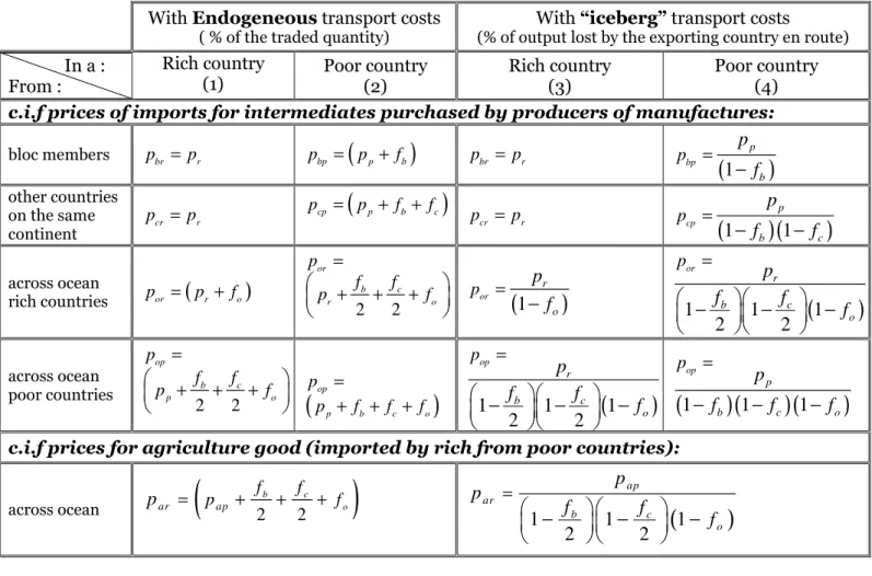
Letting pr p( ) be the producer price in a rich (poor) country, these assumptions on geography and transport costs gives rise to the c.i.f prices reported in table 1. Insert here Table 1: “c.i.f. prices under alternatives transport models”
Table 1 shows that transport costs: (i) increase the prices of foreign intermediate inputs faced by producers of manufactures, and: (ii) increase the difference in relative price of agriculture goods between rich and poor countries which in turn increases the wage gap between rich and poor countries. Tariffs levied on c.i.f. prices.
2.3. Transport Sector with Scale Economies
As mentioned in the introduction, for maritime transport, many trade routes are serviced by a small number of liner companies organized in formal cartels called “liner conferences” (see Hummels, 1999). Moreover, a movement towards concentration has occurred which would not imply market power if transport routes were contestable.9 At least one study, by Fink, Mattoo and Neagu (2002), has found evidence that freight rates are sensitive to regulatory changes meant to constrain collusive behavior by liner conferences, suggesting the exertion of market power. For developing countries, several studies indicate that factors such as national policies which severely restrict competition for transport services have a major influence on the level of freight rates.10
9 Only a dozen firms in the World share 80% of the container traffic (against 40%, 10 years ago).
The two leaders accounting for more than 23% of the traffic, reinforced their domination by taking over hub ports and signing agreements (as the Trans Atlantic Container Agreement) thereby forcing loaders to deal with them (see Rodrigue et al., 2004).
10 For instance, much of Sub-Saharan Africa international transport is cartelized, reflecting the
regulations of African governments intended to promote national shipping companies and airlines. Notably, as described by Amjadi and Yeats (1996) or Collier and Gunning (1999), many African governments (especially West African countries) have adopted “cargoreservation schemes” which allow privileged liner operators to set inflated freight rates considerably above thosethat would prevail in a competitive environment and also to extend inferior quality services.
Modeling the transport sector as a monopoly presents two advantages. First, it captures the monopoly markup often observed in transport service prices on two types of routes: maritime (corresponding to transport between two continental hubs in our framework) and within the South continent.11 Second, investment in new transport technology can be easily introduced explicitly in the model as a function of the shipper’s profit.
As proposed by Hummels and Skiba (2004), I assume that a monopoly shipper takes decisions about how to price transport services and which transport technology to use, maximizing the following profit function,
π
:b b c c o o b c o
f q f q f q C C C
π
= + + − − − (8)With qb, qc, qothe total traded quantities requiring respectively intra-regional, intra-continental and across ocean transport services and C C Cb, c, othe cost functions associated with the production of fb, fc and fo respectively.
Transport costs along a given route
(
h
∈
b c o
, ,
)
decline with the volume of trade along that route by adopting the following Ricardian technology with fixed (or sunk) costs,Fh, and constant marginal costs, κh per unit shipped:{
}
,
; ;
h h h h
C
=
F
+
κ
q
h
=
b c o
(9)To produce transport services, without loss of generality, the monopolist uses labor from the poor country where labor costs are lower. Each transport
technology is characterized by the combination of parameters
{
Fh;κh}
. The initial technology is assumed to require no fixed costs, Fh = , but has a high marginal 0 cost per unit shipped. Then, as trade quantities along a route increase, themonopoly can choose to improve the transport technology used on that route, i.e.
11 Note that the monopoly assumption does not concern transport within the North continent as we
have assumed fb=fc=0 for rich countries. Transport sector for these countries can then be seen as a
to purchase a reduction in marginal cost of ∆
κ
h with an incremental fixed cost Fh, according to the following relation:{
}
, 0,1
, ,
h h hF
=
e
µ κ∆−
µ <=
b c o
(10) In this set-up, changes in technology are discrete12, irreversibleand occur when the profit associated with the new technology overcomes the profit associated with the old one. Note that equation (10) assumes that a given reduction in marginal cost requires greater fixed costs when marginal costs are already small than when marginal costs are high and, to ease interpretation, a given investment generates a similar reduction in marginal costs (µ constant) whatever the selected route h (regional, continental or inter-continental).The parameters entering the cost function in equation (10) are calibrated using estimates in the literature as follows. Start with the most costly technology:
5%
h
κ
=
&F
h=
0
,h
=
{
b c o
, ,
}
. To anticipate results of the simulations reported in section 3 where regional integration starts from an initial situation with a non discriminatory (i.e. MFN) tariff on imports of t=30%, the prices of transport services that maximize the shipper’s profit are the following:, 9.6% b
f = fc =10.1%, fo = 6.5% which implies transport costs in the 10%-20% (of quantity traded) range for a representative poor country (see table 2, column 2). These are in accordance with estimates on the level of transport costs sustained by developing countries (see Limao and Venables, 2001, Hummels, 1999, 2001, Amjadi and Yeats 1996).
Consider now economies of scale. According to remarkably similar econometric estimates for different regions of the world by Hummels and Skiba (2004) and Tomoya and Nishikimi (2002), a 1% increase in trade volume along a route
reduces freight rates by 0.12% percent for all countries on that route. I assume that each investment in new technology induces a gain in marginal cost of 0.2 point of percentage, then determine the value of
µ
(and of the fixed costs) that constrains the monopoly shipper to reduce freight rates charged along a route by around12 As noted by Hummels and Skiba, 2004, “one can think of this choice either as a single yes/no
decision on, for example, port infrastructure or [...] as a menu of ship sizes which the shipper can select”.
0.12% for each 1% increase in trade volume along that route. The value of
µ
that satisfies the preceding constraint is -15. Hence, starting from the initial technology5% h
κ = & Fh =0, the next technology corresponds to a marginal cost of 4.8% requiring a fixed cost around ( 15 )*( 0.2%)
1 0.03
i
F =e − − − = which represents around 10% of the monopoly profit in the initial situation (i.e. under MFN and with the initial technology). Figure 2 illustrates average transport costs for the shipper as a function of distance under this calibration.
Insert here Figure 2: “Evolution of the average cost for the monopoly shipper” 2.4. Equilibrium
Profit, utility maximization and free entry in the production of intermediates lead to a vector of production and consumption in each country and to the
corresponding factor and product prices. Departing from earlier contributions, the model also determines the profit maximizing transport technology by a monopoly shipper (whose profits are symmetrically distributed to the representative
consumer across rich countries) and the corresponding freight rates charges. Given the values of the ad-valorem tariff rate (t), the degree of intra-bloc preference (d), the difference in capital endowment (k) and the parameters
describing preferences, technology for production and transport, together with the wage normalizationwp =1, each equilibrium yields a value for the welfare
indicator of a representative individual in a country. The focus of attention in the remainder of the paper is how individual welfare in a poor country, i.e. Wp, changes under a trade policy organized around a trading bloc relative to a non-discriminatory policy. The full system of equations describing the model is reported in appendix A.1 available upon request.
3. Welfare Implication of Preferential Trade Agreements (PTAs)
We start with welfare implications of PTAs, and then turn to multilateral trade liberalization in section 4. The set-up throughout assumes (C=4), 2 rich and 2 poor ones, with 16 countries per continent (Nr =Np =16). Each continent has 4 regions. I assume that blocs are implemented between the 4 neighbor countries of a region
(B=4). All countries are assumed to levy the same tariff rate of 30% on imports from non member (t=0.3) and to levy an intra-bloc tariff of
t
B=
(
1
−
d t
)
on imports from member countries, where d represents the preference margin within the bloc (0≤d ≤1). Half of consumer income is spent on agricultural goods (α
=0.5) and the elasticity of substitution among intermediate goods,σ
, is equal to 4 (i.e.θ
=0.75).3.1. Traditional “Iceberg” Transport Costs
Since several patterns hold under both endogenous and exogenous transport costs, we start with “iceberg” transport costs. This also helps us relate the results under endogenous transport costs to previous ones which all assumed exogenous
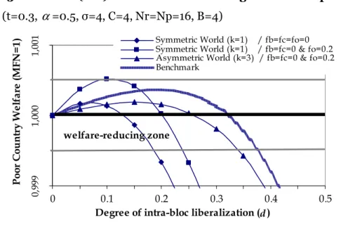
transport costs. Figure 3 (and others) shows how welfare for a representative poor country, i.e. p
W , varies when the preference margin din favor of the regional partner increases. For each set of parameter values, welfare is normalized to 1 under the initial MFN world (W0p =1).
Note first, the inverted U-shape for Wp as preferential margins increase for all configurations and parameter values. This typical second-best result was first noted by Meade (1955) with a slightly different model. Here, as in the Meade model, the marginal benefits from reducing the wedge decrease whereas the marginal costs of creating a wedge by discriminating between trading partners increases.13
Start then with a totally symmetric world
(
k
=
1
)
. This implies that only intra-industry trade occurs between countries (agriculture is not traded as there is no comparative advantage). All countries being identical in terms of economic size, relative factor endowments, trade, tariffs and transport costs, the specification is13 More concretely, the initial reduction in intra-bloc tariffs leads to a small amount of trade
diversion following the shift away from foreign varieties that were consumed in similar proportions for d=0 (and no transport cost). At the same time, trade creation effects are large because domestic varieties (with smaller marginal utility, as they are already consumed in large quantities) are replaced by the bloc members’ varieties. Approaching the last reduction in intra-bloc tariffs (d=1) however, consumption of member and domestic varieties are equalized with a small marginal gain, while the marginal loss of a reduction in foreign varieties is now large: welfare effects of trade creation are then negligible while trade diversion effects are large.
very close to the monopolistically competitive framework in a perfect symmetric world proposed by Frankel, Stein and Wei (1996) and Frankel (1997).
Insert here Figure 3: “Welfare under a PTA with Exogenous Transport Costs”
In the absence of transport costs ( fb = fc = fo =0), p
W reaches a maximum value
(
max)
pW for a degree of bloc preference of around 7% (which implies an
intra-bloc tariff tB =28%) and Wp <W0p for tB =26.2% (d =12.6%). Figure 3 shows that the introduction of positive «iceberg» transport costs changes the relative magnitude of trade creation and trade diversion effects and then maxp
W but does not challenge the overall inverted-U path of welfare. With positive
inter-continental transport costs and zero intra-inter-continental transport costs, relative inter-continental transport costs increase, diminishing the volume of trade with remote countries (on other continents). As expected, reduced trade with remote countries diminishes the costs of implementing sub-continental PTAs and hence also greater utility gains. As shown in figure 3, with fo =0.2, Wp =Wmaxp for
11%
d = and for d >20.2%we face what Frankel et al. (1995) call a “supernatural agreement” to describe a welfare-reducing PTA (i.e. Wp <W0p) among natural partners.
Consider now an asymmetric world
(
k
=
3
)
as in Spilimbergo and Stein (1998). Not surprisingly, the welfare path for a poor country shown in figure 3 is very similar to the path under total symmetry as introducing inter-industry trade with the distant (Northern partner) in effect destroys the positive effects of having lower relative transport costs within the Southern trading bloc. Total welfare costs of discrimination are higher because countries derive utility not only from product differentiation in consumption, but also because of differences in costs.Insert here Table 2: “Transport costs and Welfare under Different scenarios” Figure 3 also reports a simulation with both an asymmetric set-up and non-zero intra-continental transport costs for poor countries. Hence, transport costs are now a function not only of distance but also of the trade partner’s development
level, as described in section 2.2, table 1. This corresponds to our stylized representation of the world and I refer to it as the “benchmark” in the following discussion. I assume fo =0.1 and for poor countries: fb = fc=0.1. Table 2 column 1 reports the corresponding bilateral transport costs derived from the formulas in table 1. As expected from non-zero intra-continental transport costs,14 figure 3 indicates that the negative return of regionalism for a representative poor country sets in later ( p 0p
W <W ford 32%, i.e. tB 20%).
3.2. Endogenous Transport Costs
Traded quantities and transport costs are now jointly determined along the lines described in section 2.3: a monopoly shipper (monopolist for short) jointly chooses profit-maximizing prices and transport technology. The implications of this approach to endogenous transport costs are studied in two steps: in a first step, the monopolist fixes transport service prices with a single transport technology, then in a second step the monopolist jointly chooses prices and transport technology. Figure 4 decomposes the evolution of the welfare indicator as a function of the preferential margin under both scenarios for the same regional PTA considered earlier.
Single transport technology. Under the high-cost single transport technology described in section 2.3, κh =5% & Fh =0, h =
{
b c o, ,}
, the evolution ofp
W appears to be less favorable to PTAs than the one obtained with exogenous “iceberg” costs in section 3.1 (benchmark from figure 3 reported in figure 4) . Tariff reduction, through the reduction of the elasticity of transport demand, causes the monopolist to charge a higher markup over marginal costswhich lowers trade creation, a result also obtained by Hummels and Skiba in partial
equilibrium, the shipper increases his price from 9.6% under MFN (d=0) to 10.2% under FTA (d=1) ).
Insert here Figure 4: “Welfare Implication of PTA with Endogenous Transport Costs”
14 For a detailed discussion of the results with non-zero intra-continental transport costs see
Endogenous Transport Technologies. Figure 4 shows that for the selected parameterization, Wpnever enters the welfare-reducing zone when a regional PTA is implemented. Actually, a “virtuous circle” is generated: the additive intra-bloc trade (due to the decrease in intra-regional tariff) increases the demand for intra-regional transport services which leads the monopolist to adopt lower marginal costs technologies on these routes and then to offer a lower intra-regional freight rate, fb, which in turn boosts intra-bloc trade and positively affects trade creation.15
This optimistic conclusion is partly due to the parameterization which does not impose high sunk cost to obtain marginal transport cost gains. With higher fixed costs per unit decrease in marginal costs, the “jump” to the associated higher welfare curves (the dotted lines in figure 4, normalized to 1 under MFN regime and the first technology could be called iso-technology welfare curves) would occur later. Then, with more costly technologies, poor countries may sometimes and temporarily enter the welfare-reducing zone (until the adoption of the next technology).16
This said, the welfare curve reported in figure 4 is in accordance with the
econometric assessments of economies of scale in transport reported previously. Between MFN
(
d
=
0
)
and a full regional FTA(
d
=
1
)
status, import demand increases by 133% while the price of intra-regional transport services( )
f
bdecreases by around 16% (see table 2 columns 2 and 3). This estimate corresponds to the estimation suggested by the econometric evidence reported earlier, namely that “doubling trade quantities along a route reduces shipping costs by a 12 percent on that route”.
15 Note that intra and inter-continental transport services demands,
c
q and qorespectively,
decrease due to trade diversion. Hence, no new technology is adopted on routes between two regional and two continental hubs respectively. However, as all trade flows have to pass through a regional hub, the improvement on regional routes (and the corresponding decrease in fb)
generates positive externalities for all routes (see table 2 column 3) that mitigate the negative effects of trade diversion.
16
Appendix A.2, available upon request, shows that the results obtained under the set of benchmark parameter values are robust.
4. The Sequencing of Trade Liberalization
I now consider the sequencing issue (or path dependence) of trade liberalization first raised by Bhagwati (1993), recalling than under the traditional exogenous transport cost assumption, reaching free trade under multilateralism or
regionalism would yield the same value. Under the assumption that new transport technologies are not reversed (i.e. sunk costs), columns 4 and 5 in table 2 contrast resulting transport costs under worldwide free trade under the two alternative paths. Column 4 indicates the transport prices charged by the monopolist if worldwide free trade is achieved by the following sequence: first simultaneous implementation of North-North (N-N) and South-South (S-S) FTAs followed by a removal of tariffs between the two resulting blocs. Column 5 reports transport costs when worldwide free trade is reached via multilateral tariff reduction.
Comparing the values of the welfare indicator at the bottom of the table indicates a higher welfare when free trade is achieved under the regional route. This is due to: (i) the adoption of improved transport technologies on intra-regional routes to satisfy increased regional trade resulting from preferential tariff elimination as shown in figure 4; (ii) gains made thanks to the sequencing whereby going to free trade starting with regional free trade only requires developing two routes (intra-continental and inter-(intra-continental) whereas going to free trade multilateral requires spreading transport cost savings on the three routes. 17 As shown at the bottom of the table, of the 0.61%=2.00%-1.39%, 83% (=0.50%/0.61%) of the gain is due to the reduction in transport costs associated with the development of regional routes under regional FTAs.
Hence, with scale economies in transport costs and sunk costs, a symmetric (N-N and S-S) regionalism path to free trade has a persistent effect on trade flows through a permanent effect on regional transport costs that improves poor country welfare compared with the alternative multilateral path, i.e.
(
WNN SSFT, >WMFNFT)
. As part of sensitivity analysis, next section explores an alternative path with the implementation of North-South (N-S) FTAs.
5. Extensions
Independent transport routes. As an alternative to the “hub-and-spoke” transport network structure, I now assume that each country operates under three
independent routes, each corresponding to one of the three kinds of trade partners: regional, continental outside the region and across ocean. It turns out that the patterns discussed here are robust to this alternative modeling of
transports as far as only the regional routes are concerned. There is no significant difference between the two transport structures during the implementation of an FTA.18 Concerning the multilateral liberalization stage, this conclusion is strongly reinforced: with an “independent routes” network, Wp under FTA (but no
worldwide liberalization) is superior to Wp under worldwide free trade reached from a MFN situation! Actually, with a multilateral liberalization from a MFN situation (with t=30%), trade is spread too thinly among all partners so that the improved shipping technology is never adopted.
North-South Regional Blocs. As first noted by de Melo and Panagariya (1993), the distinguish feature of the current wave of regionalism is that it is now N-S (rather than N-N and S-S during the first wave of regionalism in the 1960s). Figure 5 contrasts welfare under N-S regionalism with welfare under S-S/N-N considered earlier. The evolution of p
W during the N-S bloc implementation (i.e. bloc between two poor and two rich countries) is close to the evolution of Wp under multilateral liberalization (but with still the inverted U-shape) as now the two sources of gains from trade, product variety and costs differences can be exploited within the bloc.
Insert here Figure 5: “Symmetric vs. Asymmetric Trade Blocs”
In terms of reduced transport costs, symmetric blocs lead to a gain of 2% in regional marginal transport costs, whereas N-S blocs, in promoting trade on the 3 routes (regional, continental, across ocean), lead to gains that are spread out over the 3 routes (gain of 1% on each marginal transport cost, which is smaller than under worldwide free trade).
As far as multilateral liberalization is concerned, Wp under worldwide free trade when reached through N-S regionalism is (i) higher than through MFN
liberalization (thanks to higher volume of trade and then better technology on all 3 routes) but (ii) smaller than through symmetric blocs due to less advanced
regional transport technology (which is the base of all kinds of transport costs in our model). Then, the ranking of paths towards Free Trade, for the representative parameterization adopted here, the asymmetric bloc approach yields a welfare gain of an elimination of protection in-between the alternatives examined earlier, i.e.
(
WNN SSFT, >WNSFT >WMFNFT)
.6. Conclusions
This paper has challenged the pessimistic view that RTAs between neighbor developing countries are likely to be welfare-reducing. South-South trade agreements look more favorable once one takes into account scale economies in transport (and the associated changes in transport technology from a profit-maximizing monopoly shipper). For plausible parameter values, a Southern country’s welfare never enters in a welfare-reducing zone when an FTA is implemented with a Southern regional partner as a “virtuous circle” is set in motion: preferential trade reduces intra-regional transport costs, which in turn boosts intra-bloc trade leading to trade creation. A regional approach to trade liberalization may also be preferable to a multilateral approach in the presence of irreversible effects in terms of investments in regional transport technologies.
While these results are at best suggestive, they provide support to several recent RTAs. For example, the Economic Partnership Agreements (EPAs) currently under negotiation between the EU and ACP involve a North-South FTA built upon a prior South-South FTA. More directly, the New Partnership for Africa’s
Development (NEPAD) puts emphasis on investments in regional infrastructure and transport networks. Likewise, many South-South RTAs (e.g. MERCOSUR, Andean pact, SADC, COMESA, UEMOA) have included “transport and trade facilitation” agreements as part of their regional integration initiatives. The challenge is to quantify these beneficial channels of regional integration with greater accuracy.
References
Amjadi, A. and A. Yeats. 1996. "Have Transport Costs Contributed to the Relative Decline of Sub-Saharan African Exports? Some Preliminary Empirical Evidence”. Policy Research Working Paper #1559, World Bank, Washington DC.
Anderson, J. and E. van Wincoop. 2004. “Trade Costs” Journal of Economic Literature. Vol. 42, No. 3 (September),191-751.
Baier, S. L., and J. Bergstrand. 2004. “On the Economic Determinants of Free Trade Agreements” Journal of International Economics, Vol 64, No. 1, October, 29-63.
Bhagwati, J. 1993. “Regionalism and Multilateralism: an Overview.” In J. de Melo and A. Panagariya eds., New Dimensions in Regional Integration, Oxford Univ. Press.
Busse, M., 2003. “Tariffs, Transport Costs and the WTO Doha Round: The Case of Developing Countries”, Journal of International Law and Trade Policy, Vol. 4, No. 1, 15-31.
Clark, X., Dollar, D. and A. Micco, 2002. “Maritime Transport Costs and Port Efficiency”. Policy Research Working Paper #2781, World Bank, Washington DC. Collier, P. and J. W. Gunning. 1999. "Explaining African Economic Performance" Journal of Economic Literature. Vol. XXXVII (March), 64-111.
Djankov, S., Freund C.L. and C.S. Pham. 2006. “Trading on Time”. World Bank Policy Research Working Paper N°3909.
Fink, C., Mattoo A. and I.C. Neagu. 2002. “Trade in International Shipping Services: How Much Does Policy Matter?” World Bank Economic Review. Vol. 16 No. 1, 88-108.
Frankel, J. A., Stein, E. and S-J Wei. 1996. “Regional Trading Arrangements: Natural or Supernatural?” American Economic Review (AEA Papers and Proceeding), May, vol. 86, no. 2, 52–56.
Frankel, J. A. 1997. Regional Trading Blocs in the World Economic System. Institute for International Economics, Washington, DC.
Freund. C. 2000. “Different Paths to Free Trade: The Gains from Regionalism”, Quarterly Journal of Economics, vol. 115, no. 4, 1317-1341.
Fujita, M., Krugman, P.R., Venables, A.J., 1999. The Spatial Economy: Cities, Regions and International Trade. MIT Press, Cambridge.
Hummels, D. 1999. “Have International Transportation Costs Declined?” Mimeo. Graduate School of Business. University of Chicago (November).
Hummels, D. and Skiba, A. 2004. “A Virtuous Cycle? Regional Tariff
Liberalization and Scale Economies in Transport”, In A. Estevadeordal, D. Rodrik, A. M. Taylor and A. Velasco, ed., FTAA and Beyond: Prospects for Integration in the America. Harvard University Press.
Krugman, P. 1991a. “Is Bilateralism Bad?” in E. Helpman and A. Razin, eds., International Trade and Trade Policy. Cambridge, MA: MIT Press, 9–23. Krugman, P. 1991b. “The Move to Free Trade Zones” in Policy Implications of Trade and Currency Zones, a symposium sponsored by the Federal reserve Bank of Kansas City.. Kansas City, KS.
Krugman, P. 1998. “Comment on ‘Continental Trading Blocs: Are They Natural or Supernatural?’ ” In J. A. Frankel, ed., The Regionalization of the World Economy. Chicago: University of Chicago Press, 114–15.
Limao, N. and A. Venables. 2001. “Infrastructure, Geographical Disadvantage, Transport Costs and Trade”. World Bank Economic Review. Vol. 15: 451-479. Meade, J. E. 1955. The Theory of Customs Unions. Amsterdam: North-Holland. Melo, J. de and A. Panagariya (1993) “Introduction” in J. de Melo and A. Panagariya eds. , New Dimensions in Regional Integration, Oxford Univ. Press.
Panagariya, A. 1998. "Do transport Costs Justify Regional Preferential Trading Arrangements? No". Weltwirtschaftliches Archiv, Vol. 134 (2), 280-301.
Rodrigue, J-P, Comtois C., Kuby M. and B. Slack (2004) Transport Geography on the Web, Hofstra University, Department of Economics & Geography,
http://people.hofstra.edu/geotrans.
Samuelson, P. 1954. “The Transfer Problem and Transport Costs”. The Economic Journal, Vol. 64, 264-289.
Spilimbergo, A. and E. Stein. 1998. “The Welfare Implications of Trading Blocs among Countries with Different Endowments” In J. A. Frankel, ed., The
Regionalization of the World Economy. Chicago: University of Chicago Press, 121– 45.
Tomoya M. and K. Nishikimi. 2002. “Economies of transport density and
industrial agglomeration”. Regional Science and Urban Economics 32, 167-200. UNCTAD. 2003. Review of Maritime Transport. http://www.unctad.org/. Viner, J. 1950. The Customs Union Issue. New York: Carnegie Endowment for International Peace.
Wonnacott, P. and M. Lutz. 1989. “Is There a Case for Free Trade Areas?” In J. Schott, ed., Free Trade Areas and U.S. Trade Policy. Washington, D.C.: Institute for International Economics.
Table 1: “c.i.f. prices under alternatives transport models” With Endogeneous transport costs
( % of the traded quantity)
With “iceberg” transport costs
(% of output lost by the exporting country en route)
In a : From : Rich country (1) Poor country (2) Rich country (3) Poor country (4) c.i.f prices of imports for intermediates purchased by producers of manufactures:
bloc members pbr = pr pbp =
(
pp + fb)
pbr = pr(
1)
bp p b p p f = − other countries on the same continent cr r p = p pcp =(
pp + fb+ fc)
cr r p = p(
1)(
1)
cp p b c p p f f = − − across ocean rich countries por =(
pr + fo)
2 2 or b c r o p f f p f = + + + or(
1
)
r o pp
f
=−
1
1
(
1
)
2
2
or r b c o pp
f
f
f
=
−
−
−
across ocean poor countries 2 2 op b c p o p f f p f = + + + (
opp b c o)
p p f f f = + + + 1 1(
1)
2 2 op r b c o p p f f f = − − − (
1
)(
1
)(
1
)
op p b c o pp
f
f
f
=−
−
−
c.i.f prices for agriculture good (imported by rich from poor countries):
across ocean
(
2 2)
b c o ar ap f f p f p = + + +(
)
1 1 1 2 2 ap ar b c o p p f f f = − − − Table 2:”Transport costs and Welfare under Different scenarios” ( k=3,
α
=0.5, σ=4, C=4, Nr=Np=16, B=4)Iceberg Endogenous Transport costs
Bench- MFN FTA Worldwide FT
-mark Via FTA Via MFN
Column (1) (2) (3) (4) (5)
Transport costs on each route
intra-regional fb 10.0% 9.6% 8.0% 7.8% 7.8%
intra-continental fc 10.0% 10.1% 10.2% 7.9% 8.3%
inter-continental fo 10.0% 6.5% 6.4% 4.8% 5.2%
Transport costs between :
2 poor countries-same bloc 10.0% 9.6% 8.0% 7.8% 7.8%
2 poor countries-same continent 19.0% 19.7% 18.2% 15.6% 16.1% 2 poor countries-different continents 27.1% 26.2% 24.7% 20.4% 21.3% 1 poor country and 1 rich country 18.8% 16.4% 15.6% 12.6% 13.3% 2 rich countries-same continent 0.0% 0.0% 0.0% 0.0% 0.0% 2 rich countries-different continents 10.0% 6.5% 6.4% 4.8% 5.2% Increase in p
Figure 1: “Hub-and-Spoke” transport network
(2 continents, 4 regions by continent, 4 countries by region)
Figure 2: “Evolution of the average cost for the monopoly shipper”
4,50% 4,60% 4,70% 4,80% 4,90% 5,00% 5,10% 100 110 120 130 140 150 160 170
quantity traded along a route (base 100 with the first technology)
Average cost 5% & 0 h Fh
κ
= = 4.8% & 0.031 h Fhκ
= = 4.6% & 0.062 h Fhκ
= = 4.4% & 0.094 h Fhκ
= = 4.2% & 0.127 h Fhκ
= = 4.0% & 0.162 h Fhκ
= = 3.8% & 0.197 h Fhκ
= =Figure 3: “Welfare (Wp) under a PTA with Exogenous Transport Costs” (t=0.3, α=0.5, σ=4, C=4, Nr=Np=16, B=4) 0, 99 9 1, 00 0 1, 00 1 0 0.1 0.2 0.3 0.4 0.5
Degree of intra-bloc liberalization (d )
P o o r C o u n tr y W e lf a re ( M F N = 1
) Symmetric World (k=1) / fb=fc=fo=0
Symmetric World (k=1) / fb=fc=0 & fo=0.2 Asymmetric World (k=3) / fb=fc=0 & fo=0.2 Benchmark
welfare-reducing zone
Figure 4: “Welfare Implication of PTA with Endogenous Transport Costs” (t=0.3, k=3,
α
=0.5, σ=4, C=4, Nr=Np=16, B=4)Figure 5: “Symmetric vs. Asymmetric Trade Blocs” (t=0.3, k=3,
α
=0.5, σ=4, C=4, Nr=Np=16, B=4) 0, 99 8 1 ,0 0 0 1, 00 2 1 ,0 0 4 1, 00 6 0 0.1 0.2 0.3 0.4 0.5 0.6 0.7 0.8 0.9 1 Degree of intra-bloc liberalization (d )P o o r C o u n tr y W e lf a re ( M F N = 1 )
Benchmark (Iceberg Transport Costs) Single Transport Technology Endogenous Transport Technologies
welfare-reducing zone 1 ,0 0 0 1 ,0 0 6 1 ,0 1 2 1 ,0 1 8 0 0.1 0.2 0.3 0.4 0.5 0.6 0.7 0.8 0.9 1 P o o r C o u n tr y W e lf a re ( M F N = 1 ) blocs "S-S" & "N-N" blocs "N-S"
APPENDIX A.1.MODEL EQUATIONS
As describe in section 2, we assume: (i) 3 sectors:
Agriculture, produced with labor under constant returns to scale;
Intermediate good, produced with capital under increasing returns to scale; Manufactures, produced with intermediate good under constant returns to scale;
(ii) 2 types of countries, with a capital to labor ratio of 1 in the poor country and of k>1 in the rich country;19
(iii) a World of 4 continents (C=4), 2 continents of rich countries and 2 continents of poor ones, 16 countries per continent (Nr =Np =16); Each continent comprises 4
regions; We assume that blocs are implemented between the 4 neighbor countries of a same region (B=4);
(iv) a “hub-and-spoke” transport network with 3 types of freight rates: fb: intra-regional (from spoke to spoke via the regional hub);
fc: intra-continental (from a regional hub to another via the continental hub); fo: intercontinental (from a continental hub to another);
Optimization Problem of Intermediate Input Producers
{
}
, 1.. ;
ji
p ji ji ji ji i i
Max π = p x −K r j= n i= r p
With πji the producer profit of the jth variety in country i,
ji
x (pji) the production (producer price) of the jth variety in country i ,
i
n the number of intermediate input varieties produced in country i and ri the price of capital in country i. Intermediate inputs are produced under monopolistic competition with capital. The total amount of capital used in the production of the jth variety in country i,
ji
K , is: Kji =γ +βxji with γ the fixed cost and β the constant marginal cost.
From the first order condition for profit maximization (derivation available upon request) we obtain the profit-maximizing price:20
{
}
, 1.. i ; i ji i j n i r p p β r p θ = = = = (A.1)which, combined with the free entry condition, gives the output per variety:
{
}
, 1.. ; (1 ) ji i i x x θγ j n r p β θ = = = = − (A.2)19 For simplicity we assume that labor, L, also represents the population size and that 1
r p
L =L = . The total capital is therefore Kr =kLr =k in a rich economy and Kp =Lp = in a poor one. 1
Introducing the expression of x into the capital market equilibrium condition of a country i, i.e.
(
)
(
)
1 1 i i n n i ji ji i j j j K K βx γ n βx γ = ==
∑
=∑
+ = + , gives the number of varieties produced in country i:(
)
{
}
1 , ; i i i K n θ r p γ = − = (A.3)Equation (A.3) implies that the number of varieties produced in the rich country will be larger than in poor countries by a factor of k:
r p r p n k n
K
K
==
(A.4)The relative price of capital in rich and poor countries will be denoted as
ρ
. Hence, according to equation (A.1), ρ is also equal to the price of the home varieties in a rich country, pr, relative to that of the home varieties in a poor countries, pp:r r
p p
r p
r = p =ρ (A.5)
Optimization Problem of Final Good Producer
The prices of foreign intermediate inputs faced by producers of manufactures, in terms of the ones produced at home, are given by:
In a rich country:
(
)
(
)
(
)(
)
(
)
(
)
1 (1 ) 1 1 1 1 1 2 2 2 2 br r cr r or r o b c r b c o op p o p p p p p d t p p t p p f t f f p f f f p p f t t p p p ρ = + − = + = + + = + + + + = + + + +
(A.6r) In a poor country(
)
(
)
(
)
(
)
(
)
(
)
(
)
(
)
1 (1 ) 1 1 1 1 1 2 2 2 2 bp p b cp p b c op p b c o b c b c o or r o p r r r p p f d t p p f f t p p f f f t f f f f f p p f t p t p p p ρ = + + − = + + + = + + + + = + + + + = + + + + (A.6p)with origin r: rich country/ p: poor country/ b: bloc members/ c: other countries (non members) within the continent/ o: overseas countries;
t represents the MFN ad valorem tariff (uniform across countries);
d represents the degree of intra-bloc liberalization [d=1 (0) free trade area (MFN)]. The producer of the final good faces the following problem:
In a rich country
(
)
{
1 0 1 . . ( 1) ( ) 1 2 mr i r r r r br br r r cr cr r r or or Max q c s t n c p B n c p N B n c p C N n c p θ θ θ = < ≤ + − + − +
−
∑
14243
14
4244
3
home varieties varieties from bloc members varieties from other countries of the continent
varieties from rich cou
2 p p op op mr mr C N n c p q p + ≤
1442443
14243
varieties from poor countries ntries overseas In a poor country
(
)
1 . . ( 1) ( ) 1 2 mp i p p p p bp bp p p cp cp p p op op Max q c s t n c p B n c p N B n c p C N n c p θ θ = + − + − + − ∑
123 1442443 1442443home varieties varieties from bloc members varieties from other countries of the continent
varieties from poor cou
2 r r or or mp mp C N n c p q p + ≤
14442444ntries overseas3 14243varieties from rich countries
with ci the consumption of an intermediate good variety produced in country i.
Then, the producer of manufactures will demand the following relative quantities of intermediate inputs (from the first order conditions, derivation available upon request):
In a rich country
{
}
1 1 ; ; ; r i r i p c c p with i cr br or op θ − = = (A.7r) In a poor country{
}
1 1 ; ; ; p i p i p c c p with i cp bp op or θ − = = (A.7p)In equilibrium, the per capita production of the manufactured good will be: In a rich country: