HAL Id: hal-01313404
https://hal.archives-ouvertes.fr/hal-01313404v2
Preprint submitted on 12 Dec 2016
HAL is a multi-disciplinary open access
archive for the deposit and dissemination of
sci-entific research documents, whether they are
pub-lished or not. The documents may come from
teaching and research institutions in France or
abroad, or from public or private research centers.
L’archive ouverte pluridisciplinaire HAL, est
destinée au dépôt et à la diffusion de documents
scientifiques de niveau recherche, publiés ou non,
émanant des établissements d’enseignement et de
recherche français ou étrangers, des laboratoires
publics ou privés.
Distributed under a Creative Commons Attribution| 4.0 International License
Learning stochastic eigenvalues
Roman Andreev
To cite this version:
ROMAN ANDREEV†
Abstract. We train an artificial neural network with one hidden layer on realizations of the first few eigenvalues of a partial differential operator that is parameterized by a vector of independent random variables. The eigenvalues exhibit “crossings” in the high-dimensional parameter space. The training set is constructed by sampling the parameter either at random nodes or at the Smolyak collocation nodes. The performance of the neural network is evaluated empirically on a large random test set. We find that training on random or quasi-random nodes is preferable to the Smolyak nodes. The neural network outperforms the Smolyak interpolation in terms of error bias and variance on nonsimple eigenvalues but not on the simple ones.
1. The stochastic eigenvalue problem
In this note we compare the out-of-sample prediction of the Smolyak sparse grid interpolant with that of a simple artificial neural network for a stochastic eigenvalue problem. Our model problem is the parametric partial differential eigenvalue problem
−∇ · (c(x, y)∇u(x, y)) + u(x, y) = λ(y)u(x, y), x ∈ D, y ∈ Y, (1)
where D := (−1, 1)2 is the spatial domain and Y := [0, 1]M is the parameter space. We impose
homogeneous Neumann spatial boundary conditions. The conductivity coefficient has the form c(x, y) := 1 +PM
m=1ψm(x)ym.
(2)
We think of the ym∈ [0, 1] as independent uniformly distributed random variables. Throughout,
the stochastic dimension is M = 16 and the ψm are the indicator functions of the subdomains
obtained by partitioning the spatial domain into 4 × 4 equal parts. The problem (1) will be discretized with P1 finite elements with 422 unknowns using the Matlab PDE toolbox.
Our quantity of interest is the set of the first 9 eigenvalues,
QI(y) := {1 = λ1(y) ≤ λ2(y) ≤ . . . ≤ λ9(y)}.
(3)
For y = 0, the nontrivial ones are
λ2,3= 0+14 π2+ 1, λ4= 1+14 π2+ 1, λ5,6 =0+44 π2+ 1, λ7,8= 1+44 π2+ 1, λ9= 4+44 π2+ 1,
and the last one is simple.
yA yB 0 5 10 15 20 #1 #2,3 #4 #5 #6 #7 #8
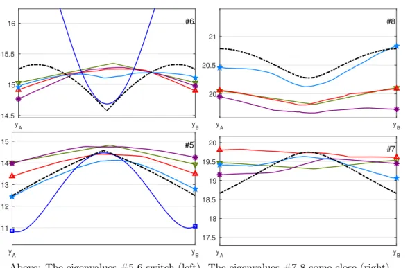
However, as we vary the parameter, the eigenvalues split, leading to a nonsmooth (Lipschitz) dependence on the parameter. For example (figure on the right and Fig-ure 1), interpolating linearly between c(·, yA) = 1 +1x1>0 and c(·, yB) = 1 +1x2>0, the eigenvalues #2–3 remain almost identical (slight discretization asymmetry), #5–6 switch midway, while #7–8 (and also #9) remain distinct. These eigenvalue “crossings” or “switchings” make it diffi-cult to capture the parameter dependence over the whole high-dimensional parameter space.
In the next section we discuss two regression methods for that purpose, both based on sampling in the parameter domain: Smolyak interpolation and artificial neural networks.
Date: December 12, 2016.
2010 Mathematics Subject Classification. 15B51, 35R60, 62M45, 62M40, 65N25, 65N30, 65Y05, 65Y20, 68T37. Key words and phrases. uncertainty quantification, stochastic eigenvalues, neural networks, sparse grids.
LEARNING STOCHASTIC EIGENVALUES 2
2. Two regression methods
2.1. The Smolyak interpolant [2]. For each integer level ` ≥ 0 let i`be a univariate interpolation
operator on the interval [0, 1]. We will use the polynomial interpolation operator based on the Clenshaw–Curtis nodes
N0= {12} and N`= {12(1 − cos(2−`kπ)) : 0 ≤ k ≤ 2`}, ` ≥ 1.
(4)
For a multiindex set Λ ⊂ NM
0 , the multivariate Smolyak interpolation operator IΛ is defined by
IΛ:=Pν∈Λ(jν1⊗ jν2⊗ . . . ⊗ jνM), (5)
where j`:= i`− i`−1 is the univariate increment and i−1:= 0. We confine the discussion to the
multiindex sets of a given total level L ≥ 0, ΛL:= {ν ∈ NM0 :
P
mνm≤ L},
(6)
and write IL for the resulting multivariate Smolyak interpolation operator. This multiindex set
is monotone: if µ ∈ ΛL and if ν ≤ µ coordinatewise then also ν ∈ ΛL. This, and the nestedness
property N`−1 ⊂ N` of the Clenshaw–Curtis nodes imply the unisolvency of the multivariate
interpolation operator on the sparse grid (observe the redundancy in the union) NL:=Sν∈ΛL(Nν1× Nν2× . . . × NνM) ⊂ Y,
(7)
because the number of collocation nodes in (7) matches the dimension of the range of the inter-polation operator (5). With M = 16 stochastic dimensions, the number of collocation nodes is #N0= 1, #N1= 33, #N2= 545, #N3= 60049, etc. We write
Sm[L] := IL◦ QI : RM → R9
(8)
for the interpolated quantity of interest.
2.2. Artificial neural networks. We consider the simple class of neural networks of the form input (M parameters)linear−→ ReLU (H hidden units)linear−→ output (9 real values), (9)
or as the composition
NN : RM → R9, NN = (h 7→ Ch + c) ◦ ReLU ◦ (y 7→ By + b),
(10)
with the (9(H + 1) + H(M + 1)) learnable parameters
{C ∈ R9×H, c ∈ R9} = 2nd all-to-all layer, {B ∈ RH×M, b ∈ RH} = 1st all-to-all layer. (11)
The “rectified linear unit” is the function ReLU : x 7→ max{x, 0}, acting componentwise when applied to a vector. The number of “hidden units” will be H ∈ {M, 4M, 16M }.
A training set or a test set is a collection of reference nodes N ⊂ Y together with the precomputed values of the quantity of interest (3) at those nodes. We refer to a pair (y, QI(y)) as a sample. We consider two types of reference nodes for training the neural network:
(1) the Smolyak collocation nodes NL from (7), and
(2) randomly generated nodes eNL of the same cardinality as NL.
The random training set is generated only once for each level L and used for all configurations. By “average” we will mean the ensemble average over the training set or over the test set.
The learnable parameters are initialized uniformly at random from [−s, s] where s = 1/√M for the first linear layer and s = 1/√H for the second one. Then, they are trained in 10k iterations of stochastic gradient descent. Each iteration is a pass over the training set in random order; for each sample (y, q), the learnable parameters α are adjusted (all at once) by the gradient scheme
α ← α − r∂α∂ D(q, NN(y)), D(q, p) := 19|q − p|1,
(12)
where r > 0 is the learning rate (initially, r = 0.1) and | · |1 is the vector 1-norm measuring the
prediction discrepancy. The derivatives of ReLU and | · |1are right-continuous. After each iteration,
the learning rate is set to 1% of the average prediction discrepancy. The input/output data are offset by their average during the training phase. We write NN[H, N ] for the neural network with H hidden units trained on the node set N . We use the torch7 environment for the training.
3. Evaluation
Given a predictor P = (8) or P = (10), we evaluate its quality over a fixed test set of 100k samples on random test nodes Ntest⊂ Y . The average and the standard deviation of the eigenvalues in the
test set are as follows (rounded to two postcomma digits):
eigenvalue: #1 #2 #3 #4 #5 #6 #7 #8 #9
average 1 4.55 4.68 8.24 5.24 15.47 18.77 19.62 29.6
std dev 0 0.2 0.2 0.39 0.74 0.73 0.97 0.98 1.47
Predictions along a non-axiparallel segment in the parameter space are shown in Figure 1. We examine the errors
δk(y) := (QI(y) − P(y))k, y ∈ Ntest,
(13)
in the prediction of the k-th eigenvalue. Unsorted predictions occurred at the following rates: Sm[L] NN[M, NL] NN[4M, NL] NN[M, eNL] NN[4M, eNL]
L = 2 71.5% 3% 0.6% 0.31% 1.3%
L = 3 63.5% 2.8% 0.15% 0.02% 0.01%
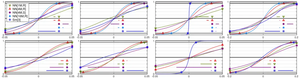
We call the average ¯δk of δk the prediction bias. Figures 2–3 show the empirical cumulative
distribution function of the bias-free prediction error (δk− ¯δk) along with the prediction bias ¯δk for
different predictors. We observe the following (recall, M = 16 is the stochastic dimension): (1) For the nonsimple eigenvalues #2, 3, 5, 6, 7, 8, the neural network NN[4M, eNL] trained on
random nodes performs consistently better in terms of the prediction bias and prediction error variance than the Smolyak interpolation operator Sm[L].
(2) This behavior is reversed for the simple eigenvalues #4 and #9. This is explained by the analytic dependence of simple eigenvalues on the parameter [1]. Increasing the number of hidden units from H = 4M to H = 16M is still not sufficient to surpass interpolation. (3) Training the neural network on the Smolyak nodes as opposed to random nodes clearly
decreases the prediction accuracy.
(4) The neural network with M hidden units instead of 4M is less competitive on training level L = 3 than on L = 2.
(5) The results are essentially the same for the quasi-random Sobol points (as generated by the Matlab command sobolset(M)) instead of the random ones (not shown).
Finally, we note that neural networks and sparse grid interpolation have different distributions of offline/online costs. While the offline training of the neural network is lengthy, the online prediction is much quicker than sparse grid interpolation, especially for high-dimensional parameters. However, both effects can be offset by parallelization.
Acknowledgment
Supported by the Swiss NSF Advanced Postdoc.Mobility grant #164616. References
[1] Roman Andreev and Christoph Schwab. Sparse tensor approximation of parametric eigenvalue problems. In Ivan G. Graham, Thomas Y. Hou, Omar Lakkis, and Robert Scheichl, editors, Numerical Analysis of Multiscale Problems, volume 83 of Lecture Notes in CSE, pages 203–241. Springer Berlin Heidelberg, 2012. 3
[2] Sergey A. Smolyak. Quadrature and interpolation formulas for tensor products of certain classes of functions. Sov. Math. Dokl., 4:240–243, 1963. 2
†
Université Paris Diderot, Sorbonne Paris Cité, LJLL (UMR 7598 CNRS), F-75205, Paris, France E-mail address: [email protected]
LEARNING STOCHASTIC EIGENVALUES 4 y A yB 14.5 15 15.5 16 #6 y A yB 20 20.5 21 #8 y A yB 11 12 13 14 15 #5 yA yB 17.5 18 18.5 19 19.5 20 #7
Above: The eigenvalues #5-6 switch (left). The eigenvalues #7-8 come close (right). The Smolyak interpolant for #7-8 is outside the range shown.
y A yB 4 4.1 4.2 4.3 4.4 4.5 4.6 #2 Exact NN[1M,R] NN[4M,R] NN[4M,S] NN[16M,R] Sm[3] y A yB 4.4 4.5 4.6 4.7 4.8 #3
Above: The eigenvalues #2-3 are slightly distinct (due to discretization asymmetry).
y A yB 8 8.1 8.2 8.3 #4 y A yB 27 28 29 30 31 #9
Above: The simple eigenvalues #4 and #9. Eigenvalue #9 comes close to #10 midway.
Figure 1. Exact and predicted eigenvalues along the parameter space segment from c(·, yA) = 1 +1x1>0 to c(·, yB) = 1 +1x2>0. See #2 for the annotation.
LEARNING STOCHASTIC EIGENV ALUES 5 -0.050 0 0.05 NN[1M,R] NN[4M,R] NN[4M,S] NN[16M,R] Sm[3] -0.05 0 0.05 0 -0.05 0 0.05 0 -0.2 0 0.2 0 -0.05 0 0.05 0 1 -0.05 0 0.05 0 1 -0.05 0 0.05 0 1 -0.2 0 0.2 0 1
Figure 2. The empirical cumulative distribution function of the bias-free prediction errors for the eigenvalues #2, 3, 4, 5 (left to right). The prediction bias is shown as the bar in the lower right corner. Training levels L = 3 (top) and L = 2 (bottom).
-0.20 0 0.2 1 NN[1M,R] NN[4M,R] NN[4M,S] NN[16M,R] Sm[3] -0.8 0 0.8 0 1 -0.8 0 0.8 0 1 -0.2 0 0.2 0 1 -0.2 0 0.2 0 1 -0.8 0 0.8 0 1 -0.8 0 0.8 0 1 -0.2 0 0.2 0 1