Ethnic Unemployment Rates and Frictional Markets

(1)

HAL Id: halshs-00849074

https://halshs.archives-ouvertes.fr/halshs-00849074

Preprint submitted on 30 Jul 2013

HAL is a multi-disciplinary open access

archive for the deposit and dissemination of

sci-entific research documents, whether they are

pub-lished or not. The documents may come from

teaching and research institutions in France or

L’archive ouverte pluridisciplinaire HAL, est

destinée au dépôt et à la diffusion de documents

scientifiques de niveau recherche, publiés ou non,

émanant des établissements d’enseignement et de

recherche français ou étrangers, des laboratoires

Ethnic Unemployment Rates and Frictional Markets

Laurent Gobillon, Peter Rupert, Etienne Wasmer

To cite this version:

Laurent Gobillon, Peter Rupert, Etienne Wasmer. Ethnic Unemployment Rates and Frictional

Mar-kets. 2013. �halshs-00849074�

(2)

WORKING PAPER N° 2013 – 26

Ethnic Unemployment Rates and Frictional Markets

Laurent Gobillon

Peter Rupert

Etienne Wasmer

JEL Codes: R23, E24

Keywords: Discrimination, Ethnic groups, Local markets, Matching models

P

ARIS

-

JOURDAN

S

CIENCES

E

CONOMIQUES

48, BD JOURDAN – E.N.S. – 75014 PARIS TÉL. : 33(0) 1 43 13 63 00 – FAX : 33 (0) 1 43 13 63 10

(3)

1

Ethnic Unemployment Rates and Frictional Markets

∗

Laurent Gobillon

INED and PSE

Peter Rupert

University of California, Santa Barbara

Etienne Wasmer

Sciences-Po Paris and LIEPP

June 22, 2013

Abstract

The unemployment rate in France is roughly 6 percentage points higher for African immigrants than for natives. In the US the unemployment rate is approximately 9 percentage points higher for blacks than for whites. Commute time data indicates that minorities face longer commute times to work, potentially reflecting more difficult access to jobs. In this paper we investigate the impact of spatial mismatch on the unemployment rate of ethnic groups using the matching model proposed byRupert and Wasmer(2012). We find that spatial factors explain from 1 to 1.5 percentage points of the unemployment rate gap in both France and the US, amounting to 17% to 25% of the relative gap in France and about 10% to 17.5% in the US. Among these factors, differences in commuting distance play the most important role. In France, though, longer commuting distances may be mitigated by higher mobility in the housing market for African workers. Overall, we still conclude that labor market factors remain the main explanation for the higher unemployment rate of Africans.

∗_{We thank Jean-Baptiste Kerveillant for excellent research assistance. We are also grateful to Gilles Duranton, Morgane Laouenan,} Bruno Van der Linden, the participants of the II Workshop on Urban Economics in Barcelona and the IRES Research Seminar in Louvain-la-Neuve, as well as two anonymous referees for their useful comments.

(4)

1 Introduction

The persistence of the unemployment rate gap between natives and immigrants, or in the US context between whites and blacks, is a major policy concern. However, there is still debate whether it is “race” or “space” that is the key explanatory factor of the poor labor market outcomes of many minorities (seeEllwood,1986). The spatial mismatch literature, initiated byKain(1968), has indeed attempted to determine whether minority workers have worse access to the labor market or whether they face barriers in housing choice, making it difficult to locate close to job opportunities.

In this paper we propose a methodology to assess the “dynamic spatial mismatch” hypothesis, that is, the intertemporal decisions of housing, commuting, job acceptance and quits. We develop and quantify a tractable macro-economic matching model to assess the importance of job market factors and spatial factors. Our contribu-tion is threefold: we model friccontribu-tions on both the labor and housing markets whereas, in the literature, friccontribu-tions are usually introduced only in one market; we calibrate the model to get quantitative results rather than giving only theoretical predictions; finally, we perform comparative statics to assess the contribution of job and spatial factors to the ethnic unemployment rate gap.

There are several forces possibly at work that have been formulated in the literature. Minority workers may not have the same access to jobs due to differences in unobservables related to productivity or discrimination in the labor market. Employers may have racial preferences and discriminate (Becker,1971). They may also consider minority workers to be, on average, less productive and assign their average productivity to all minority applicants if productivity is not observed during the recruitement process (Phelps,1972). Finally, they may avoid employing minority workers because they expect their customers to be reluctant interacting with them (Borjas and Bronars,

1989;Combes et al.,2011).

According to the spatial mismatch literature, housing market discrimination may prevent US black workers from locating close to job centers and the resulting distance to job opportunities could be a cause of their unemployment.1

Zax and Kain(1996) investigates the effect of the relocation of a plant in Detroit from the city center to a white

neighborhood, where housing discrimination against blacks is considered to be operational, on quits and residential relocations of black and white workers. They show that blacks quit more often and relocate less often close to

1_{For empirical surveys on spatial mismatch, see}_{Jencks and Mayer}₍₁₉₉₀_),_Kain₍₁₉₉₂_),_{Ihlanfeldt and Sjoquist}₍₁₉₉₈_{) and}_Hellerstein

(5)

the plant. We consider in our model that there is a Minority (here, non-natives, predominantly Africans) and a Majority, with the Minority have housing opportunities which are possibly associated to longer commuting distances during the residential search process.

The effect of distance on unemployment has been investigated in the theoretical literature mostly in an urban economics setting. Wasmer and Zenou(2002) show how distance to jobs can decrease search efficiency and lead to unemployment. However, their paper does not consider the racial dimension. Closer to our paper is the paper by

Brueckner and Zenou(2003) that considers two cities and model the effect of housing discrimination for blacks in

one city on their unemployment. However, the importance of this mechanism relative to job discrimination is not assessed. More recently, Gautier and Zenou (2010) propose a model where blacks initially have less wealth than whites. This translates into blacks having a lower access to cars and therefore a weaker bargaining position than whites since fewer jobs are accessible. Blacks thus end up with a higher unemployment rate, lower wages and higher commute times. Empirical results obtained byWeinberg (2000,2004) suggest that the centralization of blacks in US cities explains a significant part of the black-white employment differential because jobs have migrated to the suburbs. Hellerstein et al.(2008) find that, for blacks, it is the distance to jobs occupied by blacks (and not the distance to all jobs) that significantly affects their employment opportunities. This suggests that the labor markets for blacks and whites could be segmented to some extent.

In this paper we consider a matching model based on Rupert and Wasmer (2012) that incorporates ethnic differences in the access to jobs and dwellings. While Decreuse and Schmutz(2012) used a similar approach, we explicitly take space into account through the distances between dwellings and jobs, and do not restrict the analysis to a two-location framework. In particular, unemployed workers receive job offers with an associated commuting distance.2 Employed individuals also search for houses to reduce commute times. In the data individuals might also be forced to move due to a change in family structure, neighborhood quality and so on. We model these as “family shocks” that necessitate a move from the current location. These modeling choices allow a parsimonious representation, providing key theoretical and quantitative outcomes.

Whereas ethnic differences in the job arrival rate may be related to differences in the access to the labor market,

2_{A limitation of our distance approach is that we do not consider the heterogeneity among locations. Here, space is assumed to} be isotropic, in the sense that all locations look identical when unemployed. This means in particular that consumption amenities are ignored as well as local network effects that may be used for finding a job or positive community effects if minority workers have a taste for residing closer to people of the same origin.

(6)

ethnic differences in the distribution of commuting distances can be related to differences in the access to both the labor market and the housing market. Indeed, commuting distance depends both on the place where unemployed workers find a dwelling and the place where they receive a job offer. Offers are turned down if the wage net of commuting costs is not high enough compared to unemployment benefits. These mechanisms can generate ethnic differences in unemployment rates and unemployment duration. The model also incorporates the ability of employed workers to receive housing offers that may allow them to decrease their commuting distance. There may be differences between ethnic or racial groups in the arrival rate of housing offers as well as the distribution of commuting distances related to those offers. These differences are related to ethnic or racial differences in the access to the housing market and they can generate longer commuting distances for the Minority than for the Majority. We then calibrate the model for France and the US to assess, quantitatively, the importance of spatial and labor market factors in explaining the unemployment rate gap between the Majority and the Minority.

Overall, although labor market factors play a major role, spatial factors in France explain between 17% and 25% of the unemployment rate gap between the Minority and the Majority, depending on the decomposition. The results appear to be robust to various alternative calibration parameters and correspond to an unemployment difference between 1 and 1.5 percentage points, out of six percentage points. Decreuse and Schmutz (2012) find similar qualitative results as, in their study, spatial factors account for around 15% of the unemployment rate gap.3 _{More work is needed to better understand the factors behind the ethnic differences in access to the French}

housing market. It appears that the different outcomes across ethnic groups in the housing market are less due to the Minority receiving fewer housing offers, than to the Minority receiving fewer good offers. That is, while the probability of housing offers can be the same, these offers are for dwellings which are located farther away from jobs. This result is consistent with other papers on the French housing market emphasizing a substantial degree of spatial mismatch and rising segregration (Bouvard et al.,2009a).4

In the US, spatial factors also seem to play a role, and explain 1 to 1.5 percentage points of the difference in unemployment rates between Blacks and Whites. However, this corresponds to only 10 to 17.5% of the total racial

3_{It is also consistent with}_Rathelot₍₂₀₁₃_{) who studies the employment gap between French natives and second-generation Africans,} and finds that between 63% and 89% of the employment gap remains after controlling for observable individual characteristics and location, which suggests that ethnic differences in access to the labor market play a major role and spatial factors a lesser role.

4_{More precisely,}_{Bouvard et al.}₍_2009a_{) argue that, in France, over the past several decades, employment in industrial sectors shrunk,} and job centers moved away from social housing where migrants used to live. The sectoral employment shift lead jobs to appear in the service sectors, located in cities, where migrants may not have had access in terms of housing markets.

(7)

unemployment gap because there is a larger absolute difference in unemployment rates.

Section 2 describes the data and facts. Section 3presents the model with labor market and housing frictions.

Section 4lays out the numerical parameters and comment the results. Section 5provides robustness checks when

changing the parameters. Section 6compares the results with those obtained for the US.Section 7concludes.

2 Data and stylized facts

2.1 Data description

We use two micro datasets to calibrate the model. Our main dataset is the 1999 French Time Use Survey conducted by the French Institute of Statistics (INSEE). 8, 186 households were interviewed and individual surveys were filled for the 20, 370 individuals aged 15 and above. The data set also includes a time diary that allows us to quantify how much time is spent during the day for each daily activity.

At the household level, there is information on whether the household lives in couple and has children, and on the urban unit size with a specific category for Paris. We use this information to distinguish between the Paris urban unit and the rest of the territory. The time spent in the dwelling since arrival is also reported and allows us to determine mobility within one or more years before the survey date. Also asked is why the households moved to the current dwelling, for example, to get closer to the workplace of the household head, his partner or another individual in the dwelling.

At the individual level, it is possible to determine whether individuals are first generation immigrants from Africa using citizenship and country of birth. We consider African individuals to be not only individuals with an African citizenship but also those born in Africa who have become French. As these individuals are not very numerous in the survey and we are interested in labor frictions related to ethnic discrimination (and thus partly to skin color), we also considered second generation immigrants from Africa that we could identify thanks to their first name being African. Nevertheless, these individuals are also not very numerous, probably because a lot of African second generation immigrants have a French name. We ended up constructing a category “Minority” containing all first and second generation immigrants from Africa as opposed to a category “Majority” containing all other workers who are mostly white individuals of French origin. We know the diploma and which individuals are employed. Four categories of diplomas are constructed: less than high school, high-school diploma, two-year

(8)

college degree and more than two years in college. For those occupying a job, we use information from the time schedule to determine the daily commuting time for a return trip. For these individuals, we also know the monthly wage and the weekly working hours, from which we construct the hourly wage as the ratio between the wage and the number of hours divided by 4.5. For our study, we only keep individuals aged between 20 and 65 in the labor force, which gives us a sample of 8, 866 observations.

We use a secondary dataset, the Fichier Historique Statistique des Demandeurs d’Emploi over the 1996-2003 period to evaluate the unemployment duration for French and Africans. This dataset is available to us for the Paris region only and exhaustive for all unemployed workers registered at the French Employment agency. It is mandatory to register in order to get unemployment benefits. Young people are under-represented as they cannot claim unemployment benefits if they have not yet occupied a first job and thus have lower incentives to register. The data set includes the day of entry in unemployment and the day of exit and it is thus possible to compute the unemployment duration in days. The type of exit is also reported whether it is finding a job, dropping out of the labor force or unknown (because the unemployed worker did not show up at a control). We also have the citizenship and we can distinguish between the French and Africans. Finally, the data include the usual information on family structure (partner and children) as well as the diploma. For more details on the data, seeGobillon et al.(2011). We only keep workers aged between 20 and 65 at the date of entry who enter unemployment in the first semester of 1996. After applying this procedure, we end up with 423, 587 observations.

2.2 Descriptive statistics and regressions

In this subsection, we describe the facts on differences between the Minority and the Majority in labor market outcomes and mobility. Our aim is to quantify these differences and assess the role of composition effects.

Our main sample, constructed from the French Time Use Survey, consists of 8, 429 individuals among whom 298 (3.54%) belong to the Minority.5 The unemployment rate is approximately 11% for the Majority and 17% for the Minority. We assess whether the unemployment difference between the two groups is due to composition effects using a logit model where the dependent variable is a dummy for being unemployed. Explanatory variables include a dummy for belonging to the Minority, demographic variables (sex, age and its square, a dummy for having a partner, the number of children), dummies for diploma (four categories: lower than high school,

(9)

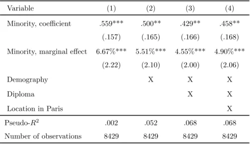
Table 1: Logit model of unemployment including a Minority dummy

Variable (1) (2) (3) (4)

Minority, coefficient .559*** .500** .429** .458** (.157) (.165) (.166) (.168) Minority, marginal effect 6.67%*** 5.51%*** 4.55%*** 4.90%***

(2.22) (2.10) (2.00) (2.06) Demography X X X Diploma X X Location in Paris X Pseudo-R2 _.002 _.052 _.068 _.068 Number of observations 8429 8429 8429 8429

Note: ***: significant at 1%; **: significant at 5%; *: significant at 10%.

school diploma, degree after two years in university, and degree with more than two years in university) and a dummy for living in the Paris urban unit. Results inTable 1 show that the coefficient on the Minority dummy does not vary much from a specification where only this dummy is introduced (column 1, coefficient: .559) to specifications obtained when adding groups of explanatory variables (columns 2 to 4, coefficient: .500, .429 and .458). This suggests that differences between the Minority and the Majority are not driven only by composition effects. The marginal effect of the Minority dummy is always sizable and around 5 percentage points. It has the same order of magnitude as the unexplained employment gap computed by Aeberhardt et al. (2010) for African second-generation immigrants which is 6.2 points.6

For workers occupying a job, we quantify the wage difference between the Majority and the Minority when the exact monthly wage is reported (and not a wage bracket). Keeping only reported wages which are strictly positive, we are left with 4, 139 observations (including 127 Minority members). When constructing the hourly wage from the monthly wage and the number of working hours when available, we are left with 4, 029 observations. The average wage for the Majority is 8.6 euros, and 31% lower for the Minority at 6.6 euros. When regressing the logarithm of wage on a dummy for Minority (column 1 in the top part ofTable 2), the estimated coefficient corresponds to a wage difference between the Majority and the Minority of 100 ∗ (exp(.208) − 1) = 23%. This

6_{Note that the two figures are not directly comparable as there can be some differences in the proportion of workers out of the labor} force between the Minority and Majority groups.

(10)

Table 2: Models of wage and commute differences Linear wage equation including a Minority dummy

Variable (1) (2) (3) (4) Minority, coefficient -.208*** -.198*** -.156*** -.194*** (.043) (.041) (.034) (.034) Demography X X X Diploma X X Location in Paris X R2 _.006 _.130 _.413 _.424 Number of observations 3850 3850 3850 3850

Linear commuting equation including a Minority dummy

Variable (1) (2) (3) (4) Minority, coefficient 9.911*** 10.904*** 11.631*** 4.516 (2.481) (2.524) (2.518) (2.449) Demography X X X Diploma X X Location in Paris X R2 _.002 _.004 _.011 _.082 Number of observations 6190 6190 6190 6190

figure is close to the 20% found byAeberhardt et al.(2010) who focus on African second-generation immigrants. The difference is lower in logarithm than in levels because the logarithm puts less weight on extreme values and the wage distribution is more dispersed for the Majority than for the Minority. The coefficient of −.208 does not vary much when adding the full set of controls (column 4) as it ends up at the value −.194.

Commuting time in the data corresponds to a return trip in minutes and is observed for 6, 511 of the 7, 500 workers with a job. We drop the 11 observations for which commuting time is larger than 4 hours and could correspond to coding mistakes. The average commuting time is 40.6 minutes for the Majority and nearly 10 minutes larger, at 50.5 minutes, for the Minority. The difference in average commuting time is partly explained by a fatter right tail of the distribution for the Minority than for the Majority, and the difference in median commuting

(11)

time is smaller at 5 minutes. Differences between the two groups may seem moderate but, in relative terms, they are rather large. Indeed, the average (median) commuting time is 24.1% (17.2%) larger for the Minority than for the Majority. We regress commuting time on a Minority dummy and controls. Results are reported in the bottom part ofTable 2 and show that the only factor really affecting the difference in commuting time between the Majority and the Minority is location. When introducing the dummy for living in the Paris urban unit, the difference drops to 4.5 minutes and is no longer significant as shown in column 4. However, it should be kept in mind that the Paris dummy captures location effects which should not be controlled for when calibrating the model as location effects should be captured by parameters related by spatial factors.

We investigate residential mobility using a variable giving the number of years spent in the current dwelling. Here, we consider a dummy for mobility taking the value one if households have spent three years or less in their dwelling and zero otherwise. The mobility rate for the Minority (30.9%) is larger than for the Majority (22.5%). We run a logit specification for mobility including a Minority dummy, and the results are reported in the top part ofTable 3. The difference in mobility between the Minority and the Majority grows larger when introducing demographic characteristics in the specification (columns 1 and 2). The marginal effect of the Minority dummy increases from 8.36% to 15.22%. It then remains stable when adding diplomas and location (columns 3 and 4).7 A likely reason for the higher mobility rate of the Minority is that Majority workers are more often owners and the mobility rate of owners is very low in France. In our sample, the ownership rate is 59.6% for the Majority and only 26.5% for the Minority. According to CGDD(2009), the mobility rate is only 3.8% for owners compared to 11.6% for public renters and 18.3% for private renters. Ideally, we would like to assess the effect of housing status three years before the survey date on the mobility difference between the Minority and the Majority but it is not available in the data. It should thus be kept in mind when interpreting the results of the model that mobility difference between the two groups partly captures effects related to ownership.

We also assess whether there are differences in mobility for specific reasons between the Majority and the Minority. For that purpose, we run a multinomial logit with three choices: no mobility, mobility for job-related reason (for one member of the household), mobility for another reason. Results reported in the bottom part of

Table 3show that the inclusion of demographic controls in the regression tends to increase the differences between

7_{Bouvard et al.}₍_2009b_{) report a lower mobility of African immigrants between urban unit size brackets than natives but a higher} proportion of moves within the same municipality. These results suggest that the larger mobility we find for the Minority group could be due to short-distance housing adjustments.

(12)

Table 3: Models of mobility including a Minority dummy Logit model of mobility including a Minority dummy

Variable (1) (2) (3) (4)

Minority, coefficient .430*** .904*** .940*** .938*** (.128) (.151) (.152) (.153) Minority, marginal effect 8.36%*** 15.22%*** 15.76%*** 15.73%***

(.027) (2.80) (2.81) (2.83) Demography X X X Diploma X X Location in Paris X Pseudo-R2 .001 .155 .161 .161 Number of observations 8392 8392 8392 8392

Multinomial logit model of mobility reasons including a Minority dummy

Variable (1) (2) (3) (4)

Mobility for job-related reason

Minority, coefficient .253 .760*** .824*** .839*** (.199) (.220) (.222) (.223) Minority, marginal effect 1.31% 3.81%* 4.27%** 4.48%**

(1.77) (2.09) (2.13) (2.17) Mobility for another reason

Minority, coefficient .528*** .959*** .978*** .963*** (.148) (.166) (.166) (.168) Minority, marginal effect 7.05%*** 11.19%*** 11.24%*** 10.93%***

(2.38) (2.64) (2.65) (2.65) Demography X X X Diploma X X Location in Paris X Pseudo-R2 _.001 _.124 _.131 _.131 Number of observations 8392 8392 8392 8392

(13)

the Majority and the Minority (columns 1 and 2). When all the observable characteristics are taken into account, the Minority group moves significantly more often than the Majority group both for job-related reasons and other reasons (column 4).

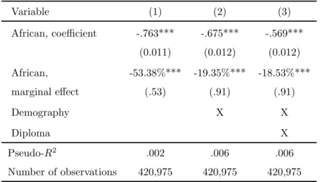
We also look at differences in unemployment duration and exit to jobs between French and African unemployed workers residing in the Paris region. Note that we do not have the data for all of France but the proportion of workers in the Minority group that are located in the Paris region is quite large according to the Time Use Suvey and stands at 43% (compared to 18% for the Majority group). Africans represent 12.3% of our sample. For unemployment spells beginning in the first semester of 1996, we know the exit when it occurs over the 1996-2003 period. This exit can be a job, a drop out of labour force or it can be unkown, in particular when there is an absence at control. Among unemployment spells for which exit is known, whereas 57.1% spells of French unemployed workers end with an exit to a job, the proportion is only 44.8% for African unemployed workers. The unemployment duration is 269 days for French unemployed workers exiting to a job but as large as 350 days for African ones. We run a Cox regression model for exit to a job to assess whether differences in unemployment duration between the French and Africans remain once observable characteristics have been taken into account. Exits other than finding a job (i.e. dropping out of the labor force, absence at a control, end of the panel) are treated as censored. In column (1) ofTable 4, only a dummy for being African is introduced and its effect is found to be significantly negative. The Africans have 53% less chances of finding a job than the French. Once all the explanatory variables have been introduced (column 3), the difference between the French and Africans is smaller but remains sizable as Africans still have 18% less of a chance of finding a job than the French.

Overall, our descriptive results suggest that there are some compositional effects but they tend to remain rather limited except for unemployment duration and commuting.

3 Model

We begin by considering a simple model where a geographical mobility decision interacts with a job acceptance decision. We follow the model inRupert and Wasmer(2012), where individuals search in the labor market and the housing market. They also face random housing shocks (leading them to relocate) and labor shocks. These shocks are assumed to be uncorrelated as described below. The goal of the model is to provide a decomposition of the sources of unemployment into a labor market component and a component due to spatial factors, for the Majority

(14)

Table 4: Cox duration model before exit to a job including a Minority dummy Variable (1) (2) (3) African, coefficient -.763*** -.675*** -.569*** (0.011) (0.012) (0.012) African, -53.38%*** -19.35%*** -18.53%*** marginal effect (.53) (.91) (.91) Demography X X Diploma X Pseudo-R2 _.002 _.006 _.006 Number of observations 420,975 420,975 420,975

and the Minority.

3.1 Preferences and Search for Locations

Time is continuous. Individuals face a rate of time preference equal to r. They can be employed or unemployed. When employed they live at some commute distance ρ from their job ; this distance varies as individuals randomly receive housing offers to which are associated commute distances drawn from a distribution GN(ρ), and they may

move to a new location allowing for shorter commute. The housing offers for the employed are assumed to be Poisson arrivals with parameter λH. Their dwelling is a bundle of services generating a flow of utility. For these

services, individuals pay a rent or a mortgage. We do not model the market for houses or locations and assume that moving to a new location is costless, but subject to frictions detailed below.8 _{We assume that the service}

flow from housing is equated across space and status so that we do not have to consider the cost of housing in our description.

The commuting time to one’s job becomes an important determinant of both job and location choice. Space is symmetric and isotropic, in the sense that the unemployed have the same chance of finding a job wherever their current residence. This assumption rules out specific effects of location on finding a job such as the help of a local

8_{For an alternative view where a spatialized housing market with endogenous rents is modelled, see the seminal works by}_Alonso (1974),Muth(1969) andMills(1972), as well as their sequels. In particular, extensions where both households and firms compete for land includeFujita and Ogawa(1982), andLucas and Rossi-Hansberg(2002).

(15)

network or the local diffusion of information on vacancies with wanted signs and local newspapers. It turns out that the distance to work, ρ, is a sufficient statistic determining job offer acceptance, housing offer acceptance and quits, the implication being there is no reason to move to a different location if unemployed.9

Agents may also receive a “family shock” due to changes in marital status, family size, schooling choices, neighborhood quality, and so on. Family shocks arrive according to a Poisson process with parameter δ. The shock changes the valuation of the current dwelling or location, necessitating a move. Upon the arrival of such a family shock, agents make one draw from the existing stock of housing vacancies. That is, while those employed who did not receive a family shock sample out of the new flow of vacancies, those who need to move due to that family shock only search through the existing stock.10 _{The type of shock thus indicates which distribution agents will be}

drawing from: either from the new vacancies coming on the market or from the existing stock of vacancies. This is in line with standard stock-flow models of the labor market.

As mentioned above, the distribution of new housing vacancies while employed is given as GN(ρ). The

distribu-tion of commuting distance for the unemployed receiving a job opportunity is given by another distribudistribu-tion F (ρ).11 The existing stock of housing vacancies is distributed as GS(ρ). Note that we will assume that GN stochastically

dominates GS, accounting for the well-known fact that new vacancies are generally of higher quality than the stock.

3.2 Labor Market

Individuals can be in one of two states: employed or unemployed. A match may become unprofitable, leading to a separation, which occurs exogenously with Poisson arrival rate s. While employed, income consists of an exogenous wage, w. We add taxes and benefits since these have been shown to affect unemployment rates across countries, as seen inMortensen and Pissarides(1999), for example. We assume a tax on labor denoted by t. The net wage reacts to taxes with a negative elasticity (a “crowding out” effect), so that an increase in taxes does not necessarily imply equivalent increases in labor costs. If taxes are t, the total labor cost is denoted by w(1 + εt) and the net wage of workers is w[1 − (1 − ε)t]. We set ε = 0.35 in line with elasticities from the literature and investigate the

9_{Rupert and Wasmer (2012) have a detailed discussion of this assumption.}

10_{The new flow of vacancies includes newly constructed dwellings and new vacancies of existing dwelling that are opportunities in} terms of commute distance.

11_{Note that having a constant arrival rate of job offers and a distribution of commuting distances associated with offers is equivalent} to receiving job offers with arrival rate depending on distance.

(16)

effect of alternative values in the robustness analysis.

Unemployed agents receive income b, where b can be thought of as unemployment insurance or the utility from not working. While unemployed, job offers arrive at Poisson rate p, indexed by a distance to work, ρ, drawn from the cumulative distribution function F (ρ).12 _{Job offers are not indexed by wage as we have imposed equal wages}

across all locations. Also, as is standard, we define θ as labor market tightness, or the vacancy to unemployment ratio.

Let E(ρ) be the value of employment for an individual residing at distance ρ from the job. Let U be the value of unemployment, which does not depend on distance, given the symmetry assumption made above. We can now express the problem in terms of the following Bellman equations:

(r + s)E(ρ) = w[1 − (1 − ε)t] − τ ρ + sU + λH

ˆ

max [0, (E(ρ0) − E(ρ))] dGN(ρ0) (1)

+δ ˆ

max[U − E(ρ), E(ρ00) − E(ρ)]dGS(ρ00)

(r + p)U = b + p ˆ

max[U, E(ρ0)]dF (ρ0), (2)

where τ is the per unit cost of commuting and ρ is the distance of the commute.13 _{Eq. 1}_{states that workers receive}

a utility flow w[1 − (1 − ε)t] − τ ρ; may lose their job and become unemployed – in which case they stay where they are; they may receive a housing offer from the distribution of new vacancies GN(ρ), which happens with intensity

λH, in which case they have the option of moving closer to their job. With Poisson intensity δ, they have to leave

their current location and draw a new distance ρ00which leads to an endogenous quit when the new location is too far away from the job.14 Eq. 2states that the unemployed enjoy b, and receive a job offer with Poisson intensity p, at a distance ρ0_{, from the distribution F (ρ). They have the option of rejecting the offer if the distance is too far.}

12_{Differences in the distribution of commute distances associated to job offers between the Majority and the Minority can exist} because employers may have chosen locations away from minorities or because minority workers may have been unable to locate close to employers because of housing market discrimination.

13_{It is tempting to reinterpret commuting as any non-pecuniary aspect of the job.} _{However, contrary to most job amenities,} commuting yields a monetary cost.

14_{Note that there is no on-the-job search. The only way for workers to change jobs is to quit their job to become unemployed and} then try to find a job elsewhere. Note that the quit rate here is endogenous. Adding job-to-job transitions would make the model more complicated and was not explored here. However, there are non-trivial transitions since family shocks affect employment-to-unemployment transitions.

(17)

3.3 Optimality and equilibrium conditions

Since all wages are assumed to be identical, the only relevant dimension of a job offer (or of a housing offer) is ρ, the distance (or time) of the commute. We denote by M_JE the rate at which employed workers move to get closer to their job. Job acceptance decisions when unemployed depend on the value of unemployment U relative to the value of a job at distance E(ρ). We denote by ρU _{the reservation distance above which job offers are rejected and}

below which they are accepted.

Job separation can occur in two ways: when there is an exogenous job destruction shock s, and when workers receive a family shock, δ, for which the new value of commuting distance is above ρU_{. Quits related to family}

shocks occur with Poisson intensity δ(1 − GS(ρu)). The overall separation rate is then

σ = s + δ(1 − GS(ρu)). (3)

On the firm’s side, jobs are created when the value of a vacancy is larger than its cost. Denote q(θ) as the Poisson hiring rate of workers, c the cost of a vacancy per unit of time, and y the value of productivity. Free entry of firms implies vacancies will be opened until firm profits are driven to zero.

Therefore, the four equations governing (ρU_{, θ, u, M}E J) are: ρU = w[1 − (1 − ε)t] − b τ + ˆ ρU 0 λHGN(ρ) + δGS(ρ) − θq(θ)F (ρ) r + s + λHGN(ρ) + δ dρ (4) F (ρU) = c q(θ) r + σ y − w(1 + ε)t (5) u = σ σ + θq(θ)F (ρU₎ (6) M_JE= (1 − u)λH ˆ ρU 0 GN(ρ)dΦ(ρ). (7)

The first equation comes from the equality of the value of unemployment and the value of employment; the second from the free-entry condition of firms; the third from the equality between the inflows into unemployment and the outflows from unemployment in steady-state; and the fourth from the rate of arrival of housing offers to the employed workers and the acceptance decision depending on the commuting distance involved. With this specification the model is quite parsimonious, since a single variable, ρ, determines job acceptance of the unemployed and the residential mobility rate.

(18)

Equation (4) establishes a negative link between labor market tightness, θ, and the reservation value of distance. The intuition is simple: in a fluid labor market (high θ and hence a high job finding rate θq(θ)) it is easier for a worker to wait for a better job offer. Hence workers accept offers only when the quality is higher (that is, when the commuting distance is lower). A more fluid housing market (higher λH) instead leads to higher acceptance rate

F (ρU) because workers can relocate more easily.

Equation (5) generates a positive link between θ and ρU since q0(θ) < 0. The intuition is also simple. The firm’s iso-profit curve at the entry stage depends negatively on both θ (as a higher θ implies more competition between firms and workers) and on ρU _{(as more of firm’s offers will be rejected because of distance). The zero-profit}

condition thus implies a positive link between θ and ρU_{. Note that this relation is independent of λ} H.

3.4 Decomposition of the unemployment rate gap

We seek to quantify the contribution of labor market and spatial factors in explaining the unemployment rate gap between distinct groups. Given the differences we have shown above, we will decompose the effects for Majority (subscript M), and Minority (subscript m). Note that the equilibrium unemployment rate u∗ depends on two sets of parameters: a labor block with job destruction s, labor productivity y, wage w, matching efficiency A and unemployment benefits b; and a spatial block with the arrival rate of housing offers λH, the parameter of their

distribution, α and the per unit cost of commute τ . In addition, firms face hiring costs c, and wages are taxed at rate t.

Denoting vectors of labor and spatial parameters respectively by L and S, and using the subscript M for the Majority and m for the Minority, we perform a Oaxaca decomposition of the unemployment gap between the Majority and the Minority in two different ways:

∆u = u∗(Lm, Sm) − u∗(LM, SM) = [u ∗_(L m, Sm) − u∗(Lm, SM)] | {z } spatial gap at Lm + [u∗(Lm, SM) − u∗(LM, SM)] | {z } labor gap at SM = [u ∗_(L m, Sm) − u∗(LM, Sm)] | {z } labor gap at Sm + [u∗(LM, Sm) − u∗(LM, SM)] | {z } spatial gap at LM .

(19)

4 Numerical exercise

4.1 Calibration strategy

The strategy is to treat each group (the Majority and the Minority) separately, that is, we calibrate the model on two independent segments of the labor market. The calibration will match job-related mobility and the unemployment rate. Without loss of generality we normalize average productivity and labor market tightness to 1.

4.2 Parameters

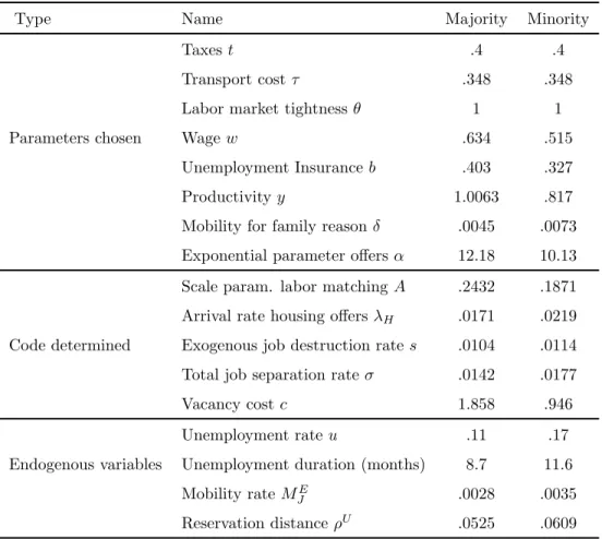
In our benchmark case, we consider that some parameters will be different and some common for the two groups, consistent with the data. We first describe those parameters that we allow to differ between groups. The parameters are summarized inTable 6.

In the benchmark we allow for differences in Majority and Minority wages and then exogenously fix the wage for each group. The wage difference target is based onTable 2, column 1. In that column, we find a 20.8% log-wage gap between the Majority and the Minority. Given the proportion of each group in the total population, this imposes that Majority wage is .6% above the population average wage (itself equal to .63 with a labor productivity equal to 1) and the Minority wage is therefore 20.2% below the average. In France, in the range of hourly wages of the two groups (on average between 6.55 euros for the Minority and 8.62 for the Majority), unemployment benefits are proportional to wages according to the rules of unemployment compensation. Accordingly, we impose the same unemployment benefits differences, that is b = .403 for the Majority and b = .327 for the Minority. Productivities of the two subgoups corresponding to wages are y = 1.0063 for the Majority and y = .817 for the Minority.

In the model, we have three distributions of commute distances that are related to job offers, new housing vacancies, and the stock of housing vacancies. We assume that these distributions can be represented by exponential functions with parameter α: F (ρ) = GN(ρ) = 1 − e−αρ and GS(ρ) = 1 − e−(α/3)ρ. Here, 1/α is both the average

commuting distance and the standard error of commuting distances for new vacancies and job offers. The average distance for the stock of vacancies is three times higher than the average distance for new vacancies.15 The parameter α is computed by fitting an exponential distribution to the distribution of commute times of employed

15_{Rupert and Wasmer (2012) show that the quantitative results are not sensitive to the exact distribution G}

S. This is because family shocks do not have a large impact on labor market margins.

(20)

Table 5: Commute time as a fraction of standard daily working time (7.8 hours) All Majority Minority Relative difference (%) Mean .089 .087 .108 24.1%

Median .064 .064 .075 17.2%

Figure 1: Cumulative of commuting time for the Minority and the Majority

0 .2 .4 .6 .8 1 0 .1 .2 .3 .4 .5 0 .2 .4 .6 .8 1 0 .1 .2 .3 .4 .5 Minority Majority

In blue: empirical cumulative; in red: cumulative of an exponential law with parameter α = 10.13 for the Minority and α = 12.18 for the Majority.

workers.16 _{Ordinary least squares were applied to a specification derived from the equality −ln [1 − F (ρ)] = αρ}

for exponential laws, where the cumulative of commute times F has been replaced by its empirical counterpart and a sampling error has been added on the right-hand side. Commute times are for return trips and are expressed as a fraction of standard daily working time (7.8 hours). Table 5 reports some descriptive statistics on these standardized commute times. We find empirically that α = 10.13 for the Minority and α = 12.18 for the Majority. Figure1represents the empirical cumulative and the fitted exponential cumulative for each of the two groups.

Targets corresponding to mobility for family reasons and mobility for job related reasons (δ and M_JE, respec-tively) are calculated from the observed mobility rates within the last three years for the Majority and the Minority.

16_{Note that we make an approximation as parameter α is estimated from the equilibrium distribution of commute distances and not} from the distribution of job offers to unemployed workers (whether they are accepted or not). We verified after the calibration of the model that the equilibrium distribution of commute distances implied by equation (11) when using the calibration parameters is not too different from the distribution of job offers to unemployed workers F (ρ) once it has been truncated in ρU_{, which we denote F}

t(ρ). We computed a Pseudo-R2 _{as 1 −}P60

k=1[Φ(ρk) − Ft(ρk)]2/P60k=1Φ(ρk)2where ρk, k = 1..., 60 are values of ρ uniformely distributed over the range [0, ρu]. This Pseudo-R2 takes the value .99 both for the Minority and the Majority.

(21)

Table 6: Parameters of the model for the Majority and the Minority, France

Type Name Majority Minority

Taxes t .4 .4

Transport cost τ .348 .348 Labor market tightness θ 1 1 Parameters chosen Wage w .634 .515

Unemployment Insurance b .403 .327 Productivity y 1.0063 .817 Mobility for family reason δ .0045 .0073 Exponential parameter offers α 12.18 10.13 Scale param. labor matching A .2432 .1871 Arrival rate housing offers λH .0171 .0219

Code determined Exogenous job destruction rate s .0104 .0114 Total job separation rate σ .0142 .0177 Vacancy cost c 1.858 .946 Unemployment rate u .11 .17 Endogenous variables Unemployment duration (months) 8.7 11.6

Mobility rate ME

J .0028 .0035

(22)

For an exponential law, the probability of not moving for a family-related reason before a duration T0 is given by

P (T > T0) = e−δT0. As moving within the last three years is defined as having a housing tenure being 0, 1 or 2

years, there is some discretion in the value for T0 and we fix T0 = 30 months (ie. 2.5 years). The mobility rate

for family-related reasons is 12.75% for the Majority and 19.73% for the Minority. It corresponds to a monthly parameter δ given by −ln (1 − .1275) /30 = .0045 for the Majority and −ln (1 − .1973) /30 = .0073 for the Minority. As regards to mobility for job-related reasons, we apply the same formulas. There are however two alternatives for the calculation of mobility rates for job-related reasons: in the first one, we define job-related reasons for any member of the household, and in the second one, we only consider job-related reasons for the surveyed worker (restricting the computation to the household head and possibly his partner). Under the first alternative, the mobility rates of the Majority and the Minority are respectively 8.10% and 9.87%. The corresponding mobility rates ME

J are respectively −ln (1 − .0810) /30 = .0028 and −ln (1 − .0987) /30 = .0035. We choose the first

alternative, and use these values in the calibration.17

The rate of exit from unemployment is given by p(θ)F (ρU) with p(θ) = Aθ0.5 where θ is the labor market tightness and A is a scale parameter. Setting θ = 1 gives A = .2432 for Majority workers and A = .1871 for Minority workers. Together with the free-entry condition (Eq. 5), this fixes a value for recruiting costs c after normalizing y for the two groups.

We also set some parameters common to the two groups. Labor tax rate is fixed at its value in France which is t = .4, seeRupert and Wasmer(2012). We also fix the transport cost τ to a common value in the following way. Each hour of commute time has a utility cost supposed to be half the hourly wage of workers in line withSmall and

Verhoef(2006). The median commuter spends 6.4% of the standard daily working time (7.8 hours) to commute as

shown inTable 5. Hence, the total median cost for the median commuter should be .064/2 expressed as a fraction of the wage, that is .064/2∗(w/y).18 The total median cost is also calculated from the distribution of wage offers for the whole labour force. The median commuting distance is computed as ρm = ln(2)/α` with α` = 11.97 the

parameter of an exponential law fitting the distribution of commute times for the whole labour force. The total

17_{Under the second alternative, the mobility rates of the Majority and the Minority are respectively 5.72% and 6.70%. The} corre-sponding parameters ME

J are respectively −ln (1 − .0572) /30 = .0020 and −ln (1 − .0670) /30 = .0023. 18_{Note that the ratio w/y is the same for the Minority and the Majority and equal to .63 by construction.}

(23)

cost incurred by the median commuter is therefore given by .064/2 ∗ (w/y) = τ ρm_{or equivalently:}

τ = .064/2 ∗ (w/y) ln2/α`

= .3481. (8)

The program finds the parameters of the model given target unemployment rates of 11% for the Majority and 17% for the Minority, and target exit rates from unemployment to a job of p(θ)F (ρU_{) = 1/8.7 and 1/11.6}

monthly for those two groups, thus fixing the job separation rate σ given that the unemployment rate verifies u = σ/(σ + p(θ)). In addition, the program finds the housing arrival rate λH that is consistent with the target for

mobility, given the reservation distance ρU, obtained from (Eq. 4).

4.3 Findings

Findings for the benchmark case are given inTable 6. Interestingly, whereas the arrival rate of housing offers, λH,

is higher for the Minority than the Majority, the parameter of the commuting distribution α is smaller. This means that Minority workers have more housing offers, but their housing offers are associated with longer commuting distances. A possible interpretation is that Minority workers get more housing offers because they are more often renters than Majority workers and put more efforts in looking for a dwelling to make housing adjustments, in particular in terms of location.19 _{However, because of their residential location and the spatial distribution of jobs,}

they get housing offers associated on average with larger commuting distances than Majority workers.

We also find that the reservation distance ρU is larger for the Minority suggesting that Minority workers are less choosy for commuting distances associated with housing offers.

Turning to labor market parameters, the scale parameter of the matching function A is smaller for the Minority than for the Majority. This result suggests that matching is less efficient for the Minority group possibly because of composition effects or discrimination. Jobs occupied by Minority workers are also more likely to be destroyed. In fact, the difference in the separation rate, σ, between the Minority and the Majority is even larger than the difference in job destruction rate s. This means that separations due to family shocks are more likely. As shown by

Eq. 3, this occurs both because family shocks δ are more frequent for the Minority and because Minority workers

are less choosy when receiving the housing offer related to the family shock. Finally, the vacancy cost c is lower for Minority workers, possibly because jobs that Minority workers occupy are of lower quality and their vacancy is less costly.

(24)

We evaluate the effect on the unemployment rate u, reservation distance ρU_{, and mobility rate for job-related}

reasons ME

J by changing sequentially the parameters from their value for the Minority to their value for the Majority.

We focus on the unemployment rate which is our main variable of interest. We perform our decompositions of the difference in the unemployment rate between the Minority and the Majority as described in Section 3.4. These decompositions allow us to assess the respective importance of differences in labor market factors and differences in spatial factors. Among the labor market parameters, the only parameter which is supposed to be the same for the two groups is the matching efficiency θ. The Minority and the Majority differ for the other parameters which are the labor productivity y, wage w, unemployment benefits b, job destruction rate s, matching efficiency A, job separation rate σ and vacancy cost c. Among spatial parameters, the commuting cost τ is supposed to be the same for the two groups, such that the Minority and the Majority differ only in their arrival rate of housing offers λH

and the parameter of the commuting distribution α.

Results when changing the parameters from their value for the Majority to their value for the Minority are reported in Panel A of Table 7 and show that commuting distances play a significant role. When changing the parameter of the commuting distribution α, the Minority unemployment rate decreases from 17.0% to 15.04%: thus, 1.96 percentage points of the six percentage points difference, or 32.7% of the unemployment gap is accounted for by less favorable housing offers in terms of commuting distance. Additionnally changing the arrival rate of housing offers λH to the (lower) value of the Majority compensate to some extent the differences in housing offers since it

makes the unemployment rate raise again to 15.47%. Overall, the two parameters account for 17 − 15.47 = 1.53 points of the 6 points unemployment gap or 25.5% of the difference. Some labour parameters play a more important role. Indeed, changing the scale parameter of the matching function A affects the Minority unemployment rate significantly as it decreases to 12.67%. A change in the job destruction rate s also significantly affects the Minority unemployment rate as it decreases to 12.03%. Additionnally changing the wage, unemployment benefits and productivity decreases a lot the unemployment rate which is then 9.70%. The last column is then reached when the last parameters differing across groups (the vacancy posting costs and the family parameter δ) are equal to that of the Majority group. Since this raises the unemployment rate from 9.70% back to 11%.

Some comparative statics are also conducted changing sequentially the parameters from their value for Majority to their value for the Minority and results are reported in Panel B ofTable 7. Results confirm our previous findings, though with slightly different values. Applying the parameter of the commuting distribution α of the Minority to

(25)

the Majority raises unemployment from 11% to 12.42%, or 1.42 points of the unemployment gap, that is 23.7% of the gap. Raising the value of the arrival rate of offers to the value of the Minority decreases the unemployment rate to 12.04%. Here, the two parameters α and λh account for 1.04 points of the total unemployment gap, that

is 17.3%.

According to these comparative statics, there are differences in the commuting distances associated to housing offers which explain a significant part of the unemployment rate gap. The arrival rate of housing offers varies across groups to compensate for the differences in housing offers. That is, the Minority may be getting more housing offers but their offers would be associated to longer commuting distances. This may be due to search in different housing market segments or different search intensity with search intensity being endogenous; however, we leave this for future research. Bouvard et al.(2009b) would rationalize our finding with the progressive sectoral shift in France from industrial jobs close to dwellings of immigrants to service jobs in cities that immigrants cannot easily access.

Overall, although labor factors play a major role, spatial factors play a significant role in this benchmark specification, between 17% and 25.5% of the unemployment gap, depending on the decomposition exercise which is considered. The next Section is devoted to an assessment of the robustness of this result.

5 Alternative specifications

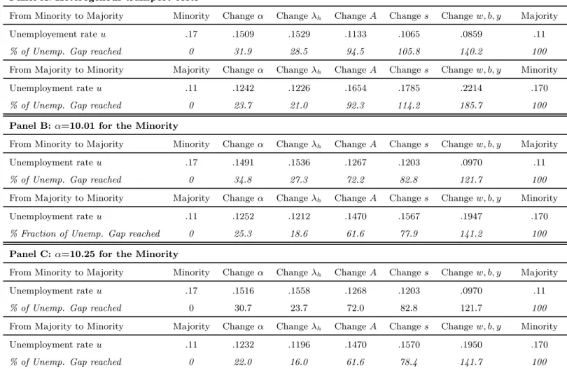
So far, we have considered that commuting costs are the same across groups. In this section we relax this strong assumption and do robustness checks on the values of parameters α. We finally assess whether results are stable when we change the wage gap between the Minority and the Majority, as well as the elasticity of wages with respect to taxes.

The Minority and the Majority may not have access to the same transportation modes, and this can generate a difference in transport costs between the two groups. As a consequence, we now consider the case where the Minority and the Majority have different transport costs evaluating formula (8) with the value of α specific to each group, which gives: τ = .3542 for the Majority and τ = .2946 for the Minority. All other parameters are the same as in the previous Section. This changes the parameter estimates and leads to the decompositions given in Panel

A ofTable 8. The conclusions we drew fromTable 6remain the same.

(26)

Table 7: Comparative Statics from Minority parameters to Majority parameters and vice-versa, France*

Panel A: From Minority to Majority

Minority Change α Change λh Change A Change s Change b, w, y Majority

Commute distribution parameter α 10.13 12.18 12.18 12.18 12.18 12.18 12.18

Arrival rate housing offers λH .0219 .0219 .0171 .0171 .0171 .0171 .0171

Scale parameter matching A .1871 .1871 .1871 .2432 .2432 .2432 .2432

Job destruction rate s .0114 .0114 .0114 .0114 .0104 .0104 .0104

Unemployment rate u .1700 .1504 .1547 .1267 .1203 .0970 .1100

% of Unemp. Gap reached 0 32.7 25.5 72.1 82.8 121.7 100

Reservation distance ρU _.0609 _.0558 _.0546 _.0452 _.0438 _.0447 _.0525

Mobility rate ME

J .0035 .0037 .0029 .0026 .0025 .0025 .0028

Panel B: From Majority to Minority

Majority Change α Change λh Change A Change s Change b, w, y Minority

Commute distribution parameter α 12.18 10.13 10.13 10.13 10.13 10.13 10.13

Arrival rate housing offers λH .0171 .0171 .0219 .0219 .0219 .0219 .0219

Scale parameter matching A .2432 .2432 .2432 .1871 .1871 .1871 .1871

Job destruction rate s .0104 .0104 .0104 .0104 .0114 .0114 .0114

Reservation distance ρU _.0525 _.0577 _.0591 _.0719 _.0745 _.0717 _.0609

Mobility rate ME

J .0028 .0026 .0033 .0038 .0039 .0038 .0035

*Note: α is the parameter of the exponential distribution of commute offers; λHis the arrival rate of housing offers;

(27)

affecting the accuracy of the estimator as can be seen from its standard deviation. Indeed, we find for the Minority α = 10.13(.12) whereas we have for the Majority α = 12.18(.016). Therefore, we re-estimate the model to assess the robustness of our results when varying the value of α for the Minority and using either α = 10.13 − .12 = 10.01 or α = 10.13 + .12 = 10.25. The parameter for the Majority is kept the same, the decompositions are in Panel B and C ofTable 8; again, our main conclusions remain unaltered.

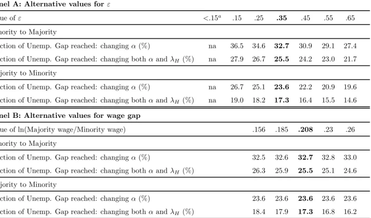
Next, we vary the elasticity of the response of gross and net wages: recall that we assumed the labor cost increase caused by tax to be εt and the net wage decrease to be (1 − ε)t. We now only report the fraction of the unemployment gap that can be explained by a change in α and a cumulated change in both α and λh for both

decomposition exercises. The benchmark value of ε is .35. Below .15 the code did not converge, because we reached a corner solution where all the wage offers to the Minority are accepted. However, over the range .15 to .65, the results of the decomposition exercise are very stable as shown in Panel A ofTable 9, and if anything, the role of spatial factors in the determination of unemployment increases as ε decreases.

The next table investigates the effect of alternative values of the wage gap between the Majority and the Minority, also reflected in unemployment benefits and productivity. Our benchmark value is derived from the gross log-wage gap, 20.8%, which is given by Table 2, column (1). We now vary this gap from the lowest value in the table, 15.6%, which is reached in column (3) when controlling for demographic factors and diplomas, up to 26%. Comparative static results reported in Panel B ofTable 9are very similar to those obtained in the benchmark case regarding the fraction of the unemployment rate gap explained with the differences in the commuting distribution parameter and in the arrival rate in housing offers between the Minority and the Majority.

6 Comparison with the US

The calibration exercise is replicated for the US to study the unemployment rate difference between Blacks and Whites, with the values of the unemployment rate in 2011, the median unemployment duration in 2011 and the 2010-2011 Census mobility rates. Commute time data comes from the US Census American Community Survey.20

Note that while we use the terms Majority and Minority for the French data our analysis for the US covers only Whites and Blacks. A Mincerian regression analogous to those in Table 2 delivers a hourly wage premium to white

20_{Data are available as frequencies in commute time brackets. Therefore, we computed the commute time parameter α for Blacks} and for Whites using moment conditions based on the cumulative of the exponential law rather than linear regressions.

(28)

Table 8: Comparative Statics using alternative values of transport cost parameter and commute time parameter for the Minority, France

Panel A: Heterogenous transport costs

From Minority to Majority Minority Change α Change λh Change A Change s Change w, b, y Majority

Unemployement rate u .17 .1509 .1529 .1133 .1065 .0859 .11

From Majority to Minority Majority Change α Change λh Change A Change s Change w, b, y Minority

Panel B: α=10.01 for the Minority

% Fraction of Unemp. Gap reached 0 25.3 18.6 61.6 77.9 141.2 100

Panel C: α=10.25 for the Minority

Note: α is the parameter of the exponential distribution of commute offers; λH is the arrival rate of housing offers;

(29)

Table 9: Comparative Statics using alternative values for ε and wage gap, France Panel A: Alternative values for ε

Value of ε <.15a _.15 _.25 _.35 _.45 _.55 _.65

Minority to Majority

Fraction of Unemp. Gap reached: changing α (%) na 36.5 34.6 32.7 30.9 29.1 27.4 Fraction of Unemp. Gap reached: changing both α and λH (%) na 27.9 26.7 25.5 24.2 23.0 21.7

Majority to Minority

Fraction of Unemp. Gap reached: changing α (%) na 26.7 25.1 23.6 22.2 20.9 19.6 Fraction of Unemp. Gap reached: changing both α and λH (%) na 19.0 18.2 17.3 16.4 15.5 14.6

Panel B: Alternative values for wage gap

Value of ln(Majority wage/Minority wage) .156 .185 .208 .23 .26 Minority to Majority

Fraction of Unemp. Gap reached: changing α (%) 32.5 32.6 32.7 32.8 33.0 Fraction of Unemp. Gap reached: changing both α and λH (%) 26.3 25.9 25.5 25.1 24.6

Fraction of Unemp. Gap reached: changing α (%) 23.6 23.6 23.6 23.6 23.6 Fraction of Unemp. Gap reached: changing both α and λH (%) 18.4 17.9 17.3 16.8 16.2

Note: Columns corresponding to the benchmark are in bold.a_{: Reach a corner solution with ρ} U= 0.

(30)

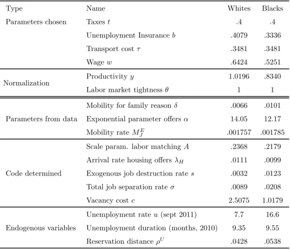
Table 10: Parameters for Whites and Blacks (U.S.) with the same benefits and tax system as in Europe

Type Name Whites Blacks

Parameters chosen Taxes t .4 .4 Unemployment Insurance b .4079 .3336 Transport cost τ .3481 .3481

Wage w .6424 .5251

Normalization Productivity y 1.0196 .8340 Labor market tightness θ 1 1 Mobility for family reason δ .0066 .0101 Parameters from data Exponential parameter offers α 14.05 12.17 Mobility rate M_JE .001757 .001785 Scale param. labor matching A .2368 .2179 Arrival rate housing offers λH .0111 .0099

Code determined Exogenous job destruction rate s .0032 .0123 Total job separation rate σ .0089 .0208 Vacancy cost c 2.5075 1.0179 Unemployment rate u (sept 2011) 7.7 16.6 Endogenous variables Unemployment duration (months, 2010) 9.35 9.55 Reservation distance ρU .0428 .0538

workers as compared to black workers that is close to that of France, that is 20.1% in the US. We will use this value in the US calibration. As a first pass, we also use the same tax rate, unemployment insurance and transport costs as in France, to focus on the role of different unemployment and mobility targets and progressively relax these values.

The calibration parameters obtained present some similarities with those of France: the search cost, for in-stance, is higher for Majority workers than for Minority workers. Here however, the arrival rate of housing offers λh turns out to be lower: therefore, the two parameters reinforce each other in generating racial differences in

un-employment rates. The total racial difference to be explained in the US is 16.6%-7.7%= 8.9%. However, the share explained by the spatial parameters is actually smaller than in France, since, depending on the decomposition, these parameters explain either (8.60-7.7)/8.9=10.1% in the first decomposition, or (16.6-15.05)/8.9=17.5% in the second decomposition.

(31)

Table 11: Comparative Statics from Whites to Blacks and vice-versa, US

From White to Black parameters Whites Change α Change λh Change A Change s Change w, b, y Blacks

Fraction of Unemp. Gap reached (%) 0 9.0 10.1 16.2 106.2 149.9 100

From Black to White parameters Blacks Change α Change λh Change A Change s Change w, b, y Whites

Fraction of Unemp. Gap reached (%) 0 16.3 17.5 28.1 88.5 107.1 100

Next, we change the values of unemployment benefits and taxes. For unemployment benefits, we choose a lower range, from b = .3 to .25 instead of b = .4. For taxes, we choose a range of .25 to .4. We obtain the results inTable 12

which roughly confirms the message of the previous table: the share of the ethnic unemployment gap explained by spatial factors remains limited, in a range of 8% to 17.6% of the total difference across groups. Convergence problems arise with lower values of taxes and benefits, since the unemployment rate and unemployment duration to be matched by the model are relatively large due to the specific period retained which is year 2011.

Our decomposition exercises show that there are differences between France and the US that are not related to differences in institutional parameters. Whereas, in the two countries, the unemployment rate gap between the Majority and the Minority is explained to some extent by ethnic differences in the distribution of commute distances, mobility plays a different role. In France, higher commute distances for the Minority are mitigated by a mobility rate which is higher than that of the Majority. By contrast, in the US, higher commute distances for the Minority are reinforced by a lower mobility rate. In the two countries, though, calibrations imply that ethnic differences in commute offers explain about two percentage points of the ethnic unemployment rate gap. In addition, in the US, blacks have a separation rate which is four times higher than that of whites, and differences in the labor market parameters between the two groups imply a larger ethnic unemployment rate gap than in France. This leads to a lower fraction of the unemployment gap explained by spatial parameters in the US, and a larger contribution of the labor parameters.

7 Concluding Comments

To better understand the relationship of housing and labor markets we construct an integrated model of unem-ployment and mobility that can be calibrated to assess the extent to which the unemunem-ployment rate is related to

(32)

Table 12: Comparative Statics from Minority parameters to Majority parameters, alternative values of benefits and taxes, US

Different values of benefits b Different values of taxes .25a _.30 _.35 _.40 _.40 _.35 _.30 _.25

Fraction of the gap reached with a change in α (%) na 7.7 8.4 9.0 9.0 8.7 8.5 8.2 Fraction of the gap reached: change α and λH (%) na 8.4 9.2 10.4 10.4 9.7 9.4 9.0

Fraction of the gap reached with a change in α (%) na 13.0 14.6 16.1 16.1 15.6 14.9 14.2 Fraction of the gap reached: change α and λH (%) na 13.6 15.4 17.6 17.6 16.6 15.8 15.0

Note: Columns corresponding to the benchmark are in bold.a_{: Reach a corner solution with ρ} U= 0.

labor market factors and spatial factors.

Based on calibrations of the model, we develop a decomposition of the unemployment rate gap between the Majority and a Minority, both in France and the US. We find that the effect of differences between groups in spatial factors is significant: it generates an unemployment rate difference of about 1 to 1.5 percentage points both in France and the US. Since the gap itself is 6 percentage points in France and 8.9 percentage points in the US, differences in spatial factors represent 17% to 25% of the unemployment rate gap in France, and 10% to 17.5% of the gap in the US.

The significant impact of spatial factors in explaining the unemployment rate gap between the Majority and the Minority in France is due to differences in commuting distances related to housing offers, that is, access to housing offers close enough to the locations of jobs, or reciprocally, access to job offers close enough to housing. This may be related to spatial mismatch as, in France, it is well known that areas located far from jobs, often referred to as “quartiers sensibles”, are prone to major difficulties such as high unemployment, lack of social integration and crime.

Differences in these commuting distances accounts for a large fraction of the unemployment rate gap. The Minority receives more frequent offers, such that additionally taking into account differences in the arrival rate of housing offers reduces the contribution of spatial factors to explaining the unemployment rate gap. Overall, we still conclude that labor market factors remain the main explanation for the higher unemployment rate of Africans.

(33)

housing markets interact in complex ways; indeed, it is not always easy to find an appropriate natural experiment to properly decompose the respective role of each market on unemployment. For instance, our approach could be used to better understand the unemployment of secondary wage earners, as well as the effect of transportation policies and taxation of gasoline on unemployment.