Publisher’s version / Version de l'éditeur:
Questions? Contact the NRC Publications Archive team at
[email protected]. If you wish to email the authors directly, please see the first page of the publication for their contact information.
https://publications-cnrc.canada.ca/fra/droits
L’accès à ce site Web et l’utilisation de son contenu sont assujettis aux conditions présentées dans le site LISEZ CES CONDITIONS ATTENTIVEMENT AVANT D’UTILISER CE SITE WEB.
Internal Report (National Research Council of Canada. Institute for Research in
Construction), 2002-05-01
READ THESE TERMS AND CONDITIONS CAREFULLY BEFORE USING THIS WEBSITE. https://nrc-publications.canada.ca/eng/copyright
NRC Publications Archive Record / Notice des Archives des publications du CNRC :
https://nrc-publications.canada.ca/eng/view/object/?id=6d7ecbac-65c7-440b-a38a-e8bd59f2e39f https://publications-cnrc.canada.ca/fra/voir/objet/?id=6d7ecbac-65c7-440b-a38a-e8bd59f2e39f
Archives des publications du CNRC
For the publisher’s version, please access the DOI link below./ Pour consulter la version de l’éditeur, utilisez le lien DOI ci-dessous.
https://doi.org/10.4224/20378987
Access and use of this website and the material on it are subject to the Terms and Conditions set forth at
UMAR theory & user manual: version 1.0
Martin-Pérez, B.; Nofal, M.
www.nrc.ca/irc/ircpubs
IR-852
Institute for Institut de
Research recherche
In Construction en construction
UMAR
Theory & User Manual
Version 1.0
B. Martín-Pérez and M. Nofal
Internal Report No. 852
1 INTRODUCTION...1
2 PROGRAM STRUCTURE...2
3 ELEMENT LIBRARY...4
3.1 SPACE TRUSS ELEMENT...4
3.2 SHEAR CONNECTOR ELEMENT...6
3.3 REFINED QUADRILATERAL PLANE ELEMENT (RQD4) ...8
3.4 PLATE BENDING ELEMENTS...12
3.4.1 Quadrilateral bending element (QBE) ... 12
3.4.2 Improved discrete Kirchhoff quadrilateral (IDKQ)... 13
3.5 QUADRILATERAL FACET SHELL ELEMENT (QFSE) ...23
3.6 SOLID ISOPARAMETRIC ELEMENT...26
3.6.1 Layered solid isoparametric element ... 29
4 MATERIAL LIBRARY...31
4.1 THEORY OF ELASTICITY...31
4.1.1 Linear elastic model ... 31
4.1.2 Orthotropic hypoelastic model ... 36
4.1.3 Resilient modulus models... 42
4.2 THEORY OF PLASTICITY...44
4.2.1 Yield criteria ... 44
4.2.2 Hardening laws ... 47
4.2.3 Rate-independent plastic model ... 50
4.2.4 Isotropic visco-plastic model ... 51
4.3 THEORY OF CONTINUUM DAMAGE MECHANICS...54
4.3.1 Crack compliance... 56
4.3.2 Crack evolution criteria ... 63
5 STRUCTURAL ANALYSIS...73 5.1 BOUNDARY CONDITIONS...74 5.2 SOLUTION PROCEDURE...74 5.2.1 Material non-linearity... 74 5.3 CONVERGENCE CRITERIA...76 6 CONSTRUCTION ANALYSIS...78 6.1 REMOVAL ANALYSIS...78 6.2 RESTORATION ANALYSIS...78 7 TRANSIENT ANALYSIS...79 7.1 GOVERNING EQUATION...79 7.2 BOUNDARY CONDITIONS...79
7.3 FINITE ELEMENT FORMULATION...80
7.4 TRANSIENT ELEMENTS...82
7.5 NUMERICAL SOLUTION...82
8 TYPES OF SOLVERS ...83
8.1 LU DECOMPOSITION METHOD...83
8.3 GAUSS-SEIDEL METHOD...84
8.4 DOMAIN DECOMPOSITION METHOD...85
8.5 BICONJUGATE GRADIENT METHOD...87
8.5.1 Convergence criteria... 88
9 REFERENCES...90
APPENDIX A: USING THE PROGRAM ...94
A.1 ENTERING REQUIRED INPUT...94
A.2 READING PROGRAM OUTPUT... 105
TABLE OF FIGURES
Figure 2-1: Modular nature of program UMAR. ... 2
Figure 3-1: Space truss element. ... 5
Figure 3-2: Shear connector element... 6
Figure 3-3: Load-slip relationship for the shear connector [44]. ... 7
Figure 3-4: Elements QUAD8 and RQD4... 9
Figure 3-5: Normal displacement un to side 1-2 due to w1 = 1. ... 10
Figure 3-6: Plate bending elements QBE and IDKQ. ... 13
Figure 3-7: Transformation of element QUAD9 into element IDKQ. ... 14
Figure 3-8: Co-ordinate transformation along of the side of a QUAD9 element... 16
Figure 3-9: The facet shell element QFSE. ... 23
Figure 3-10: Layered shell element... 25
Figure 3-11: Hexahedral elements of the “serendipity” family implemented in UMAR. ... 26
Figure 3-12: Eight-to-twenty nodes solid isoparametric element. ... 27
Figure 4-1: Uniaxial stress-strain curve for compressive and tensile loading. ... 38
Figure 4-2: (a) Crack formation in principal tension direction; (b) Tensile uniaxial stress-strain curve... 40
Figure 4-3: Triaxial compressive strength envelope. ... 41
Figure 4-4: Triaxial tensile strength envelope. ... 42
Figure 4-5: Rheological analogue of elasto-visco-plastic model. ... 52
Figure 4-6: Typical section subjected to general state of stresses... 58
Figure 4-7: Flowchart to implement micro-mechanical damage-based model [27]... 72
Figure 5-1: Algorithm implemented in UMAR for non-linear analysis. ... 76
Figure 6-1: Removal forces (adapted from [38]). ... 78
TABLE OF TABLES
Table 4-1: Constants defining isotropic yield surfaces implemented in UMAR. ... 49
Table 7-1: Correspondence between Eq. 7.1 and the governing differential equations. ... 79
Table 7-2: Correspondence between Eq. 7.2 and the imposed boundary conditions. ... 80
Table A-1: Heading information. ... 95
Table A-2: Control data (refer to Table A-3.)... 95
Table A-3: Input indicators for control data. ... 96
Table A-4: User output options... 96
Table A-5: Nodal point data. ... 97
Table A-6: Material data. ... 97
Table A-7: Constitutive models implemented in program UMAR. ... 99
Table A-8: Yield criteria and hardening functions implemented in program UMAR... 99
Table A-9: Equivalent yield stress. ... 99
Table A-10: Layering systems data... 100
Table A-11: Cross-section data (refer to Table A-12.)... 100
Table A-12: Input indicators for cross sections data. ... 101
Table A-13: Element data... 101
Table A-14: Line commands for different element types... 102
Table A-15: Deformation boundary conditions data (if stress analysis required.)... 102
Table A-16: Analysis data for field problems (if thermal or/and hygroscopic or/and chloride analysis required.)... 102
Table A-17: Numerical data. ... 103
Table A-18: Load data for each time step if stress, removal or restoration analysis required. .... 103
Table A-19: Input indicators for load data. ... 103
1 Introduction
Program UMAR, which stands for Unified Method of Analysis for Rehabilitation, is a general-purpose finite element program for rehabilitation analysis and design of various structural and building components. UMAR solves for the static response of linear and non-linear two- and three-dimensional structural systems under the action of mechanical loads. The computer program can include time-dependent phenomena such as creep, shrinkage and cyclic loading. UMAR also offers transient analysis capabilities for parabolic initial-value problems in fluid mechanics, and it can couple this type of analysis with that due to mechanical loads. Some features which are available in the program include:
! Multi-field/physics analysis capabilities to couple heat-mass transfer problems with stress problems;
! Element options to model addition or removal of elements (material) in the physical system to simulate construction/rehabilitation processes;
! Six basic elements for structural analysis: a space truss element, a shear connector element, a quadrilateral membrane element, a quadrilateral plate-bending element, a quadrilateral shell element, and a layered-solid element. All the quadrilateral elements can be layered in the out-of-plane direction. The membrane and solid elements can also be used for transient analysis; ! Prescribed nodal displacements and/or surface traction options for structural analysis; ! Prescribed nodal values and/or surface flux options for transient analysis;
! Prescribed arbitrary load-time functions (both mechanical and environmental);
! Comprehensive library of material models: isotropic linear-elastic, orthotropic linear-elastic, transversely-isotropic linear-elastic, orthotropic hypo-elastic, elasto-(plastic)-damage, and a family of multi-yield elasto(-visco)-plastic;
! Several symmetric and non-symmetric matrix equation solvers: LU decomposition solvers for banded and full matrices, a sky-line solver for banded matrices, a domain decomposition solver, a symmetric frontal solver, and a Gauss-Seidel iterative solver;
! ASCII input file, where data is organised into recognisable blocks.
Program UMAR is written in Fortran 90, and the executable is available for PC computing platforms by compiling and linking the code with the Compaq Visual Fortran 6.1a compiler.
2 Program
structure
UMAR is a general purpose finite element program with a modular structure. A series of options can be specified by the user in order to select different components that constitute the system of a particular field of application and the manner in which it is solved. The modular nature of UMAR gives the program tremendous flexibility, and facilitates the addition to the program of mathematical models not included in the current UMAR library. Its basic modular nature ensures that all the steps in a finite element analysis are transparent, so that the user can modify the element matrix formation and introduce new element types and/or solution procedures.
The two main application fields of UMAR are:
! structural mechanics (static analysis, removal analysis, and restoration analysis), and ! scalar field analyses (all physical processes described by a diffusive-type equation).
These two basic application fields may be used independently, but they are both based on the same finite element model database. Program UMAR has been structured into the following libraries (see Figure 2-1):
! element library (two-dimensional and three-dimensional elements), ! material library (elasticity, plasticity, continuum damage mechanics),
! loading library (uniform load, concentrated load, removal load, hygrothermal load),
! analysis library (structural analysis, removal analysis, restoration analysis, transient analysis), ! solver library (direct and iterative methods), and
! math and utilities libraries (collection of routines that perform many of the basic tasks required by a finite element program).
Element library Material library Loading library Solver library
UMAR
SOLUTION Analysis libraryMath & utilities libraries
Figure 2-1: Modular nature of program UMAR.
complexity and enable ease of implementation. The objects are generated by means of the TYPE feature of Fortran 90 (which can be found in file types.f90). Further, several objects of similar functionality are grouped into modules by means of the MODULE feature of Fortran 90. The library software and any programs written using the library are very portable. This makes the use of the library attractive in many different research applications.
3 Element
library
Equation Section (Next)There are six basic elements implemented in program UMAR: ! a two-node truss element;
! a two-node shear connector element;
! a quadratic, four-node, quadrilateral plane element; ! a four-node quadrilateral plate-bending element; ! a four-node shell element; and
! a layered solid isoparametric element.
All elements in UMAR are integrated numerically, which allows for independent material response at each integration point and irregular element shapes. The above elements are implemented in the module <formulate_structural_elements_library>, which can be found in the file formulate_structural_elements.f90. A discussion of the formulation of each element follows.
3.1 Space truss element
A truss element is a bar which can resist only axial forces (compressive or tensile) and can deform only in the axial direction. The truss element implemented in UMAR has two end nodes, each with three degrees of freedom u, v, and w in the x, y, and z directions, respectively, as illustrated in Figure 3-1. The displacement field between the nodes is assumed to be linear, i.e.,
(
)
1 2 1 ( ) x u x q q q l = + − (3.1)Equation 3.1 is expressed in matrix form as:
{ }
u 1 1x =[ ]
N 1 2x{ }
q 2 1x (3.2) where[ ]
{ }
1 2 1 x x ; q N q q l l = − = (3.3)where q1 and q2 are the nodal degrees of freedom in the local co-ordinate system and l is the
element length. The strain along the length of the element is given by:
{ }
[ ]
{ }
2 1 1 1 1 2 2 1 or x x x x x u q q B q x lε
=∂ = −ε
= ∂ (3.4) where[ ]
1
1
B
l
l
= −
(3.5)[ ]
[ ] [ ][ ]
( ) 2 2 01
1
1
1
1
1
1
1
e l T x x VAE
l
k
B
D B dV
A
E
dx
l
l
l
l
=
−
−
=
=
−
=
−
∫ ∫ ∫
∫
(3.6)where A is the cross-section area of the truss bar and E is the Young’s modulus of the material.
X O Y Z x l ui vi wi uj vj wj u(x) q2 q1 global node j local node 2 global node i local node 1
Figure 3-1: Space truss element.
The local displacements q1 and q2 are resolved into the global components u, v, and w through
a transformation matrix, i.e.,
{ }
q =[ ]
T{ }
Q (3.7)where the transformation matrix [T] and the vector of global nodal displacements {Q} are given by:
[ ]
0ij 0ij 0ij 0 0 0 ij ij ij l m n T l m n = (3.8){ }
T{
}
i i i j j jQ
=
u
v
w
u
v
w
(3.9)and lij, mij, and nij respectively denote the direction cosines of the angles between the line ij and
the global x-, y- and z-axis. The direction cosines are calculated from:
,
,
j i j i j i ij ij ijx
x
y
y
z
z
l
m
n
l
l
l
−
−
−
=
=
=
(3.10)where (xi, yi, zi) and (xj, yj, zj) are the global co-ordinates of nodes i and j, respectively. Thus, the
element stiffness matrix in the global co-ordinate system is obtained from:
[ ] [ ] [ ]
* 6 2 2 2 2 6 6 6 T x x x xk
T
k
T
=
(3.11){ }
due to initial thermal strains due to constant body force
1 1 1 2 1 Al f AE T φ
φ
α
− = + 14243 14243 (3.12)Likewise, the load vector is referred to the global co-ordinate system by:
{ }
*[ ]
T{ }
f
=
T
f
(3.13)where [T] is given by Eq. 3.8.
3.2 Shear connector element
This element, developed by Nofal [27], can be used to model the relative deformation or slip at the interface of two different materials or structural elements under mechanical load. The load-slip characteristics of this element are defined by the empirical load-load-slip relationship proposed by [43]:
(
bλ)
e
a
F
=
1
−
− (3.14)where F is the shear force acting on the shear connector, λ is the slip or relative deformation between its ends, a and b are empirical constants, and e is the base of natural logarithm.
u1, F1
u2, F2 u3, F3 u4, F4
u5, F5 u6, F6
Figure 3-2: Shear connector element.
To write the stiffness matrix of this element, consider the two-node bar element with six displacement degrees of freedom of Figure 3-2. Because shear connectors are relatively short and they transfer the load primarily by shear, it is assumed that their flexural and torsional stiffness are equal to zero. From basic finite element procedures, the nodal forces {F} of this element can be related to the nodal displacements {u} as:
− − − − − − = 6 5 4 3 2 1 3 3 2 2 1 1 3 3 2 2 1 1 6 5 4 3 2 1 0 0 0 0 0 0 0 0 0 0 0 0 0 0 0 0 0 0 0 0 0 0 0 0 u u u u u u k k k k k k k k k k k k F F F F F F (3.15)
where k1=EA L, E is the Young's modulus, and A and L are the cross-sectional area and length
of the element, respectively. Constants k2 and k3 are the shear stiffness coefficients of the bar.
They can be determined from the experimental load-slip curve proposed by [44] and illustrated in Figure 3-3.
(
1 b)
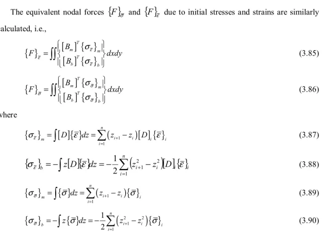
F=a −e−λ Slip, λ Load , F ∆λ ∆ F kFigure 3-3: Load-slip relationship for the shear connector [44].
The increment of shear force ∆F shown in Figure 3-3 can be related to the increment of slip ∆λ
as:
λ
∆ =∆F k (3.16)
where k is the slope of the load-slip curve and is given by:
λ
d dF k = (3.17) By differentiating Eq. 3.14, λ babe
k
=
− (3.18)and substituting in Eq. 3.16, the following relationship results:
λ
λ
∆
=
∆
F
abe
−b (3.19)For the element in Figure 3-2, the slip in the y and z directions can be written respectively as:
2 5 3 6 y z u u u u λ λ = − = − (3.20) or in incremental form:
2 5 3 6 y z u u u u λ λ ∆ = ∆ − ∆ ∆ = ∆ − ∆ (3.21)
where ∆ui is the increment of displacement due to an increment of shear force ∆Fi.
Note that in some cases the location of shear connectors may not coincide with the nodal points in the finite element mesh. In these cases, the actual connector is substituted by two equivalent connectors which are positioned at the nearest nodal points. The cross-sectional area of the substitute connectors is found by linearly interpolating the area of the actual connector. This procedure is akin to the determination of equivalent nodal forces in the customary finite element procedures.
In the non-linear incremental/iterative analysis procedure used in UMAR, increments of slip are summed up to obtain the total slip at any load level. Then, the shear force corresponding to the total slip is determined from Eq. 3.14, and the shear stiffness of the bar for the next iteration is calculated using Eq. 3.18. The axial stiffness of the bar is found the same way as for an ordinary truss element (see Section 3.1).
3.3 Refined quadrilateral plane element (RQD4)
This four-node quadrilateral element is geometrically isotropic, and its stiffness can be derived from the stiffness matrix of QUAD8, the eight-node isoparametric element. Element RQD4 has three degrees of freedom per node as illustrated in Figure 3-4, and its displacement functions can be derived from the displacement functions of QUAD8, also shown in Figure 3-4. Typical nodal displacements ui and vi in the x and y directions, respectively, are the same as in QUAD8, while
wi is a typical nodal-rotation normal to the plane of the element. This element was developed by
u4 v4 x y
8
7
6
5
4
3
2
1
η
ξ
u2 v24
3
2
1
η
ξ
w4 RQD4 QUAD8Figure 3-4: Elements QUAD8 and RQD4.
Using the kinematics relationship described below, the degrees of freedom in QUAD8 are related to the degrees of freedom in the new element. Consider side 1-2 of RQD4, and introduce a unit rotation w1 = 1 at node 1 as in Figure 3-5. The displacement normal to side 1-2, un, due to
this rotation can be expressed as a cubic polynomial similar to the lateral displacement function for an ordinary beam, i.e.,
(
)
2 2l
s
l
s
u
n=
−
−
(3.22)where s is a local co-ordinate running from node 1 to 2, and l is the length of side 1-2. For
2 l s= ,
( )
2 8 l n s l u = = − (3.23) Similarly, for w2 = 1:( )
2 8 l n s l u = = (3.24)Therefore, for end rotations w1 and w2, the normal displacement un is given by:
(
)
8 1 2 w w l un = − (3.25)(
)
(
)
2 1 2 1 sin 8 cos 8 x y n n w w u l w w u l θ θ − = − = (3.26)From Figure 3-5, sinθ =
(
y2−y1)
l and cosθ =(
x2−x1)
l, where xi, yi are the co-ordinates ofnode i (i = 1, 2). By substituting these quantities in Eq. 3.26, the total displacement components at
the middle of side 1-2 are:
(
) (
)(
)
(
) (
)(
)
2 1 1 2 2 1 5 2 1 1 2 2 1 5 2 8 2 8 u u y y w w u v v x x w w v + − − = − + − − = − (3.27)Equation 3.27 can be written in matrix form as:
1 1 5 1 5 2 2 2 1 1 0 0 2 2 1 1 0 0 2 2 u v a a u w v u b b v w − = − (3.28) where a=
(
y1−y2)
8 and b=(
x1−x2)
8. 1( )
n 11( )
2 2 s l s u l ω = − = − un 2 l ω1=1 ω2=0 θ sBy writing similar equations for the other mid-side nodes, the nodal displacements in QUAD8, {d}QUAD8, are related to the corresponding displacements in RQD4, {d}RQD4, as:
{ }
QUAD8[ ]
{ }
RQD4 16 1 16 12 12 1d × = T × d × (3.29)
where [T] is a 16 x 12 transformation matrix. In expanded form, Eq. 3.29 is given by:
−
−
−
−
−
−
−
−
=
4 4 4 3 3 3 2 2 2 1 1 1 4 4 4 4 3 3 3 3 2 2 2 2 1 1 1 1 8 8 7 7 6 6 5 5 4 4 3 3 2 2 1 12
1
0
0
0
0
0
0
0
2
1
0
0
2
1
0
0
0
0
0
0
0
2
1
2
1
0
2
1
0
0
0
0
0
0
0
0
2
1
0
2
1
0
0
0
0
0
0
0
0
0
2
1
0
2
1
0
0
0
0
0
0
0
0
2
1
0
2
1
0
0
0
0
0
0
0
0
0
2
1
0
2
1
0
0
0
0
0
0
0
0
2
1
0
2
1
0
1
0
0
0
0
0
0
0
0
0
0
0
0
1
0
0
0
0
0
0
0
0
0
0
0
0
0
1
0
0
0
0
0
0
0
0
0
0
0
0
1
0
0
0
0
0
0
0
0
0
0
0
0
0
1
0
0
0
0
0
0
0
0
0
0
0
0
1
0
0
0
0
0
0
0
0
0
0
0
0
0
1
0
0
0
0
0
0
0
0
0
0
0
0
1
w
v
u
w
v
u
w
v
u
w
v
u
a
a
b
b
a
a
b
b
a
a
b
b
a
a
b
b
v
u
v
u
v
u
v
u
v
u
v
u
v
u
v
u
(3.30)where ai=
(
xi−xi+1)
8 and bi=(
yi−yi+1)
8 for i=1,2,3; and a4=(
x1−x4)
8 and(
)
4 1 4 8
b = y −y .
Using the principle of virtual work, the stiffness [k*] and nodal load vector {f*} of RQD4 can be related to the corresponding matrices [k] and {f} of QUAD8 as:
[ ]
k* =[ ] [ ][ ]
T T k T (3.31) and{ }
*[ ]
{ }
12 16 16 1 12 1 T x x xf
=
T
f
(3.32)the desired stiffness and load matrices, it is possible to introduce further simplifications and to reduce the amount of calculations. The stiffness matrix, [k], is given by:
[ ] [ ] [ ][ ]
k
=
∫
B
TD
B
dV
(3.33)where, as usual, [B] is the strain-displacement matrix, [D] is the material matrix, and V is the
element volume. According to Eq. 3.31, [k*] can be written as:
[ ]
k
*=
[ ] [ ] [ ][ ]
T
T(
∫
B
TD
B
dV
)
[ ]
T
(3.34)Rewriting the above equation results in:
[ ]
k
*=
∫
[ ] [ ] [ ][ ][ ]
T
TB
TD
B
T
dV
(3.35) By letting[ ] [ ]
* 3 16 16 12 3 12x x xB
B
T
=
(3.36) then,[ ] [ ]
k* =∫
B* T[ ]
D[ ]
B*dV (3.37)Therefore, if matrix [B] of QUAD8 is transformed according to Eq. 3.36, then the stiffness matrix
of RQD4 can be derived from Eq. 3.37. By doing so, computation time is reduced, because Eq. 3.36 involves fewer multiplications. Several performance tests of element RQD4 can be found in [27] and [32].
3.4 Plate bending elements
Plate bending elements implemented in UMAR include the quadrilateral bending element (QBE) and the improved discrete Kirchoff quadrilateral (IDKQ).
3.4.1 Quadrilateral bending element (QBE)
This element is the quadrilateral version of the rectangular bending element developed by [47]. It was formulated by [11], and its performance has been reported to be satisfactory for moderate deviations from the rectangular shape. The general features of this element are briefly discussed below; complete details can be found in [11].
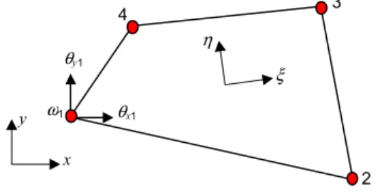
Element QBE, which is illustrated in Figure 3-6, is a four-node quadrilateral element with three degrees of freedom per node: the lateral displacement w, and the normal rotations w x∂ ∂
and ∂ ∂w y. The displacement function in terms of the natural co-ordinates ξ and η is given by:
[ ]
p
{ }
A
w
=
(3.38)and
{ }
A
is a vector that contains the polynomial coefficients. In this element, as in element RQD4, the geometry of the element is interpolated using the following relationships:(
)(
)
(
)(
)
4 1 4 1 1 1 1 4 1 1 1 4 i i i i i i i i x x y y ξξ ηη ξξ ηη = = = + + = + +∑
∑
(3.40)where x, y are the Cartesian co-ordinates of a general point, and ξ, η are the natural co-ordinates of the same point. Variables xi, yi, ξi and ηi are, respectively, the Cartesian and natural
co-ordinates of node i. Note that the summation is carried out over the four nodes of the element.
2 3 4 θx1 θy1 ω1 x y ξ η
Figure 3-6: Plate bending elements QBE and IDKQ.
3.4.2 Improved discrete Kirchhoff quadrilateral (IDKQ)
This type of element, like element QBE, is also a four-node quadrilateral element with three degrees of freedom at each node (see Figure 3-6). Element IDKQ is developed based on the Mindlin plate theory where the nodal rotations are defined independently of the transverse displacements [41]. The element shape functions are derived as the least square polynomial version of the customary Lagrange functions. Kirchhoff’s hypothesis is only applied to the Lagrange element at the rotational degrees of freedom θx and θy. This element is designed to
analyse thin plates where the transverse shear energy may be considered negligible compared to the bending one. The essential step in its formulation is the enforcement of the so-called Kirchhoff constraints
(
γ
yz =γ
zx =0)
at certain discrete points in such a manner that all shear-strain modes are totally suppressed. Feasible discrete points are the element nodes where the displacement modes are represented by the discrete values of the nodal displacements.The starting point in the formulation of the IDKQ is the Mindlin isoparametric finite element QUAD9 that accounts for shear deformations and requires only
C
( )0 -continuity. By imposing the Kirchhoff constraints on all shear strain modes, the 27 degrees of freedom (9 nodes x 3 dof pernode) of the QUAD9 may be transformed into 12 equivalent degrees of freedom (4 nodes x 3 dof per node) in the IDKQ element.
Similarly to the displacement transformation of RQD4, the aim of the transformation illustrated in Figure 3-7 is to derive the transformation matrix
[ ]
T
that maps the degrees of freedom of element QUAD9 into the equivalent degrees of freedom of element IDKQ, i.e.,{ }
9[ ]
{ }
18 1 18 12 12 1
QUAD IDKQ
d × = T × d × (3.41)
The nodal loads transformation may be also expressed by means of the transformation matrix
[ ]
T
:[ ]
{ }
9{ }
4 12 18 18 1 12 1 T QUAD IDKQT
×f
×=
f
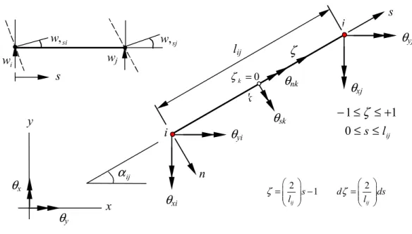
× (3.42)s
9s
n
s
n
s
n
n
η
, yη
, yξ
, x6
7
4
3
2
1
yiθ
i5
4
T
u X , u X , v Y , QUAD9 IDKQi
θ
xi yiθ
1
2
3
8
xiθ
Figure 3-7:Transformation of element QUAD9 into element IDKQ.
The transformation matrix
[ ]
T
in Eqs. 3.41 and 3.42 is determined by relating the mid-side and central nodes degrees of freedom of QUAD9 to the corner nodes degrees of freedom. This relation is established by imposing the Kirchhoff constraints so thatγ
z=
0
is exactly represented over the element. It should be noted that the element strains and the strain energy in QUAD9 depend only on rotations θx and θy, which are independent of the out-of-planeof freedom
w
i,w
,
xi=
θ
xi and w,yi=θ
yi (i = 1,…, 4) at the corners of the IDKQ element. Thistransformation is achieved by imposing the Kirchhoff constraints at the nodal points corresponding to the element sides and centrelines as follows:
Transverse shear strains
γ
yz andγ
zx vanish at the corner nodesxi xi
=
w,
θ
θ
yi =w,yi at nodesi
=
1
,
2
,
3
,
4
,
9
(3.43)Transverse shear strains
γ
sz (expressed in edge tangent co-ordinates
) vanish at the mid-side nodessk sk
=
w
,
θ
at nodesk
=
5
,
6
,
7
,
8
(3.44)Normal slopes
w
,
n=
θ
n of the cubic displacement function along the element sides are assumed to vary linearly(
ni nj)
nkθ
θ
θ
= + 2 1 at nodesk
=
5
,
6
,
7
,
8
for1
,
4
,
3
,
2
4
,
3
,
2
,
1
=
=
j
i
(3.45) In order to determine the transformation matrix[ ]
T
, the foregoing Kirchhoff constraints are applied along the element sides and centrelines making use of the corresponding co-ordinate transformations and a redefinition of the out-of-plane displacement field w, which must beassumed cubic in the edge tangent co-ordinate
s
along the element sides in order to be able to satisfy the Kirchhoff constraints as stated in Eqs. 3.43, 3.44 and 3.45, i.e.,(
)
[
]
3 3 2 ( ) 1 | 2 3 2 3 1 1 1 4 8 1, 2,3, 4 2,3, 4,1 i ij si side ij j sj w l w w i j ζ θ ζ ζ ζ ζ ζ ζ ζ θ = − + + − + − − + = = (3.46)where
ζ
and lij are respectively the natural co-ordinate and the length of the element side ij, andsi
θ
andθ
sj are the nodal tangential rotations along the element side ij at the end nodes i and j,respectively. The expression in Eq. 3.46 is obtained from a standard cubic Lagrangian function in natural co-ordinates
−
1
≤
ζ
≤
+
1
so thatζ
=
0
at the mid-side nodes. In order to express the rotationsθ
s=
w
,
s, the derivatives of wζ in Eq. 3.46 must be related to the physical co-ordinatek 0 = k ζ sj w, si w, i w ij l s≤ ≤ + ≤ ≤ − 0 1 1
ζ
ijα
j s x yθ
xθ
y 2 2 1 ij ij s d ds l l ζ = − ζ = wj lijζ
i nθ
xiθ
yiθ
skθ
nk sθ
xjθ
yjFigure 3-8: Co-ordinate transformation along of the side of a QUAD9 element.
The rotations
θ
sk=
w
,
sk(
k
=
5
,
6
,
7
,
8
)
at the mid-nodes of the QUAD9 element are thus obtained by differentiating Eq. 3.46 with respect tos
, i.e.,sj j ij si i ij sk
w
l
w
l
θ
θ
θ
4
1
2
3
4
1
2
3
−
+
−
−
=
(3.47) or in matrix form: − − − = nj sj j ni si i ij ij nk sk w w l lθ
θ
θ
θ
θ
θ
2 1 0 0 2 1 0 0 0 4 1 2 3 0 4 1 2 3 (3.48)where
i
=
1
,
2
,
3
,
4
,j
=
2
,
3
,
4
,
1
, andk
=
5
,
6
,
7
,
8
. Two other equations similar to Eq. 3.47 can be expressed for the centrelines of the QUAD9 element:6 6 68 8 8 68 9
4
1
2
3
4
1
2
3
x x xw
l
w
l
θ
θ
θ
=
−
−
+
−
(3.49) 5 5 57 7 7 57 94
1
2
3
4
1
2
3
y y yw
l
w
l
θ
θ
θ
=
−
−
+
−
(3.51)The set of six equations expressed in Eqs. 3.48, 3.49 and 3.51 provides the relationships needed to transform the rotational degrees of freedom
θ
xk andθ
yk(
k
=
5 K
,
,
9
)
of the QUAD9 element into the out-of-plane displacementsw
i and rotational degrees of freedomw
,
xi=
θ
xi andyi yi
w, =
θ
(
i
=
1 K
,
,
4
)
at the corners of the IDKQ element.Equation 3.48 needs to be expressed in terms of the element Cartesian co-ordinates x and y. The
transformation between side co-ordinates s,n and Cartesian co-ordinates x,y is achieved by means
of the Jacobian transformation matrices of each element side:
[ ]
−
=
=
ij ij ij ij ij r r s s ijy
x
y
x
J
α
α
α
α
cos
sin
sin
cos
,
,
,
,
(3.52)where
i
=
1
,
2
,
3
,
4
,j
=
2
,
3
,
4
,
1
, and[ ] [ ]
J
ij=
J
−ij1. Thus,[ ]
= yk xk ij nk sk Jθ
θ
θ
θ
(3.53) and Eq. 3.48 is expressed in Cartesian co-ordinates as:[ ]
[ ]
[ ]
[ ]
[ ]
− − − = ni ij xj ij j ni ij si ij i ij ij ij yk xk J J w J J w l l Jθ
θ
θ
θ
θ
θ
2 1 0 0 2 1 0 0 0 4 1 2 3 0 4 1 2 3 (3.55)1 1 2 2 3 3 4 4 5 5 6 6 7 7 8 8 9 9 0 0 1 0 0 0 0 0 0 0 0 0 0 1 0 0 0 0 0 0 0 0 0 0 0 0 0 0 0 0 1 0 0 0 0 0 0 0 0 0 1 0 0 0 0 0 0 0 0 0 0 0 0 0 0 0 1 0 0 0 0 0 0 0 0 0 0 1 0 0 0 0 0 0 0 0 0 x y x y x y x y x y x y x y x y x y θ θ θ θ θ θ θ θ θ θ θ θ θ θ θ θ θ θ − − − − − − = 9,1 9,2 9,3 9,4 9,5 9,6 10,1 10,2 10,3 10,4 10,5 10,6 11,4 11,5 11,6 11,7 11,8 11,9 12,4 12,5 12,6 12,7 12,8 12,9 13,7 13,8 13,9 13,10 13,11 13,12 0 0 0 0 0 0 1 0 0 0 0 0 0 0 0 0 0 1 0 0 0 0 0 0 0 0 0 0 0 0 0 0 0 0 0 0 0 0 0 0 0 0 0 0 0 0 0 0 0 0 0 T T T T T T T T T T T T T T T T T T T T T T T T T T T T T T − − 14,7 14,8 14,9 14,10 14,12 14,12 15,1 15,2 15,3 15,10 15,11 15,12 16,1 16,2 16,3 16,10 16,11 16,12 17,1 17,2 17,3 17,4 17,5 17,6 17,7 17,8 17,9 17,10 17,11 17,12 18,1 18,2 18,3 18,4 1 0 0 0 0 0 0 0 0 0 0 0 0 0 0 0 0 T T T T T T T T T T T T T T T T T T T T T T T T T T T T T T T T T T T 1 1 1 2 2 2 3 3 3 4 4 4 8,5 18,6 18,7 18,8 18,9 18,10 18,11 18,12 u v u v u v u v T T T T T T T θ θ θ θ (3.56) where
(
)
(
)
(
)
(
)
2 2 2 2 (9,1) 1.50 (1) (1) (9, 2) -0.75 (1) (1) (1) (9,3) -0.25 2.0 (1) - (1) (1) (9, 4) -1.50 (1) (1) (9,5) -0.75 (1) (1) (1) (9,6) -0.25 2.0 (1) - (1) (1) T a c T b a c T b a c T a c T b a c T b a c = ∗ = ∗ ∗ = ∗ ∗ = ∗ = ∗ ∗ = ∗ ∗ (3.57)(
)
(
)
(
)
(
)
2 2 2 2 (10,1) 1.50 (1) (1) (10, 2) 0.25 2.0 (1) - (1) (1) (10,3) 0.75 (1) (1) (1) (10, 4) -1.50 (1) (1) (10,5) 0.25 2.0 (1) - (1) (1) (10, 6) 0.75 (1) (1) (1) T b c T a b c T b a c T b c T a b c T a b c = ∗ = ∗ ∗ = ∗ ∗ = ∗ = ∗ ∗ = ∗ ∗ (3.58)(
)
(
)
(
)
(
)
2 2 2 2 (11, 4) 1.50 (2) (2) (11,5) 0.75 (2) (2) (2) (11, 6) 0.25 2.0 (2) - (2) (2) (11, 7) -1.50 (2) (2) (11,8) 0.75 (2) (2) (2) (11,9) 0.25 2.0 (2) - (2) (2) T a c T b a c T b a c T a c T a b c T b a c = ∗ = − ∗ ∗ = − ∗ ∗ = ∗ = − ∗ ∗ = − ∗ ∗ (3.59)(
)
(
)
(
)
(
)
2 2 2 2 (12, 4) 1.50 (2) (2) (12,5) 0.25 2.0 (2) - (2) (2) (12, 6) 0.75 (2) (2) (2) (12, 7) -1.50 (2) (2) (12,8) 0.25 2.0 (2) - (2) (2) (12,9) 0.75 (2) (2) (2) T b c T a b c T b a c T b c T a b c T a b c = ∗ = ∗ ∗ = ∗ ∗ = ∗ = ∗ ∗ = ∗ ∗ (3.60)(
)
(
)
(
)
(
)
2 2 2 2 (13,7) 1.50 (3) (3) (13,8) 0.75 (3) (3) (3) (13,9) 0.25 2.0 (3) (3) (3) (13,10) 1.50 (3) (3) (13,11) 0.75 (3) (3) (3) (13,12) 0.25 2.0 (3) - (3) (3) T a c T a b c T b a c T a c T a b c T b a c = ∗ = − ∗ ∗ = − ∗ ∗ − = − ∗ = − ∗ ∗ = − ∗ ∗ (3.61)(
)
(
)
(
)
(
)
2 2 2 2 (14, 7) 1.50 (3) (3) (14,8) 0.25 2.0 (3) (3) (3) (14,9) 0.75 (3) (3) (3) (14,10) 1.50 (3) (3) (14,11) 0.25 2.0 (3) - (3) (3) (14,12) 0.75 (3) (3) (3) T b c T a b c T a b c T b c T a b c T a b c = ∗ = ∗ ∗ − = ∗ ∗ = − ∗ = ∗ ∗ = ∗ ∗ (3.62)(
)
(
)
(
)
(
)
2 2 2 2 (15,1) 1.50 (4) (4) (15, 2) 0.75 (4) (4) (4) (15,3) 0.25 2.0 (4) (4) (4) (15,10) 1.50 (4) (4) (15,11) 0.75 (4) (4) (4) (15,12) 0.25 2.0 (4) - (4) (4) T a c T a b c T b a c T a c T a b c T b a c = ∗ = − ∗ ∗ = − ∗ ∗ − = ∗ = − ∗ ∗ = − ∗ ∗ (3.63)(
)
(
)
(
)
(
)
2 2 2 2 (16,1) 1.50 (4) (4) (16, 2) 0.25 2.0 (4) (4) (4) (16,3) 0.75 (4) (4) (4) (16,10) 1.50 (4) (4) (16,11) 0.25 2.0 (4) - (4) (4) (16,12) 0.75 (4) (4) (4) T b c T a b c T a b c T b c T a b c T a b c = − ∗ = ∗ ∗ − = ∗ ∗ = ∗ = ∗ ∗ = ∗ ∗ (3.64) 4 1 4 1 4 1 (17,1) 12.0 (1) (17, 2) (1) 2.0 (1) 2.0 (4) ( ) (17,3) (1) 2.0 (1) 2.0 (4) ( ) (17, 4) 12.0 (3) (17,5) (3) 2.0 (1) - 2.0 (2) ( ) (17,6) (3) i i i T d T d b b b i T d a a a i T d T d b b b i T d = = = = − ∗ ∆ ∗ = ∆ ∗ ∗ ∗ − ∗ + = −∆ ∗ ∗ ∗ − ∗ + = − ∗ ∆ ∗ = −∆ ∗ ∗ ∗ ∗ + = ∆ ∗∑
∑
∑
4 1 4 1 4 1 2.0 (1) 2.0 (2) ( ) (17,7) 12.0 (1) (17,8) (1) 2.0 (2) 2.0 (3) ( ) (17,9) (1) 2.0 (2) 2.0 (3) ( ) (17,10) 12.0 (3) (17,11) (3) 2.0 (4) 2.0 i i i a a a i T d T d b b b i T d a a a i T d T d b = = = ∗ ∗ − ∗ + = ∗ ∆ ∗ = ∆ ∗ ∗ ∗ − ∗ − = −∆ ∗ ∗ ∗ − ∗ − = ∗ ∆ ∗ = −∆ ∗ ∗ ∗ − ∗∑
∑
∑
4 1 4 1 (3) ( ) (17,12) (3) 2.0 (4) 2.0 (3) ( ) i i b b i T d a a a i = = − = ∆ ∗ ∗ ∗ − ∗ − ∑
∑
(3.65)4 1 4 1 4 1 (18,1) 12.0 (2) (18, 2) (2) 2.0 (1) 2.0 (4) ( ) (18,3) (2) 2.0 (1) 2.0 (4) ( ) (18, 4) 12.0 (4) (18,5) (4) 2.0 (1) - 2.0 (2) ( ) (18, 6) (4) 2 i i i T d T d b b b i T d a a a i T d T d b b b i T d = = = = ∗ ∆ ∗ = −∆ ∗ ∗ ∗ − ∗ + = ∆ ∗ ∗ ∗ − ∗ + = ∗ ∆ ∗ = ∆ ∗ ∗ ∗ ∗ + = −∆ ∗ ∗
∑
∑
∑
4 1 4 1 4 1 .0 (1) 2.0 (2) ( ) (18, 7) 12.0 (2) (18,8) (2) 2.0 (2) 2.0 (3) ( ) (18,9) (2) 2.0 (2) 2.0 (3) ( ) (18,10) 12.0 (4) (18,11) (4) 2.0 (4) 2.0 i i i a a a i T d T d b b b i T d a a a i T d T d b b = = = ∗ − ∗ + = − ∗ ∆ ∗ = −∆ ∗ ∗ ∗ − ∗ − = ∆ ∗ ∗ ∗ − ∗ − = − ∗ ∆ ∗ = ∆ ∗ ∗ ∗ − ∗∑
∑
∑
4 1 4 1 (3) ( ) (18,12) (4) 2.0 (4) 2.0 (3) ( ) i i b i T d a a a i = = − = −∆ ∗ ∗ ∗ − ∗ − ∑
∑
(3.66) with(
) (
)
[
]
[
]
[
]
[
]
[
]
4 4 2 2 1 1 4 4 1 1 4 4 1 1 ( ) ( ) - ( ); 1, 2,3, 4 ( ) ( ) - ( ); 2,3, 4,1 ( ) ( ) - ( ) (1) 2 (1) (4) ( ); (2) 2 (1) (4) ( ) (3) 2 (1) (2) ( ); (4) 2 (1) (2) ( ) 0.125 (3) - (1) (4) - (2 i i i i i i a i x i x j i b i y i y j j c i a i b i d b b b i d a a a i d b b b i d a a a i a a b b = = = = = = = = = = = = + − = + − = + − = + − ∆ =∑
∑
∑
∑
∑
∑
[
] [
][
]
{
) − a(4) - (2)a b(3) - (1)b}
(3.67)The stiffness transformation can be easily derived by substituting Eqs. 3.41 and 3.42 into the stiffness relationship for element QUAD9:
[ ]
[ ]{ }
{ }{ }
[ ]
[ ] [ ]
[ ]
9 9 9 9 QUADQUAD IDKQ QUAD IDKQ T QUAD
d
K T d = f ⇒ K = T K T
14243 (3.68)
As it can be observed, Eq. 3.68 does not change the element properties or its orientation in the global co-ordinate system. Rather, it represents a static condensation of the central and mid-node
degrees of freedom of the element QUAD9 in terms of the degrees of freedom at the corner nodes of the IDKQ element.
Further simplifications similar to that already shown for the RQD4 element are possible in order to reduce the amount of calculations required in the numerical integration process. These are achieved by rewriting
[ ]
K IDKQ as follows:[ ]
[ ] [ ]
(
9[ ][ ]
9)
[ ]
IDKQ T T QUAD QUAD K = T∫
B D B dV T (3.69) or[ ]
[ ] [ ]
9[ ][ ]
9[ ]
[ ] [ ][ ]
IDKQ T T TQUAD QUAD IDKQ IDKQ
K =
∫
T B D B T dV =∫
B D B dV (3.70) where[ ]
[ ]
9[ ]
3 12 3 18 18 12 IDKQ QUAD B × = B × T × (3.71)Finally, the stiffness matrix of the IDKQ element may be expressed as:
[ ]
12 12 1 1[ ] [ ] [ ]
1 1 IDKQ T IDKQ b IDKQ K B D B J d dξ η
+ + × − − =∫ ∫
(3.72)in which
[ ]
B IDKQ is the curvature-transformation matrix of the IDKQ element,[ ]
D
b is the bending elasticity matrix, and J is the determinant of the Jacobian matrix of the co-ordinate transformation. As it can be observed,[ ]
T 18 12× is not a square matrix, and it cannot be inverted. For this reason, the transformation of degrees of freedom by means of the matrix[ ]
T
can be only done from element QUAD9 to element IDKQ.The fact that the transformation matrix
[ ]
T 18 12× relates only to the rotational degrees of freedom makes it difficult to formulate the work equivalent nodal loads corresponding to distributed load. The cubic out-of-plane displacements w in Eq. 3.46 apply only on the border andcentre lines of the element. Therefore, it is not simple to formulate the work equivalent load vector for distributed loads. However, a lumped nodal load vector IDKQ
l
f can be employed as an approximation for the normal distributed load qTz =
[
qzi 0 0]
. For quadrilateral elements, bilinear shape functions can be used to represent the equivalent lumped nodal loads of the distributed load. For a rectangular element, the lumped nodal loads are:{
}
0 0 0 0 0 0 0 0 4 4 4 4 IDKQ e e e e l z A A A A f =q (3.73)where Ae is the area of the element. Since
w
is represented by a cubic interpolation as shown inEq. 3.46, a cubic polynomial expansion
N
c may be more consistent with the derivation of theequivalent nodal loads IDKQ c f :
{ }
e T IDKQ c c z e Af
=
∫
N q dA
(3.74) where[
]
{ }
a
N
Tc=
1
ξ
η
ξ
2ξη
η
2ξ
3ξ
2η
ξη
2η
3ξ
3η
ξη
3 (3.75)is a complete two-dimensional expansion from the Pascal Triangle, completed by the two bi-cubic extra terms
ξ
3η
andξ
3η
corresponding to the twelve generalised co-ordinates{ }
a
that must be exchanged with the twelve degrees of freedom{
d
IDKQ}
. Such exchange corresponds to the derivation of the shape function forw
in the Kirchhoff Plate Bending Theory. For a general quadrilateral shape of the element, numerical integration must be employed to obtain eitherIDKQ l
f or IDKQ c
f . Numerical experiments on element IDKQ show that the lumped nodal load vector IDKQ
l
f is a very good approximation for practical applications [41].
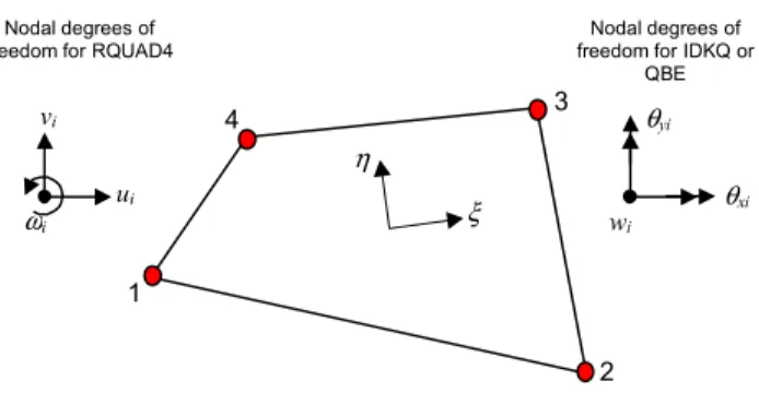
3.5 Quadrilateral facet shell element (QFSE)
The quadrilateral facet shell element QFSE, illustrated in Figure 3-9, is obtained by coupling the in-plane element RQUAD4 with the plate bending elements of Section 3.4 [27], [28] . The element has four nodes with six degrees of freedom per node: three displacements (u, v, w) and
three rotations (θx, θy, ωz). Because of material non-linearity, this element is an anisotropic shell
in which the membrane and bending actions are assumed to be coupled.
θxi θyi ωi ui vi Nodal degrees of freedom for RQUAD4
2 3 4 ξ η 1 wi Nodal degrees of freedom for IDKQ or
QBE
Figure 3-9: The facet shell element QFSE.
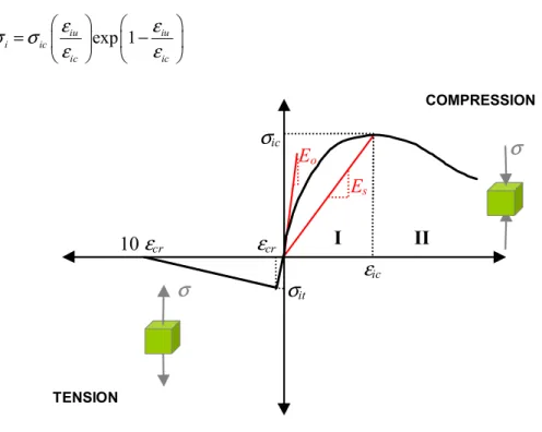
The strain {ε} at any point within the element is obtained from:
where {εo} is the vector of in-plane strains of the projection of a given point on the reference
plane, {χ} is the vector of curvatures due to bending, and z is the local z-co-ordinate through the
thickness of the element of the point under consideration (see Figure 3-10). The z-axis is
considered normal to the middle plane, and its origin coincides with the middle plane of the element. From basic theory:
{ }
ε =[ ]{ }
Bm dm (3.77){ }
χ
=
[ ]
B
b{ }
d
b (3.78)where subscripts m and b denote respectively membrane and bending actions. Equation 3.76 can
be re-written as:
{ }
[ ] [ ]
m[ ]{ }
m b b d B z B B d d ε = − = (3.79)By substituting [B] from Eq. 3.79 into the element stiffness equation, matrix [k] results in:
[ ]
[ ] [ ][ ]
[ ] [ ][ ]
[ ] [ ][ ]
2[ ] [ ][ ]
[ ] [ ]
[ ] [ ]
T T m m m b mm mb T T bm bb b m b b B D B z B D B k k k dV k k z B D B z B D B − = = − ∫
(3.80)The diagonal terms in Eq. 3.80 are the respective stiffness matrices of element RQUAD4 and the plate bending element. The off-diagonal terms are the coupling matrices, which are non-zero if the material properties are not symmetric with respect to the middle surface of the shell. This situation can occur when yielding and/or cracking takes place in some fibres above or below the middle surface and not in others. In program UMAR, plate and shell elements are divided into layers of different materials, as illustrated in Figure 3-10. Each layer is assumed to be in a state of plane stress. Within the thickness of each layer, the stresses and material properties are assumed to be constant.
z
1
2
3
Reference surface Body layerh
C o ns ta nt T hi c k n es st
z
z
topz
bottom Element nodeFigure 3-10: Layered shell element.
In evaluating the sub-matrices that comprise the stiffness matrix [k] in Eq. 3.80, the volume
integral is split into a summation over the number of layers through the thickness and an area integral over the surface of the element. For example,
[ ]
[ ] [ ][ ]
T[ ] [ ] [ ]
T m m m m mm z k = B D B dV = B D dz B dxdy ∫
∫∫
∫
(3.81)The line integral along the thickness of the shell of Eq. 3.81, denoted by [D]mm, is calculated in
the following fashion:
[ ]
[ ]
(
1)
[ ]
1 n i i mm i i z D D dz z+ z D = =∫
=∑
− (3.82)where zi+1 and zi are the z co-ordinates of the top and bottom surfaces of layer i, and n is the total
number of layers in a given element. The constitutive matrix [D]i for each layer will depend upon
the material forming that layer. The remaining sub-matrices in Eq. 3.80 are evaluated in a similar way, the line integral for the remaining terms resulting in:
[ ]
[ ]
(
2 2)
[ ]
1 1 1 2 n i i mb i i z D z D dz z+ z D = =∫
= −∑
− (3.83)[ ]
[ ]
(
)
[ ]
i n i i i z bbz
D
dz
z
z
D
D
∫
∑
= +−
=
=
1 3 3 1 23
1
(3.84) The equivalent nodal forces{ }
F
σ and{ }
F
ε due to initial stresses and strains are similarlycalculated, i.e.,
{ }
[ ]
{ }
[ ]
{ }
T m m T b b B F dxdy B ε ε ε σ σ = ∫∫
(3.85){ }
[ ] { }
[ ] { }
T m m T b b B F dxdy B σ σ σ σ σ = ∫∫
(3.86) where{ }
[ ]{ }
(
1)[ ] { }
1 n i i m i i i D dz z z D ε σ ε + ε = =∫
=∑
− (3.87){ }
[ ]
{ }
(
)
[ ]
i{ }
i n i i i bz
D
ε
dz
z
z
D
ε
σ
ε∫
∑
= +−
−
=
−
=
1 2 2 12
1
(3.88){ }
{ }
(
1){ }
1 n i i m i i dz z z σ σ σ + σ = =∫
=∑
− (3.89){ }
{ }
(
2 2)
{ }
1 1 1 2 n i i b i i z dz z z σ σ σ + σ = = −∫
= −∑
− (3.90)3.6 Solid isoparametric element
Program UMAR has two hexahedral isoparametric elements of the “serendipity” family (i.e., containing boundary nodes only): a linear brick element (8 nodes) and a quadratic brick element (20 nodes), see Figure 3-11.
8 nodes (linear)
20 nodes (quadratic)
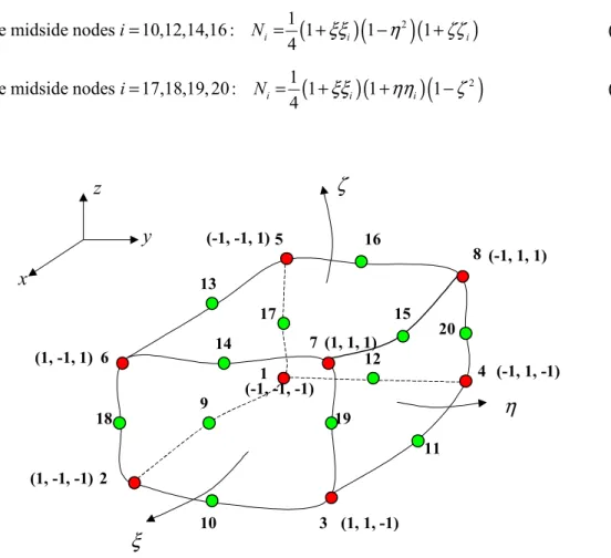
Figure 3-11: Hexahedral elements of the “serendipity” family implemented in UMAR.
where i ranges over the number of nodes in the element. The shape functions Ni are functions of
the isoparametric coordinates ξ, η, and ζ, and the faces of the element lie at ξ = ±1, η= ±1, and 1
ζ = ± , respectively (see Figure 3-12). The node numbering convention used in Figure 3-12 is that of corner nodes being numbered first, followed by mid-side nodes for the second-order element (20-node brick element).The shape functions for the 8-node brick element can be summarized in:
(
)(
)(
)
1 1 1 1 8 i i i i N = +ξξ +ηη +ζζ (3.92)where ξi, ηi, and ζi denote the natural co-ordinates of the ith node. The shape functions of the
20-node brick can be grouped as follows:
(
)(
)(
)(
)
1
For the corner nodes 1, 2, ,8 : 1 1 1 2
8
i i i i i i i
i= K N = +ξξ +ηη +ζζ ξξ ηη ζζ+ + − (3.93)
(
2)
(
)(
)
1
For the midside nodes 9,11,13,15 : 1 1 1 4
i i i
i= N = −ξ +ηη +ζζ (3.94)
(
)
(
2)
(
)
1
For the midside nodes 10,12,14,16 : 1 1 1 4
i i i
i= N = +ξξ −η +ζζ (3.95)
(
)(
)
(
2)
1
For the midside nodes 17,18,19, 20 : 1 1 1 4 i i i i= N = +ξξ +ηη −ζ (3.96)
![Figure 3-3: Load-slip relationship for the shear connector [44].](https://thumb-eu.123doks.com/thumbv2/123doknet/14198571.479529/14.918.191.557.110.270/figure-load-slip-relationship-shear-connector.webp)