HAL Id: hal-02639065
https://hal.archives-ouvertes.fr/hal-02639065
Submitted on 28 May 2020HAL is a multi-disciplinary open access archive for the deposit and dissemination of sci-entific research documents, whether they are pub-lished or not. The documents may come from teaching and research institutions in France or abroad, or from public or private research centers.
L’archive ouverte pluridisciplinaire HAL, est destinée au dépôt et à la diffusion de documents scientifiques de niveau recherche, publiés ou non, émanant des établissements d’enseignement et de recherche français ou étrangers, des laboratoires publics ou privés.
Sensitivity computations by algorithmic differentiation
of a high-order cfd code based on spectral differences
José Cardesa, Christophe Airiau
To cite this version:
José Cardesa, Christophe Airiau. Sensitivity computations by algorithmic differentiation of a high--order cfd code based on spectral differences. Aerospace Europe conference 2020, Feb 2020, Bordeaux, France. pp.0. �hal-02639065�
OATAO is an open access repository that collects the work of Toulouse
researchers and makes it freely available over the web where possible
Any correspondence concerning this service should be sent
This is a Publisher’s version published in:
http://oatao.univ-toulouse.fr/25696
To cite this version:
Cardesa, José I.
and Airiau, Christophe
Sensitivity computations by
algorithmic differentiation of a high-order cfd code based on spectral
differences. (2020) In: Aerospace Europe conference 2020, 25 February 2020 -
1
INSTRUCTIONS PAPER ID. 019
SENSITIVITY COMPUTATIONS BY ALGORITHMIC DIFFERENTIATION OF A
HIGH-ORDER CFD CODE BASED ON SPECTRAL DIFFERENCES
José I. Cardesa(1), Christophe Airiau(2)
(1) IMFT, 2 Allée du Professeur Camille Soula, 31400 Toulouse, FRANCE, Email: [email protected]
(2) IMFT, 2 Allée du Professeur Camille Soula, 31400 Toulouse, FRANCE, Email: [email protected]
KEYWORDS: computational fluid dynamics,
automatic differentiation, sensitivity analysis, flow control, optimization.
ABSTRACT:
We compute flow sensitivities by differentiating a high-order computational fluid dynamics code. Our fully discrete approach relies on automatic differentiation (AD) of the original source code. We obtain two transformed codes by using the AD tool Tapenade (INRIA), one for each differentiation mode: tangent and adjoint. Both differentiated codes are tested against each other by computing sensitivities in an unsteady test case. The results from both codes agree to within machine accuracy, and compare well with those approximated by finite differences. We compare execution times and discuss the encountered technical difficulties due to 1) the code parallelism and 2) the memory overhead caused by unsteady problems.
1. INTRODUCTION
Numerical codes in engineering and physical sciences are most often used to approximate the solution of governing equations on discretized domains. A natural step beyond obtaining solutions in specific conditions is to seek those conditions that modify the solution towards a specific goal, either for optimization or control purposes. In this context, gradient-based methods play an important role. They require invariably the computation of derivatives, a task that can be automated by Automatic Differentiation (AD) tools. In short, AD augments outputs 𝑌" from inputs 𝑋$ into a
“differentiated” code that additionally computes some derivatives 𝑑𝑌"/𝑑𝑋$ requested by the user. AD
provides two main modes, the tangent/direct/forward mode and the adjoint/reverse/backward mode. If 1 ≤ 𝑖 ≤ 𝑝 and 1 ≤ 𝑗 ≤ 𝑞 bound the size of the output and input spaces, respectively, then the tangent mode is most efficient when 𝑞 ≪ 𝑝 while the adjoint mode is the only realistic option for 𝑝 ≪ 𝑞.
Two features of high-performance codes used in industry and academia complicate the process of
computing derivatives with AD: parallel communications and unsteady computations. The tangent mode of AD can deal with these features quite easily, while the adjoint mode of AD is affected by these features as it is based on reversal of the data-flow of the primal code [12]. Unfortunately, many real-life applications require computing derivatives of relatively few outputs (cost functions, constraints…) with respect to many inputs (state variables, design parameters, mesh coordinates…). Tangent AD is out of question in such cases since 𝑝 ≪ 𝑞. As long as the adjoint mode provided by AD tools did not address these serious limitations, most studies [1-3] circumvented them by using the following strategies:
• Applying AD on selected parts of the code without MPI calls and manually assembling the differentiated routines to obtain a correct adjoint code
• Restricting the use of AD to code solving problems that are either stationary of forced to become stationary. As an exception, earth sciences have long used adjoints of unsteady simulations [4-5], pioneering the so-called checkpointing schemes that we advocate here.
In this talk, we report on the outcome of exploiting the recently acquired maturity of AD tools [6] at differentiating parallel code in adjoint mode by automatic inversion of the MPI communication layer [7] while handling the cost of an unsteady computation.
2. SOFTWARE USED
We now provide details related to the flow solver and the AD tools used in our study.
2.1. Flow solver
The code under consideration in the present study – hereafter the primal code – is a computational fluid dynamics (CFD) solver that integrates the governing equations for compressible fluid flow. It belongs to a recent trend of CFD codes that use a high-order spatial discretization adapted to
compressible/incompressible flow computations on complex geometries modeled by unstructured meshes. This makes them suitable candidates to become industrial tools in the near future [8]. Our application code is Jaguar [9-10], a solver for aerodynamics applications developed to suit the future needs of the aerospace industry. The code is written following features from the Fortran 90 standard onward, with a zero-halo partitioning scheme and MPI-based parallelization.
2.2. AD tool
AD can be based on two working principles: operator overloading (OO) or source transformation (ST). The OO approach barely modifies the primal code: the data-type of numeric variables is simply modified to contain their derivative in addition to their primal value, while arithmetic operations are overloaded to act on both components of the variables. While the debate is still active, it is generally agreed that ST AD tools require a much heavier development, which is in general paid back by a better efficiency of the differentiated code mostly in terms of memory consumption. Benchmark tests have pointed out a tendency for OO-differentiated codes to be more memory demanding and somewhat slower than their ST counterparts [2]. On the other hand, the higher flexibility of the OO model makes it almost readily applicable to languages with sophisticated constructs, such as C++ or Python, for which no ST tool exists to date. For a given application, the choice between AD tools based on ST or OO is dictated by these constraints: with Jaguar being written in Fortran, ST appears to be the natural choice. Moreover, for the size and number of time steps of our targeted applications, it is essential to master the memory footprint of the final adjoint code. For this study, we have selected the ST- based AD tool Tapenade [11], developed by INRIA.
2.3. AD of very long time-stepping sequences
The adjoint mode of AD leads to a code which executes the differentiated instructions in the reverse order of the primal code. However, these differentiated instructions (the “backward sweep”) use partial derivatives based on the values of the variables from the primal code. The primal code, or something close to it, must therefore be executed beforehand, forming the “forward sweep”. As codes generally overwrite variables, a mechanism is needed to recover values overwritten during the forward sweep, as they are needed during the backward sweep. Recovering intermediate values can be done either by recomputing them at need, from some stored state, or by storing them on a stack during the forward sweep and retrieving them during the backward sweep. Neither option scales well on large codes, either with a memory use that
grows linearly with the primal code run time, or with an execution time that grows quadratically with the primal code run time. We envision applications with 105 to 106 time steps to integrate the fluid flow
equations. The classical answer to this problem is a memory-recomputation trade off known as “checkpointing” [12]. A well-chosen checkpointing strategy can lead to execution time and memory consumption of the adjoint code that grow only logarithmically with the primal code run time.
A checkpointing strategy is constrained by the structure of the primal code. Checkpointing amounts to designating (nested) portions of the code, for which we are ready to pay duplicate execution to gain memory storage of its intermediate computations. These portions must have a single-entry point and a single exit point, for instance procedure calls or code parts that could be written as procedures. For this reason, one cannot in practice implement the theoretical optimal checkpointing scheme, which is defined only on a fixed-length linear sequence of elementary operations of similar cost and nature. A checkpointing scheme on a real code can still achieve a logarithmic behavior, but in general below the theoretical optimal. Moreover, since checkpointed portions are supposed to be executed twice or more, they must be “reentrant”: it must be possible to re-create the exact machine state at their entry point, and running them twice must not alter the rest of the execution. As a consequence, a checkpointed portion of code must always contain both ends of an MPI communication, and similarly both halves of a non-blocking MPI communication [13].
Time-stepping simulations are more fortunate: at the granularity of time steps, the code is indeed a fixed-length sequence of elementary operations of similar cost and nature. The binomial checkpointing scheme [14] exactly implements the optimal strategy in that case, and Tapenade applies it when requested. A checkpointing strategy is also constrained by the characteristics of the storage system. The binomial strategy assumes a uniform and negligible cost for storing and retrieving the memory state before checkpoints (“snapshots”). This is in reality never the case. New research [15] looks for checkpointing strategies that take this memory cost into account, as well as different access times for different memory levels.
In general, few studies confront unsteady problems directly, and most works reported in the literature focus on problems around a fixed-point solution. Convergence towards that fixed steady state is often enforced by means of implicit iterative schemes with preconditioning. Few iterations are necessary, and only the final converged state
3 requires storage before computing the inverted set of instructions. Consequently, memory and computational overhead are kept low. It is unfortunate, however, that many problems of industrial relevance are inherently unsteady. In acoustics and combustion, for instance, unsteadiness simply cannot be ignored, which is what motivates the present study.
2.4. Parallel communications
An additional challenge arises when the code to be inverted by the AD tool contains message-passing instructions, which also need to be invoked in inverted order. Much conceptual work has been devoted to AD of MPI code [16-20]. However, it is with the recent advent of the Adjoinable MPI library [7] that several AD tools (Adol-C, Rapsodia, dco, OpenAD, Tapenade) support AD of code containing MPI calls. Related projects include the Adjoint MPI library [18,20,21] compatible with the dco suite of AD tools, and CoDiPack [22] for C++ code - both based on OO. The automatic inversion of MPI calls necessary to derive a parallel adjoint code can thus be performed by three tools. In [21], the CFD code OpenFOAM was adjointed with the combination of dco/c++ and Adjoint MPI. CoDiPack was used to adjoint the CFD code SU2 [23]. To our knowledge, these are the most similar studies to ours in terms of letting the AD tool handle the parallel communication layer automatically - yet without solving a time-dependent problem.
Avoiding MPI idioms in code fed to an AD tool is an attractive choice. Individually differentiated routines can be manually assembled into an adjoint code that preserves the often heavily optimized parallel communications layer of the primal code. A disadvantage of this approach is the increased workload incurred every time a different problem is tackled, where the optimization concerns different quantities from those previously considered. A certain degree of freedom in choosing the cost function and automation in assembling differentiated procedures has been achieved in [1]. Alternatively, [24] has presented the transposed forward-mode algorithmic differentiation to take advantage of those code portions featuring symmetric properties in order to obtain adjointed code using the forward-mode AD. Either way, handling MPI calls differently from the rest of the code contradicts the ultimate goal of AD, which is full automation of the differentiation process regardless of the programming features actually used in the primal code. It is true, however, that each specific library that involves side-effects raises new issues, limitations, and challenges that cannot be readily solved by AD tools. Given the efforts that have been devoted towards making MPI calls compatible with AD tools [16-20], we aim to test and
document the outcome of letting the AD tool handle them alone. In this respect, our work intends to provide a proof of concept illustrating that the route followed, which on the whole has been avoided in the literature, is in fact practicable.
3. TEST CASE
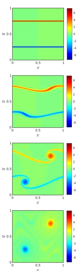
We consider a viscous, two-dimensional incompressible flow in a square periodic domain spanning 𝐿 = 1 in the streamwise (𝑥) and vertical (𝑦) directions. The velocity field at the initial instant 𝑡5 is given by
𝑢 = 𝑈 tanh[𝑟(𝑦 − 1/4)], 𝑦 ≤ 1/2 (1) 𝑢 = 𝑈 tanh[𝑟(3/4 − 𝑦)], 𝑦 > 1/2 (2) 𝑣 = 𝑈𝛿 sin[2𝜋(𝑥 + 1/4)], (3)
where all quantities are made non-dimensional with 𝐿 and the streamwise reference velocity 𝑈5= 1 as
follows:
𝑡 = 𝑡̃𝑈5/𝐿, 𝑦 = 𝑦M/𝐿, 𝑥 = 𝑥M/𝐿, 𝑈 = 𝑈N/𝑈5, 𝑟 = 𝑟̃𝐿. (4)
The parameters of the problem are 𝑈, 𝑟 and 𝛿. These are the streamwise velocity amplitude, the shear parameter and the ratio of vertical to streamwise velocity amplitudes, respectively. We set 𝛿 = 0.05 for the remainder of the study so that is is no longer a free parameter. We analyse the evolution of the overall enstrophy Ω, defined as Ω = ∫ ∫ TU𝜔WU 𝑑𝑥 𝑑𝑦, T 5 T 5 (5) where 𝜔W= 𝜕Y𝑣 − 𝜕Z𝑢 is the vorticity. It can be
readily shown from Eqs. 1-3 and Eq. 5 that at 𝑡 = 𝑡5,
Ω = 𝑈U[6𝑟 tanh ]^ _` − 2𝑟 tanh a]^ _` + 3𝛿 U𝜋Ub /3 (6)
and we choose 𝑟 = 40 with 𝑈 = 1 to yield an initial enstrophy level Ω^cd= 53.36 which we set as a
constraint for all 𝑟. This implies 𝑈 is a function of 𝑟 only, determined by re-arranging Eq. 6 as follows:
𝑈(𝑟) = e3Ω^cd/(6𝑟 tanh(𝑟/4) − 2𝑟 tanha(𝑟/4) +
3𝛿U𝜋U )fT/U. (7)
The Reynolds number is 𝑅𝑒5= 𝑈5𝐿/𝜈 = 1.176 ×
10_. We show the spatial distribution of 𝜔
W at four
different instants obtained with 𝑟 = 160 on Fig. 1. The dependence of Ω on time and 𝑟 is clear from Fig. 2.
Figure 1 Spatial distribution of out-of-plane vorticity 𝜔W/lΩ^cd at instants 𝑡lΩ^cd= {0,7,10,23} from top
to bottom, with 𝑟 = 160.
Figure 2 Time dependence of 𝛺 at three different values of shear parameter 𝑟. Results obtained with codes Jaguar and MatSPE. The legend includes the number of Fourier modes used in each direction for the MatSPE simulation (of which 1/3 are zero- padded for dealiasing), while the JAGUAR data includes parameter 𝑝 which is the selected order of the spatial discretization of the spectral difference scheme. The grid used in the JAGUAR simulation is a 72 × 72 structured mesh which, together with the setting 𝑝 = 4, yields 360 degrees of freedom (DoF) per spatial direction. So we are effectively comparing 2562 DoF with MatSPE against 3602
DoF with JAGUAR.
The incompressible 2D Navier-Stokes equations are solved with the initial and boundary conditions outlined above using JAGUAR on a structured mesh with 72 × 72 square elements. The Mach number is set to zero to approach, as much as possible, incompressibility. The solution and flux points are located following Gauss-Lobatto- Chebyshev and Legendre collocation, respectively, and the CFL is kept constant at 0.5. The fluxes at the cell faces are computed with the Roe scheme. The temporal integration is done with a six-stage, fourth-order low-dissipation low-dispersion Runge- Kutta scheme optimized for the spectral difference code using the procedure in [25]. We use an in- house, fully spectral code (MatSPE) designed for periodic incompressible viscous flows to solve the same test case and validate Jaguar. The output of the two codes is compared on Fig. 2, showing that the agreement between the codes is extremely good.
We define the following cost function
𝐽 = ∫ Ω(𝑡) 𝑑𝑡5q . (8)
Its derivative with respect to 𝑟 will be the target sensitivity we compute by means of AD. From a physical point of view, Ω(𝑡) is directly proportional to the rate of kinetic energy dissipation in the flow due
0 5 10 15 20 25 30 35 0.1 0.2 0.3 0.4 0.5 0.6 0.7 0.8 0.9 1 r=40, 384x384, MatSPE r=80, 384x384, MatSPE r=160, 384x384, MatSPE r=40, 72x72, p=4, JAGUAR r=80, 72x72, p=4, JAGUAR r=160, 72x72, p=4, JAGUAR
5
to the action of viscosity. Hence, the area under a curve of Ω(𝑡) on Fig. 2 for a given time interval is a proxy for the kinetic energy dissipated by the flow during that time. It may be argued that since our numerical experiments only target 𝑑𝐽/𝑑𝑟, it is pointless to use adjoint-mode AD because 𝑟 is a scalar. One must bear in mind, however, that the final application of our study is to compute sensitivities of some 𝐽 with respect to many inputs. Restricting the number of inputs to one in the sequel is only a convenient way to validate our proposed work flow and the AD derivatives, as well as to compare and study performance.
The computation of 𝐽 in the primal code is carried out by adding a contribution to the time integral at each new time step in a running sum fashion, using a simple trapezoidal rule. Such a framework is convenient to illustrate the fundamental issue of adjoint-mode AD that we already described in section 2.3. The tangent-differentiated code accumulates contributions of each time step to 𝑑𝐽/𝑑𝑟, along with the primal time-stepping sequence, i.e. in the same order. This is conceptually simple: once we reach the iteration corresponding to 𝑡 = 𝑇 (which we will call iteration number 𝑁), both 𝐽 and 𝑑𝐽/𝑑𝑟 are known and the program can end. In contrast, the adjoint- differentiated code will first run an initial forward sweep that will integrate the Navier-Stokes equations from 𝑡 = 0 to the iteration 𝑁 of the time- stepping loop, chiefly to generate the final state of the program variables. Only then can the backward sweep of the adjoint code start to accumulate derivatives, computing the sensitivity of 𝐽 with respect to the state variables at iteration 𝑁 − 1, and carry on stepping back in time to finally obtain 𝑑𝐽/𝑑𝑟 when 𝑡 = 0 is reached. In order to provide intermediate values from the forward sweep to the backward sweep in the correct order (i.e. reversed), a combination of stack storage and additional forward recomputation is needed, making a good checkpointing scheme essential. The recomputations and stack use will inevitably imply that one run of the adjoint code requires significantly more memory and execution time than the tangent code. We thus expect the tangent code to still outperform the adjoint code when 𝑝 = 𝑞 or when 𝑞 is only a few times larger than 𝑝, but the adjoint code will definitely outperform the tangent code when 𝑝 ≪ 𝑞, which is the case in many applications.
4. SENSITIVITY VALIDATIONS WITH FINITE DIFFERENCES
The estimates of a given sensitivity computed with tangent- or adjoint-mode AD codes should agree almost to machine precision, as they result from the same computation modulo associativity- commutativity. In contrast, the reference value
against which to validate the sensitivity is obviously a finite-difference (FD) estimate, which is subject to errors due to the contribution of higher derivatives. For the viscous test case, we compute our FD estimates with two independent realizations at 𝑟 and 𝑟 + 𝑑𝑟, where 𝑑𝑟/𝑟 = 10tu. We thus expect an
agreement between FD and AD derivatives up to more or less half of the decimals, whereas we expect a much better agreement between tangent AD and adjoint AD derivatives.
5. DIFFERENTIATION WORK FLOW
We adopted the following work flow with regards to the Jaguar flow solver, the working principles of Tapenade and the Adjoinable MPI library:
A. Identify the part of the code that computes the function to differentiate, exactly from the differentiation input variables to the differentiation output, and make it appear as a procedure (the “head” procedure). This may require a bit of code refactoring. The differentiation tool must be given (at least) this root procedure and the call tree below it.
B. Migrate all MPI calls to Adjoinable MPI, whether AD will be applied in tangent or in adjoint mode. This involves two steps. First, as Adjoinable MPI does not support all MPI communication styles (e.g. one-sided), the code must be transformed to only use the supported styles, which is a reasonably large subset. Second, effectively translate the MPI constructs into their Adjoinable MPI equivalent, which occasionally requires minor modifications to the call arguments. As Adjoinable MPI is just a wrapper around MPI, the resulting code should still compile and run, and it is wise to test that.
C. Provide the AD tool with the source of the head procedure and of all the procedures that it may recursively call, together with the specification of the differentiation input and output variables. Then differentiate, after which two steps follow. First, fix all issues signaled by the AD tool, e.g. unknown external procedures or additional info needed, and validate the differentiated code. Second, address performance issues and in particular optimize the checkpointing strategy by adding AD-related directives to the source. This may also involve special treatment of linear algebra procedures such as solvers.
6. RESULTS
The temporal integration of the equations of motion is carried out from 𝑡 = 0 to the 𝑛 − 𝑡ℎ iteration of the time integration loop in Jaguar, with 𝑛 = 6.8 × 10u.
With the CFL setting outlined in section 3, this number of time steps corresponds to 𝑡lΩ^cd= 19.8,
which from Fig. 1 can be seen as the time when the decay of Ω becomes slow for all three values of 𝑟. The value of 𝑑𝐽/𝑑𝑟 is given in Tab. 1, where the results from FD, tangent-mode AD and adjoint- mode AD are all gathered. The agreement between FD-based sensitivities and AD validates the differentiation procedure.
Table 1 𝑑𝐽/𝑑𝑟 computed with three different methods, for the time integration interval between 𝑡 = 0 and 𝑡 = 𝑇 (6.8 × 10utime steps). Viscous test
case with 𝑟 = 160, run with 16 parallel processes. Differentiation method Sensitivity 𝑑𝐽/𝑑𝑟
FD (MPI) -0.22002254
Tangent AD (AMPI) -0.22002394265381 Adjoint AD (AMPI) -0.22002394265861
The agreement between the two AD-based sensitivities is excellent, within round-off error of double precision arithmetic. It was expected in case of correct differentiation by Tapenade, but nevertheless it is puzzling when comparing the drastic differences between the two differentiated codes. The fact that the adjoint-differentiated code outputs the correct answer after carrying out the time-stepping loop backwards confirms the absence of any stability or convergence issues related to inverting the instructions of a code that integrates in time a reversible and dissipative system. More specifically, there is no issue of numerical instability caused by a term with negative diffusivity.
The time required for the various computations is shown on Tab. 2. A factor of two is indicated for the FD computation, given that two runs of the primal code are required. The computations are run on 16 Intel(R) Xeon(R) Gold 6140 processors at 2.30GHz. The Intel Fortran compiler version 18.0.2 is used, with identical optimization flags for all codes: -xCORE-AVX2 -ipo -O3 -qopt-malloc-options=3. It appears that the tangent-mode AD can be faster than two runs of the primal code, requiring 1.7 times the execution time of the primal code. The higher accuracy of sensitivity computations from tangent- mode AD thus comes with the added benefit of a faster computation than that of FD. Furthermore, each additional cost function differentiated with respect to 𝑟 will require an additional FD computation, whereas the cost of each new sensitivity with respect to 𝑟 will keep the cost of the tangent-mode execution constant. We note in passing that the FD computation is based on the
MPI code before the modifications of step B. outlined in section 5, so that the tangent-mode AD is faster than the FD computations despite the move from MPI to Adjoinable MPI. This indicates that the cost of this additional wrapper on top of the MPI library is negligible.
Table 2 Same as Tab. 1, but showing execution times normalized by the primal code execution time.
Differentiation method Normalized run time
FD (MPI) 1 (x2)
Tangent AD (AMPI) 1.7
Adjoint AD (AMPI) 15.4
Tab. 2 also shows the slowdown factor of the adjoint code, which is 15.4 and deserves some discussion. An initial experiment without any specific checkpointing scheme simply ran out of memory after only less than a hundred timestepping iterations. Therefore, binomial checkpointing is unavoidable. It accounts for a significant part of this adjoint slowdown: since we chose to allow for 80 snapshots for binomial reversal of 6.8 × 10u time
steps, the binomial model tells us this costs an average 3.9 extra recomputations per time step. This leaves us with roughly an 11-fold slowdown to account for, which is still higher than expected. There is certainly still room for improvement of our current checkpointing scheme. We still have to investigate the impact of the very deep call tree inside each time step, or the possibility to improve the time to write and read memory snapshots. Both the tangent and the adjoint codes produced by Tapenade received no further optimization other than compilation options. Nevertheless, with their present performance, the adjoint code is already preferable to the tangent code as soon as the number of input variables, with respect to which we request sensitivities, goes over 15.
7. CONCLUSIONS AND FUTURE WORK
A CFD code with a high-order spatial discretization based on spectral differences and an optimized parallel communications layer has been automatically differentiated by letting the AD tools (Tapenade and Adjoinable MPI) handle the communications layer in an automated way. In adjoint mode, the inversion of the communications during the backward sweep was found to produce correct code which could execute in 15 times the primal code execution time. The computational overhead is to a large extent the consequence of having to resort to binomial checkpointing to trade storage for computational time in order to invert a temporal integration loop with a number of iterations of the order of 106. We have presented a detailed
outline of the code modifications required to achieve the correct differentiation of the parallel code.
7
A viscous flow test case was treated. Even though it is a physically dissipative system, it has been computed using the backward mode of AD without running into stability issues, and yielding the correct derivative at the end of the computation. The run time for the tangent-differentiated code was 1.7 times slower than a single run of the primal. It is therefore readily superior to finite difference approximations even for single derivative computations. A natural further step would involve embedding the derivative solver into an optimal control loop. The strength of a code such as Jaguar lies in its ability to handle acoustics problems, such as the noise radiated by the wake of an object during a given time. Optimization in this type of problems constitutes an interesting perspective to the present work.
8. ACKNOWLEDGEMENTS
We thank Laurent Hascoët (INRIA Sophia-Antipolis) for the help provided with Tapenade. This work has been financed by a grant from the STAE Foundation for the 3C2T project, managed by the IRT Saint- Exupéry. J.I.C. acknowledges funding from the People Program (Marie Curie Actions) of the European Union’s Seventh Framework Program (FP7/2007-2013) under REA grant agreement n.PCOFUND-GA-2013-609102, through the PRESTIGE program coordinated by Campus France. The computations were carried out at the CALMIP computing center under the project P0824.
REFERENCES
1. Müller, J.D., Hückelheim, J., Mykhaskiv, O. (2018). STAMPS: a finite-volume solver framework for adjoint codes derived with source-transformation AD. In: 2018 Multidisciplinary Analysis and Optimization Conference, p2928.
2. Kenway, G., Mader, C., He, P., Martins, J. (2019). Effective adjoint approaches for computational fluid dynamics. Prog. Aerosp. Sci. 110, p100542.
3. Xu, S., Radford, D., Meyer, M., Müller, J.D. (2015) Stabilisation of discrete steady adjoint solvers. J. Comput. Phys. 299, pp75-195.
4. Charpentier, I. (2001). Checkpointing schemes for adjoint codes: application to the
meteorological model Meso-NH. SIAM J. Sci. Comput. 22(6), pp2135-2151.
5. Heimbach, P., Hill, C., Giering, R. (2005). An efficient exact adjoint of the parallel MIT general circulation model, generated via automatic differentiation. Future Gener. Comput. Syst. 21(8), pp1356-1371.
6. Hückelheim, J., Hascoët, L., Müller, J.D. (2017). Algorithmic differentiation of code with multiple context-specific activities. ACM Trans. Math. Softw. 43(4).
7. Utke, J., Hascoët, L., Heimbach, P., Hill, C., Hovland, P., Naumann, U. (2009). Toward Adjoinable MPI. In: 2009 IEEE International Symposium on Parallel Distributed
Processing, pp1-8.
8. Witherden, F., Jameson, A. (2017). Future directions in computational fluid dynamics. In: 23rd AIAA Computational Fluid Dynamics Conference, p3791.
9. Cassagne, A., Boussuge, J.F., Villedieu, N., Puigt, G., D'ast, I., Genot, A. (2015). Jaguar: a new CFD code dedicated to massively parallel high-order LES computations on complex geometry. In: The 50th 3AF International Conference on Applied Aerodynamics (AERO 2015).
10. Brunet, V., Croner, E., Minot, A., De Laborderie, J., Lippinois, E., Richard, S., Boussuge, J.F., Dombard, J., Duchaine, F., Gicquel, L., Poinsot, T., Puigt, G., Staffelbach, G., Segui, L., Vermorel, O., Villedieu, N., Cagnone, J.S., Hillewaert, K., Rasquin, M., Lartigue, G., Moureau, V., Couaillier, V., Martin, E., de la Llave Plata, M., Le Gouez, J.M., Renac, F. (2018). Comparison of various CFD codes for LES simulations of
turbomachinery: from inviscid vortex convection to multi-stage compressor. In: ASME Turbo Expo 2018: Turbomachinery Technical Conference and Exposition. Vol. 2C: Turbomachinery.
11. Hascoët, L., Pascual, V. (2013). The Tapenade automatic differentiation tool: principles, model, and specification. ACM Trans. Math. Softw. 39(3).
12. Griewank, A., Walther, A. (2008). Evaluating derivatives: principles and techniques of algorithmic differentiation, Siam.
13. Hascoët, L., Utke, J. (2016). Programming language features, usage patterns, and the efficiency of generated adjoint code. Optim. Methods Softw. 31(5), pp885-903.
14. Walther, A., Griewank, A. (2004). Advantages of binomial checkpointing for memory-reduced adjoint calculations. In: Numerical
mathematics and advanced applications, Springer, pp834-843.
15. Aupy, G., Herrmann, J., Hovland, P., Robert, Y. (2016). Optimal multistage algorithm for adjoint computation. SIAM J. Sci. Comput.
38(3), pp232-255.
16. Hovland, P., Bischof, C. (1998). Automatic differentiation for message-passing parallel programs. In: Proceedings of the First Merged International Parallel Processing Symposium and Symposium on Parallel and Distributed Processing, pp98-104.
17. Heimbach, P., Hill, C., Giering, R. (2002). Automatic generation of efficient adjoint code for a parallel Navier-Stokes solver. In:
Computational Science ICCS 2002, Springer, pp1019-1028.
18. Schanen, M., Naumann, U., Hascoët, L., Utke, J. (2010). Interpretative adjoints for numerical simulation codes using MPI. Procedia
Comput. Sci. 1(1), pp1825-1833.
19. Schanen, M., Naumann, U. (2012). A wish list for efficient adjoints of one-sided MPI communication. In: European MPI Users' Group Meeting, Springer, pp248-257.
20. Schanen, M., Förster, M., Naumann, U. (2010). Second-order algorithmic differentiation by source transformation of MPI code. In: European MPI Users' Group Meeting, Springer, pp257-264.
21. Towara, M., Schanen, M., Naumann, U. (2015). MPI-parallel discrete adjoint
OpenFOAM. Procedia Comput. Sci. 51, pp19- 28.
22. Sagebaum, M., Albring, T., Gauger, N. (2017). High-performance derivative computations using CoDiPack. arXiv preprint
arXiv:1709.07229.
23. Albring, T., Sagebaum, M., Gauger, N. (2016). Efficient aerodynamic design using the discrete adjoint method in SU2. In: 17th AIAA/ISSMO multidisciplinary analysis and optimization conference, p3518.
24. Hückelheim, J., Hovland, P., Strout, M., Müller, J.D. (2018). Parallelizable adjoint stencil
computations using transposed forward-mode algorithmic differentiation. Optim. Methods Softw.
33(4-6), pp672-693.
25. Berland, J., Bogey, C., Bailly, C. (2006). Low- dissipation and low-dispersion fourth-order Runge- Kutta algorithm. Comput. & Fluids. 35(10), pp1459- 1463.