HAL Id: hal-00484118
https://hal.archives-ouvertes.fr/hal-00484118v2
Preprint submitted on 14 Jul 2011
HAL is a multi-disciplinary open access archive for the deposit and dissemination of sci-entific research documents, whether they are pub-lished or not. The documents may come from teaching and research institutions in France or abroad, or from public or private research centers.
L’archive ouverte pluridisciplinaire HAL, est destinée au dépôt et à la diffusion de documents scientifiques de niveau recherche, publiés ou non, émanant des établissements d’enseignement et de recherche français ou étrangers, des laboratoires publics ou privés.
Regularity and Crossings of Shot Noise Processes
Hermine Biermé, Agnès Desolneux
To cite this version:
Hermine Biermé, Agnès Desolneux. Regularity and Crossings of Shot Noise Processes. 2011. �hal-00484118v2�
REGULARITY AND CROSSINGS OF SHOT NOISE PROCESSES
HERMINE BIERM´E AND AGN`ES DESOLNEUX
Abstract. In this paper, we consider shot noise processes and their expected number of level cross-ings. When the kernel response function is sufficiently smooth, the crossings mean number function is obtained through an integral formula. Moreover, as the intensity increases, or equivalently as the number of shots becomes larger, a normal convergence to the classical Rice’s formula for Gaussian processes is obtained. The Gaussian kernel function is studied in detail and two different regimes are exhibited.
1. Introduction
In this paper, we will consider a shot noise process which is a real-valued random process given by
(1) X(t) =X
i
βig(t − τi), t ∈ R
where g is a given (deterministic) measurable function (it will be called the kernel function of the shot noise), the {τi} are the points of a Poisson point process on the line of intensity λν(ds), where
λ > 0 and ν is a positive σ-finite measure on R, and the {βi} are independent copies of a random
variable β (called the impulse), independent of {τi}.
Shot noise processes are related to many problems in physics as they result from the superposition of “shot effects” which occur at random. Fundamental results were obtained by Rice in [24]. Daley in [10] gave sufficient conditions on the kernel function to ensure the convergence of the formal series in a preliminary work. General results, including sample paths properties, were given by Rosi´nski [25] in a more general setting. In most of the literature the measure ν is the Lebesgue measure on R such that the shot noise process is a stationary one. In order to derive more precise sample paths properties and especially crossings rates, mainly two properties have been extensively exhibited and used. The first one is the Markov property, which is valid, choosing a non continuous positive causal kernel function that is 0 for negative time. This is the case in particular of the exponential kernel g(t) = e−t1It≥0 for which explicit distributions and crossings rates can be obtained [22]. A simple formula for the expected numbers of level crossings is valid for more general kernels of this type but resulting shot noise processes are non differentiable [4, 17]. The infinitely divisible property is the second main tool. Actually, this allows to establish convergence to a Gaussian process as the intensity increases [23, 16]. Sample paths properties of Gaussian processes have been extensively studied and fine results are known concerning the level crossings of smooth Gaussian processes (see [2, 9] for instance).
The goal of the paper is to study the crossings of a shot noise process in the general case when the kernel function g is smooth. In this setting we lose Markov’s property but the shot noise process inherits smoothness properties. Integral formulas for the number of level crossings of such processes was generalized to the non Gaussian case by [19] but assumptions rely on properties of densities of distributions, which may not be valid for shot noise processes. We derive integral formulas for the crossings mean number function and pay a special interest in the continuity of this function with respect to the level. Exploiting further on normal convergence, we exhibit a Gaussian regime for the
12010 Mathematics Subject Classification. Primary: 60G17, 60E07, 60E10; Secondary: 60G10, 60F05.
Key words and phrases. shot noise, crossings, infinitely divisible process, stationary process, characteristic function,
Poisson process.
This work was supported by ANR grant “MATAIM” ANR-09-BLAN-0029-01. 1
mean crossings function when the intensity goes to infinity. A particular example, which is studied in detail, concerns the Gaussian shot noise process where β = 1 almost surely and g is a Gaussian kernel of width σ: g(t) = gσ(t) = 1 σ√2πe −t2/2σ2 .
Such a model has many applications because it is solution of the heat equation (we consider σ as a variable), and it thus models a diffusion from random sources (the points of the Poisson point process). The paper is organized as follows. In Section 2, we first give general properties (moments, co-variance, regularity) of a shot noise process defined by (1). In Section 3, we study the question of the existence and the continuity of a probability density for X(t). Such a question is important to obtain a Rice’s formula for crossings. In Section 4, we give an explicit formula for crossings of a shot noise process in terms of its characteristic function (which can be controlled thanks to estimates on oscillatory integrals). One of the difficulties is to obtain results for the crossings of a given level α and not only for almost every α. In Section 5, we show how the crossings mean number function converges, and in which sense, to the one of a Gaussian process when the intensity λ goes to infinity. We give rates of this convergence. Finally, in Section 6, we study in detail the case of a Gaussian kernel of width σ. We are mainly interested in the mean number of local extrema of this process, as a function of σ. Thanks to the heat equation, and also to scaling properties between σ and λ, we prove that the mean number of local extrema is a decreasing function of σ, and give its asymptotics as σ is small or large.
2. General properties
2.1. Elementary properties. The shot noise process given by the formal sum (1) can also be written as the stochastic integral
(2) X(t) =
Z
R×Rzg(t − s)N(ds, dz),
where N is a Poisson random measure of intensity λν(ds)F (dz), where F is the common law of β. We recall the basic facts (see [18] chapter 10 for instance) that for measurable sets A ⊂ R × R the random variable N (A) is Poisson distributed with mean λν ⊗F (A) and if A1, . . . , Anare disjoint then
N (A1), . . . , N (An) are independent. We also recall that for measurable functions k : R × R → R, the
stochastic integralR k(s, z) N (ds, dz) of k with respect to N exists a.s. if and only if (3)
Z
R×Rmin(|k(s, z)|, 1) λν(ds)F (dz) < ∞.
We focus in this paper on stationary shot noise processes obtained when ν(ds) = ds is the Lebesgue measure. Such processes are obtained as the almost sure limit of truncated shot noise processes defined for νT(ds) = 1I[−T,T ](s)ds, as T tends to infinity. Therefore, from now on and in all the paper,
we make the following assumption.
Assumption 1. The measure ν is absolutely continuous with respect to the Lebesgue measure and its Radon Nikodym derivative is bounded by 1 almost everywhere.
Then, assuming that the random impulse β is an integrable random variable of L1(Ω) and that the kernel function g is an integrable function of L1(R), is enough to check (3) and to ensure the almost sure convergence of the infinite sum (see also Campbell Theorem and [16]). We will work under this assumption in the whole paper.
Finite dimensional distribution. The main tool to study the law of X is its characteristic function. From Lemma 10.2 of [18], using (2), the characteristic function of X(t), is given by
∀u ∈ R, ψX(t)(u) = E(eiuX(t)) = exp(
Z R×R [eiuzg(t−s)− 1] λν(ds)F (dz)) = exp(λ Z R [ bF (ug(t − s)) − 1] ν(ds)),
where bF (u) = E(eiuβ) is the characteristic function of β and Fourier transform of F . This formula is
also well-known using the series representation (1) [23, 15, 28]. More generally, the finite dimensional distributions of the process X are characterized by
(4) E exp i k X j=1 ujX(tj) = exp(λZ R [ bF k X j=1 ujg(tj− s) − 1] ν(ds)),
for any k ≥ 1 and (t1, . . . , tk), (u1, . . . , uk) ∈ Rk. Note that when β = 1 almost surely, we have F = δ1
(the Dirac mass at point 1) and bF (u) = eiu. Stationary case: when ν(ds) = ds, it is clear that E
à exp à iPk j=1 ujX(t0+ tj) !! = E à exp à iPk j=1 ujX(tj) !! , for any t0 ∈ R, by translation invariance of the Lebesgue measure, which means that X is a strictly
stationary process.
Moments. Since g ∈ L1(R) and β ∈ L1(Ω), X is an integrable process with
(5) EX(t) =
Z
R×Rzg(t − s)λν(ds)F (dz) = λE(β)
Z
Rg(t − s) ν(ds).
If moreover g ∈ L2(R) and β ∈ L2(Ω), then X defines a second order process with covariance function given by ∀t, t′ ∈ R, Cov(X(t), X(t′)) = Z R×R z2g(t−s)g(t′−s)λν(ds)F (dz) = λE(β2) Z Rg(t−s)g(t ′−s)ν(ds).
In particular, for all t ∈ R,
Var(X(t)) = λE(β2) Z
Rg(t − s)
2ν(ds).
Stationary case: when ν(ds) = ds, for t, t′ ∈ R, Cov(X(t), X(t′)) = S(t − t′), with
(6) S(t) = g ∗ ˇg(t) = λE(β2)
Z
Rg(t − s)g(−s) ds, ∀t ∈ R,
where ˇg(t) = g(−t). In particular, according to Fourier inverse theorem, the strictly stationary second order process X admits λE(β2π2)|bg|2 for spectral density (see [11] p.522 for definition).
More generally, when for n ≥ 2, g ∈ L1(R) ∩ ... ∩ Ln(R) and E(|β|n) < +∞, according to [5], the
n − th moment of X(t) exists and is given by
(7) E(X(t)n) = X (r1,...,rn)∈I(n) Kn(r1, . . . , rn) n Y k=1 µ λE(βk) Z Rg(t − s) kν(ds) ¶rk , where I(n) = ½ (r1, . . . , rn) ∈ Nn; n P k=1 krk= n ¾ and Kn(r1, . . . , rn) = (1!)r1(2!)r2...(n!)n! rnr1!...rn!. Note also that in this case the n-th order cumulant of X(t) is finite and equals to
Cn= 1 in dn dunlog ¡ ψX(t)(u) ¢ |u=0= λE(βn) Z Rg(t − s) nν(ds).
Infinite divisibility property. The process X is infinitely divisible. Actually let us choose
(Xλ/n(j))1≤j≤n i.i.d. shot noise processes with intensity (λ/n)ν(ds) for n ≥ 1. Let us denote Xλ a shot
noise process with intensity λν(ds). From (4), it is clear that Xλ
f dd
= Xλ/n(1) + . . . + Xλ/n(n),
which proves the infinite divisibility according to [18] p.243. Here, as usual,f dd= stands for the equality in finite dimensional distributions.
Stationary case: when ν(ds) = ds and g ∈ L1(R) ∩ L2(R) and β ∈ L2(Ω), the strictly stationary
process X is mixing and thus ergodic. Actually, this comes from the fact that the codifference τ (t) := log E(ei(X(0)−X(t)))−log E(eiX(0))−log E(e−iX(t)) =
Z R×R ³ eizg(−s)− 1´ ³e−izg(t−s)− 1´dsF (dz) satisfies |τ(t)| ≤ E(β2)|g| ∗ |ˇg|(t) −→ |t|→+∞0,
which gives the result according to Proposition 4 and Remark 5 of [26].
2.2. Simulation procedure in the stationary case. We assume in this section that ν is the Lebesgue measure on R such that X is stationary. In some examples, the kernel function g of the shot noise process (1) will not have a bounded support. For instance this will be the case of a Gaussian kernel. In order to get a sample of t → X(t) for t ∈ [−1, 1], using a software like MatLab for instance, we need to truncate the sum in (1). Let T > 1, we write
X(t) = X τi∈R βig(t − τi) = X |τi|≤T βig(t − τi) + X |τi|>T βig(t − τi) = XT(t) + RT(t), (8)
such that lim
T →+∞XT(t) = X(t) almost surely. Actually, when g is continuous and satisfies
Z
R
sup
t∈[−1,1]|g(t − s)|ds < +∞
almost surely the convergence holds uniformly in t ∈ [−1, 1]. Now, let us remark that XT(·)
f dd
= RR×Rzg(· − s)NT(ds, dz), where NT is a Poisson random measure
of intensity given by λνT(ds)F (dz), with νT(ds) = 1I[−T,T ](s)ds a finite measure. Therefore,
XT(·)f dd=
γT
X
i=1
βig(· − UT(i)),
where γT is a Poisson random variable of intensity λνT(R) = 2λT , {βi} are i.i.d. with common law F ,
{UT(i)} are i.i.d. with uniform law on [−T, T ]. Here and in the sequel the convention is that 0
X
i=1
= 0. The simulation algorithm to synthesize a sample of t → XT(t) on [−1, 1] is then the following:
1. Choose T > 1,
2. Let n be sampled from the Poisson distribution of parameter 2λT ,
3. Let UT(1), · · · , UT(n) be n points sampled independently and uniformly on [−T, T ], 4. Let β1, · · · , βn be n independent samples of β,
5. Finally for t ∈ [−1, 1] compute
n
X
i=1
βig(t − UT(i)).
Now, what is a “good” choice for T ? Ideally T should be as large as possible. If it is taken too small, it will clearly create a “bias” on the distribution and on the stationarity of the sample, since XT is obviously not stationary.
Example: when g = gσ is a Gaussian kernel of width σ, we can compute the “bias” on X(1): it is given by ERT(1) = λE(β) Z |s|>T gσ(1 − s) ds = λE(β)( Z −T +1 −∞ gσ(s) ds + Z +∞ T +1 gσ(s) ds).
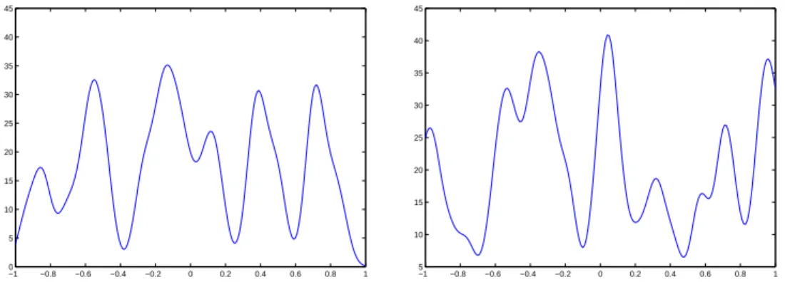
In this example, we see that taking T = 1 will create a large “bias” since the first of the two above integral will be equal to 0.5. In order to make both integrals negligible, one has to take T − 1 large compared to σ - say for instance T − 1 = 10σ, as illustrated in Figure 1.
−1 −0.8 −0.6 −0.4 −0.2 0 0.2 0.4 0.6 0.8 1 0 5 10 15 20 25 30 35 40 45 −1 −0.8 −0.6 −0.4 −0.2 0 0.2 0.4 0.6 0.8 1 5 10 15 20 25 30 35 40 45
Figure 1. Importance of the choice of the interval on which the Poisson points are sampled. Samples of a shot noise process on the interval [−1, 1] when: gσ is the
Gaussian kernel of width σ = 0.05, λ = 20 and β = 1. On the left: T = 1 and clearly there are some boundary effects. On the right, the simulation is obtained when taking T = 1.5 = 1 + 10σ. The boundary effects are no more noticeable.
2.3. Regularity. In this section, we focus on the sample path regularity of the shot noise process X given by (1). The process inherits regularity from the chosen kernel function as soon as sufficient integrability assumptions hold. We deal with two notions of regularity: a mean square one, which is valid for second order process and needs L2 assumptions and an almost sure one, which holds under uniform L1 assumptions. We refer to [25] who studies convergence of generalized shot noise series in
general Banach spaces.
Proposition 1. Let β ∈ L2(Ω) and g ∈ L1(R) ∩ L2(R). Assume that g ∈ C1(R) with g′ ∈ L1(R) ∩ L2(R) ∩ L∞(R). Then the shot noise process X given by (1) admits a mean square derivative.
Proof. Let us consider S(t, t′) = Cov (X(t), X(t′)) = λE(β2)R
Rg(t − s)g(t′− s)ν(ds), the covariance
function of the process X. According to Theorem 2.2.2 of [1] it is sufficient to remark that assumptions on g ensure that ∂t∂t∂2S′ exists and is finite at point (t, t) ∈ R2 with
(9) ∂ 2S ∂t∂t′(t, t) = λE(β 2)Z R g′(t − s)g′(t − s)ν(ds). Therefore for all t ∈ R the limit
X′(t) = lim
h→0
X(t + h) − X(t)
h ,
exists in L2(Ω) and the covariance function of the second-order process (X′(t))t∈Ris given by (t, t′) 7→
λE(β2)RRg′(t − s)g′(t′− s)ν(ds). ¤
This result only gives second order properties of the derivative and one can not deduce the law of X′. However, under uniform L1 assumptions, we can differentiate X under the sum as stated in the next proposition.
Proposition 2. Let β ∈ L1(Ω). Let g ∈ C1(R) ∩ L1(R). Assume that there exists ε > 0 such that Z R sup |t|≤ε|g ′(t − s)|ds < +∞,
then almost surely the series X(·) = X
i
βig(· − τi) converges uniformly on any compact set of R.
Moreover X is almost surely continuously differentiable on R with X′(t) =X
i
βig′(t − τi), ∀t ∈ R.
Proof. Let A > 0 and remark that for any s ∈ R and |t| ≤ A |g(t − s)| = ¯ ¯ ¯ ¯ Z t 0 g′(u − s)du + g(−s) ¯ ¯ ¯ ¯ ≤ Z A −A|g ′(s − u)|du + |g(−s)|,
such that by Fubini’s theorem and Assumption 1 Z R sup t∈[−A,A]|g(t − s)|ν(ds) ≤ 2A Z R|g ′(s)|ds + Z R|g(s)|ds < +∞.
Therefore, since β ∈ L1(Ω), the series X
i
βi sup
t∈[−A,A]|g(t − τi)| converges almost surely which means
that X
i
βig(· − τi) converges uniformly on [−A, A] almost surely. This implies that the sample
paths of X are almost surely continuous on R. Similarly, for all t0 ∈ R, almost surely the series
X
i
βig′(· − τi) converges uniformly on [t0− ε, t0 + ε] and therefore X is continuously differentiable
on [t0− ε, t0+ ε] with X′(t) =
X
i
βig′(t − τi) for all t ∈ [t0− ε, t0+ ε]. This concludes the proof
using the fact that R = ∪t0∈Q[t0− ε, t0+ ε]. ¤
Sufficient conditions to ensure both kinds of regularity are given in the following corollary. Corollary 1. Let β ∈ L2(Ω). Let g ∈ C2(R) such that g, g′, g′′ ∈ L1(R). Then X is almost surely
and mean square continuously differentiable on R with X′(t) =X
i
βig′(t − τi), ∀t ∈ R.
Proof. It is sufficient to check assumptions of Propositions 1 and 2. Note that g, g′ ∈ L1(R) imply that g ∈ L∞(R) ∩ L1(R) ⊂ L2(R). Similarly we also have g′ ∈ L2(R) ∩ L∞(R). Moreover since g′, g′′∈ L1(R), for any ε > 0 Z R sup |t|≤ε|g ′(t − s)|ds < +∞. ¤ Iterating this result one can obtain higher order smoothness properties. In particular it is straight-forward to obtain the following result for Gaussian kernels.
Example (Gaussian kernel): Let β ∈ L2(Ω), g(t) = g1(t) = √12πexp(−t2/2) and X given by
(1). Then, the process X is almost surely and mean square smooth on R. Moreover, for any n ∈ N, ∀t ∈ R, X(n)(t) =X i βig1(n)(t − τi) = X i βi(−1)nHn(t − τi)g1(t − τi) ,
3. Existence of a probability density for shot noise series
We focus in this section on the question of the existence of a probability density for a shot noise series. This question arises naturally when studying regularity in variation of the law [6] or level sets [19] of shot noise series. In particular the crossing theory for processes usually assumes the existence of a bounded density for the random vector (X(t), X′(t)) for t ∈ R. For sake of generality we consider here a Rd-valued shot noise process given on R by
(10) Y (t) =X
i
βih(t − τi),
where h : R 7→ Rd is a given (deterministic) measurable vectorial function in L1(R). In this setting
one can recover X given by (1) with d = 1 and h = g, or recover (X, X′)-if exists- with d = 2 and h = (g, g′).
The question of the existence of a probability density for the random vector Y (t) for some t ∈ R can be addressed from different points of view. One can exploit formula (10), where Y is written as a sum of random variables. It allows for instance to establish an integral equation to compute or approximate the density in some examples [22, 21, 15]. We adopt this point of view in the first part of this section to derive a sufficient condition for the existence of a density for Y . However it does not imply any continuity or boundedness of the distribution. Therefore, in the second part we deal with integrability property for the characteristic function, which implies both existence, continuity and boundedness of the density.
3.1. Sufficient condition for the existence of a density in the stationary case. In the following we assume that ν is the Lebesgue measure. Then, the Rd-valued process Y given by (10)
is stationary such that it is sufficient to study the law of the random vector Y (0). We introduce a truncated process in a similar way as in Section 2.2. We will use the same notations: let T > 0 and write Y (0) = YT(0) + RT(0) with YT(0) =
X
{i;|τi|≤T }
βih(−τi) independent from RT(0). Note that, as
in the one dimensional case
YT(0)=d
γT
X
i=1
βih(UT(i)),
where γT is a Poisson random variable of parameter λνT(R) = 2λT , {βi} are i.i.d. with common law
F , {UT(i)} are i.i.d. with uniform law on [−T, T ]. Here d
= stands for the equality in law and we recall the convention that
0
X
i=1
= 0.
Proposition 3. If there exists m ≥ 1 such that for any T > 0 large enough, conditionally on {γT = m}, the random variable YT(0) admits a density, then Y (0) admits a density.
Proof. Let T > 0 sufficiently large. First, let us remark that conditionally on {γT = m}, YT(0) = m
X
i=1
βih(UT(i)). Next, note that if a random vector V in Rd admits a density fV then, for UT with
uniform law on [−T, T ] and β with law F , independent of V , the random vector W = V + βh(UT)
admits w ∈ Rd7→ 2T1
R
R
RT
−TfV(w − zh(t))dtF (dz) for density. Therefore, by induction the
assump-tion implies that
n
X
i=1
βih(UT(i)) has a density, for any n ≥ m. Then, we follow the same lines as [3],
proof of Proposition A.2. Let A ⊂ Rdbe a Borel set with Lebesgue measure 0, since YT(0) and RT(0)
are independent
P(Y (0) ∈ A) = P(YT(0) + RT(0) ∈ A) =
Z
Rd
with µT the law of RT(0). But for any y ∈ Rd, P(YT(0) ∈ A − y) = P ÃγT X i=1 βih(UT(i)) ∈ A − y ! = +∞ X n=0 P ÃγT X i=1 βih(UT(i)) ∈ A − y | γT = n ! P(γT = n) = m−1X n=0 P Ã n X i=1 βih(UT(i)) ∈ A − y ! P(γT = n),
since A − y has Lebesgue measure 0 and
n
X
i=1
βi(h(UT(i))) has a density for any n ≥ m. Hence, for any
T > 0 large enough,
P(Y (0) ∈ A) ≤ P(γT ≤ m − 1).
Letting T → +∞ we conclude that P(Y (0) ∈ A) = 0 such that Y (0) admits a density. ¤ Let us remark that, under the assumptions of Proposition 3, considering YT(0) instead of Y (0) or
equivalently νT(ds) = 1I[−T,T ](s)ds instead of the Lebesgue measure, we would obtain that
condition-ally to {γT ≥ m} the random variable YT(0) admits a density. Let us emphasize that YT(0) does not
admit a density since P(YT(0) = 0) ≥ P(γT = 0) > 0.
Let us mention that Breton [6] gives a similar assumption for real-valued shot noise series in Proposition 2.1. In particular his Corollary 2.1. can be adapted in our multivalued setting.
Corollary 2. Let h : R 7→ Rd be an integrable function and β = 1 a.s. Let us define hd: Rd7→ Rd by
hd(x) = h(x1) + . . . + h(xd), for x = (x1, . . . , xd) ∈ Rd. If the hd image measure of the d-dimensional
Lebesgue measure is absolutely continuous with respect to the d-dimensional Lebesgue measure then the random vector Y (0), given by (10), admits a density.
Proof. Let A ⊂ Rda Borel set with Lebesgue measure 0 then assumptions ensure thatRRd1Ihd(x)∈Adx = 0. Therefore, for any T > 0, using notations of Proposition 3,
P Ã d X i=1 h(UT(i)) ∈ A ! = 1 (2T )d Z [−T,T ]d 1Ihd(x)∈Adx = 0. Hence d X i=1
h(UT(i)) admits a density and Proposition 3 gives the conclusion. ¤ Example (Gaussian kernel): let g(t) = √1
2πexp(−t
2/2), β = 1 a.s. and X given by (1). Let us
consider h = (g, g′) and h2 : (x1, x2) ∈ R2 7→ h(x1) + h(x2). The Jacobian of h2 is
J(h2)(x1, x2) = 1
2πP (x1, x2) exp(−(x
2
1+ x22)/2)
with P (x1, x2) = (1 + x1x2)(x1− x2). Hence, the h2 image measure of the 2-dimensional Lebesgue
measure is absolutely continuous with respect to the 2-dimensional Lebesgue measure. Then, for any t ∈ R, the random vector (X(t), X′(t)) is absolutely continuous with respect to the Lebesgue measure. Note that in particular this implies the existence of a density for X(t).
Most of results known on crossing theory for stationary processes (see for instance [2]) are based on the assumptions that for any t ∈ R, the random vector (X(t), X′(t)) admits a continuous bounded density. One way to get this assumption true is to check the integrability of the characteristic function of this vector.
3.2. Is the characteristic function integrable ? Existence and boundedness of a density. Let d ≥ 1 and consider a d-dimensional shot noise process Y (t) defined by Equation (10) with a kernel function h and impulse β = 1 a.s. When t ∈ R is fixed the characteristic function of Y (t) is defined by ψY (t)(u) = E(exp(iu · Y (t))), for u ∈ Rd. Let us remark that u · Y is a 1d shot noise
process with kernel u · h such that we get ψY (t)(u) = exp(λ
R
R(eiu·h(s)− 1) ν(ds)). Now, let us assume
that Z
Rdexp(−λ Z
R(1 − cos(u · h(s))) ν(ds))du < +∞.
This implies that ψY (t) belongs to L1(Rd) and thanks to Fourier inversion theorem, Y (t) has a
bounded continuous density (see for instance [13] p.482).
Examples: for d = 1 and ν(ds) = ds. We consider X the stationary shot noise process given by (1) and denote by ψ the characteristic function of X(t), t ∈ R, which does not depend on t.
• Power-law shot noise: if there exists A > 0 and α > 1/2 such that g(t) = 1/tα for t > A, then |ψ| is integrable. Actually, for any u 6= 0,
log |ψ(u)| ≤ −λ Z +∞ A (1 − cos(us −α)) ds = −λα1|u|1/α Z |u|A−α 0 1 − cos t t1+1/α dt.
Since the last integral has a finite positive limit as u goes to infinity, and since exp(−|u|1/α)
is integrable, this shows that |ψ| is integrable. Note that when g is causal i.e. g(t) = 0 for t < 0, one can define the shot noise process for A = 0 and α > 1. In this case, X(t) is a Levy stable random variable with stability index 1/α as proved in [21].
• Exponential kernel: if g(t) = e−t1I{t>0}, then |ψ| is integrable iff λ > 1. Actually, for |u| > 1, log |ψ(u)| = −λ Z +∞ 0 (1 − cos(ue −s)) ds = −λZ |u| 0 1 − cos(t) t dt = −λ ÃZ 1 0 1 − cos(t) t dt + log |u| − Z |u| 1 cos(t) t dt ! .
Since the last term in this sum has a finite limit as |u| goes to +∞, it proves that ψ(u) is integrable iff 1/|u|λ is, that is iff λ > 1.
• Compactly supported kernel: if g has compact support, then |ψ| is not integrable. Moreover X(t) does not admit a density. Actually, there exists A > 0 such that g(s) = 0 for |s| > A. Then RR(1 − cos(ug(s))) ds ≤ 2A, and thus |ψ(u)| ≥ exp(−2Aλ), which shows that it can not be integrable. Another way to see that |ψ| is not integrable in this case is to look at the probability of {X(t) = 0}. Indeed, X(t) is 0 as soon as there are no point of the Poisson process in the interval [−A, A], and such an event has a strictly positive probability. Thus P(X(t) = 0) > 0, which proves that X(t) doesn’t have a density, and consequently, |ψ| is not integrable.
It seems that the general picture is this: if g has “heavy tails”, then |ψ| is integrable, whereas when g(s) goes to 0 faster than exp(−|s|), then |ψ| is not integrable. A hint to understand this is the following idea: when g goes fast to 0, then P(|X(t)| ≤ ε) is “large” compared to ε, and thus the density of X(t), when it exists, is not bounded in a neighborhood of 0. And in particular, it implies that |ψ| is not integrable. All these statements are formalized in the following proposition.
Proposition 4. Let X be a stationary 1d shot noise process defined by (1) with kernel function g and ν(ds) = ds. Assume for sake of simplicity that β = 1 almost surely. Then:
(1) If g is such that there exist α > 1 and A > 0 such that ∀|s| > A, |g(s)| ≤ e−|s|α
, then ∃ε0 > 0
such that ∀0 < ε < ε0:
P(|X(t)| ≤ ε) ≥ 12e−2λTε where T
(2) If g is such that there exists A > 0 such that ∀|s| > A, |g(s)| ≤ e−|s| and if λ < 1/4 then ∃ε0 > 0 such that ∀0 < ε < ε0: P(|X(t)| ≤ ε) ≥ µ 1 − λ (1 − 2λ)2 ¶ e−2λTε where T ε is defined by Tε= − log ε.
This implies in both cases that P(|X(t)| ≤ ε)/ε goes to +∞ as ε goes to 0, and thus the density of X(t) -if it exists- is not bounded in a neighborhood of 0.
Proof. We start with the first case. Let ε > 0 and let Tε= (− log ε)1/α. Assume that ε is small enough
to have Tε> A. We have by definition X(t)= X(0)d =d
X i g(τi). If we denote XTε(0) = X |τi|≤Tε g(τi) and RTε(0) = X |τi|>Tε
g(τi), then XTε(0) and RTε(0) are independent and X(0) = XTε(0) + RTε(0). We also have: P(|X(0)| ≤ ε) ≥ P(|XTε(0)| = 0 and |RTε(0)| ≤ ε) = P(|XTε(0)| = 0) × P(|RTε(0)| ≤ ε). Now on the one hand we have: P(|XTε(0)| = 0) ≥ P( there are no τi in [−Tε, Tε]) = e−2λTε. On the other hand, the first moments of the random variable RTε(0) are given by: E(RTε(0)) =
λR|s|>T+∞
εg(s) ds and Var(RTε(0)) = λ R+∞
|s|>Tεg
2(s) ds. Now, we use the following inequality on the tail
ofR e−sα : ∀T > 0, e−Tα = Z +∞ T αsα−1e−sαds ≥ αTα−1 Z +∞ T e−sαds. Thus, we obtain bounds for the tail of Rg and of Rg2 :
Z +∞ T e−sαds ≤ e−T α αTα−1 and Z +∞ T ¡ e−sα¢2 ds ≤ e−2T α 2αTα−1.
Back to the moments of RTε(0), since Tε= (− log ε)
1/α we have: |E(RTε(0))| ≤ 2λε αTεα−1 and Var(RTε(0)) ≤ λε2 αTεα−1 .
We can take ε small enough in such a way that we can assume that |E(RTε(0))| < ε. Then, using Chebyshev’s inequality, we have
P(|RTε(0)| ≤ ε) = P(−ε − E(RTε(0)) ≤ RTε(0) − E(RTε(0)) ≤ ε − E(RTε(0))) ≥ 1 − P(|RTε(0) − E(RTε(0))| ≥ ε − |E(RTε(0))|) ≥ 1 − Var(RTε(0)) (ε − |E(RTε(0))|)2 ≥ 1 − λ αTεα−1(1 − 2λ/αTεα−1)2 , which is larger than 1/2 for Tε large enough (i.e. for ε small enough).
For the second case, we can make exactly the same computations by setting α = 1, and get P(|RTε(0)| ≤ ε) ≥ 1 − λ/(1 − 2λ)2, which is > 0 when λ < 1/4. ¤ Example (Gaussian kernel): Let g(t) = √1
2πexp(−t
2/2), ν(ds) = ds, β = 1 a.s. and X given
by (1). Then, for any t ∈ R, the random variable X(t) admits a density that is not bounded in a neighborhood of 0.
Such a feature is particularly bothersome when considering crossings of these processes since most of known results are based on the existence of bounded density for each marginal of the process. However such a behavior is extremely linked to the number of points of the Poisson process {τi} that
are thrown in the interval of study. The density -if it exists- will be more regular as this number increases. This can be settled considering the integrability of the characteristic function conditionally on a certain number of points in the interval. Then, the main tool is the classical stationary phase estimate for oscillatory integrals (see [29] for example). We will moreover need such results in the framework of two variables (u, v), when studying crossing functions.
Proposition 5 (Stationary phase estimate for oscillatory integrals). Let a < b and let ϕ be a function of class C2 defined on [a, b]. Assume that ϕ′ and ϕ′′cannot simultaneously vanish on [a, b] and denote m = min
s∈[a,b]
p
ϕ′(s)2+ ϕ′′(s)2 > 0. Let us also assume that n
0 = #{s ∈ [a, b] s. t. ϕ′′(s) = 0} < +∞. Then ∀u ∈ R s.t. |u| > m1 , ¯ ¯ ¯ ¯ Z b a eiuϕ(s)ds ¯ ¯ ¯ ¯ ≤ 8 √ 2(2n0+ 1) p m|u| .
Now, let ϕ1 and ϕ2 be two functions of class C3 defined on [a, b]. Assume that the derivatives
of these functions are linearly independent, in the sense that for all s ∈ [a, b], the matrix Φ(s) = µ
ϕ′1(s) ϕ′2(s) ϕ′′
1(s) ϕ′′2(s)
is invertible. Denote m = min
s∈[a,b] k Φ(s)
−1 k−1> 0, where k · k is the matricial
norm induced by the Euclidean one. Assume moreover that there exists n0 < +∞ such that #{s ∈
[a, b] s.t. det(Φ′(s)) = 0} ≤ n0, where Φ′(s) =
µ ϕ′′1(s) ϕ′′2(s) ϕ(3)1 (s) ϕ(3)2 (s) ¶ . Then ∀(u, v) ∈ R2 s.t. pu2+ v2> 1 m, ¯ ¯ ¯ ¯ Z b a eiuϕ1(s)+ivϕ2(s)ds ¯ ¯ ¯ ¯ ≤ 8√2(2n0+ 3) p m√u2+ v2.
Proof. For the first part of the proposition, by assumption, [a, b] is the union of the three compact sets
©
s ∈ [a, b]; |ϕ′′| ≥ m/2ª,©s ∈ [a, b]; |ϕ′| ≥ m/2 and ϕ′′≥ 0ª and ©s ∈ [a, b]; |ϕ′| ≥ m/2 and ϕ′′≤ 0ª. Therefore there exists 1 ≤ n ≤ 2n0+ 1 and a subdivision (ai)0≤i≤n of [a, b] such that [ai−1, ai] is
included in one of the previous subsets for any 1 ≤ i ≤ n. If [ai−1, ai] ⊂ {s ∈ [a, b]; |ϕ′′(s)| ≥ m/2},
according to Proposition 2 p.332 of [29] ¯ ¯ ¯ ¯ ¯ Z ai ai−1 eiuϕ(s)ds ¯ ¯ ¯ ¯ ¯= ¯ ¯ ¯ ¯ ¯ Z ai ai−1 eiu(m/2)(2ϕ(s)/m)ds ¯ ¯ ¯ ¯ ¯≤ 8 √ 2 p m|u|; otherwise, ¯ ¯ ¯ ¯ ¯ Z ai ai−1 eiuϕ(s)ds ¯ ¯ ¯ ¯ ¯≤ 6 m|u| The result follows from summing up these n integrals.
For the second part of the proposition, we use polar coordinates, and write (u, v) = (r cos θ, r sin θ). For θ ∈ [0, 2π), let ϕθ be the function defined on [a, b] by ϕθ(s) = ϕ1(s) cos θ + ϕ2(s) sin θ. Then
µ ϕ′θ(s) ϕ′′ θ(s) ¶ = Φ(s) µ cos θ sin θ ¶ , and thus 1 =k Φ(s)−1 µ ϕ′θ(s) ϕ′′ θ(s) 
k. This implies that for all s ∈ [a, b], p
ϕ′θ(s)2+ ϕ′′
θ(s)2 ≥ 1/ k Φ(s)−1 k≥ m. Moreover, thanks to Rolle’s Theorem, the number of
points s ∈ [a, b] such that ϕ′′
θ(s) = 0 is bounded by one plus the number of s ∈ [a, b] such that
ϕ′′1(s)ϕ′′′2(s) − ϕ′′′1(s)ϕ′′2(s) = 0, that is by 1 + n0. Thus, we can apply the result of the first part
of the proposition to each function ϕθ and the obtained bound will depend only on m, n0 and
r =√u2+ v2. ¤
Proposition 6. Let X be a stationary 1d shot noise process defined by (1) with kernel function g ∈ L1(R) and ν(ds) = ds. Assume for sake of simplicity that β = 1 almost surely. Let T > 0 and γT = #{i; τi ∈ [−T, T ]}. Let a < b and assume that g is a function of class C2 on [−T + a, T + b]
such that m = min s∈[−T +a,T +b] p g′(s)2+ g′′(s)2 > 0 and n 0= #{s ∈ [−T + a, T + b] s. t. g′′(s) = 0} < +∞.
Then, conditionally on {γT ≥ k0} with k0≥ 3, for all t ∈ [a, b], the law of X(t) admits a continuous
Proof. Actually, we will prove that conditionally on {γT ≥ k0}, the law of the truncated process
XT(t) =
X
|τi|≤T
g(t − τi) admits a continuous bounded density for t ∈ [a, b]. The result will follow,
using the fact that X(t) = XT(t) + RT(t), with RT(t) independent from XT(t), as given by (8).
Therefore let us denote ψTt,k0 the characteristic function of XT(t) conditionally on {γT ≥ k0}. Then,
for all u ∈ R, we get
ψt,kT 0(u) = 1 P(γT ≥ k0) X k≥k0 E³eiuXT(t)|γ T = k ´ P(γT = k) = 1 P(γT ≥ k0) X k≥k0 µ 1 2T Z T −T eiug(t−s)ds ¶k e−2λT(2λT ) k k! Therefore, ¯ ¯ψT t,k0(u) ¯ ¯ ≤ (2T)−k0 ¯ ¯ ¯ ¯ Z T +t −T +t eiug(s)ds ¯ ¯ ¯ ¯ k0 .
Hence, using Proposition 5 on [−T + t, T + t] ⊂ [−T + a, T + b], one can find C a positive constant that depends on T , k0, λ, m and n0 such that for any |u| > 1/m
¯ ¯ψT t,k0(u) ¯ ¯ ≤ C|u|−k0/2. Then ψT
t,k0 is integrable on R, since k0 ≥ 3, and thanks to Fourier inverse Theorem it is the
charac-teristic function of a bounded continuous density. ¤
4. Crossings
The goal of this section is to investigate crossings for smooth shot noise processes. This is a very different situation from the one studied in [22, 4, 17] where shot noise processes are non differentiable. However crossings of smooth processes have been extensively studied especially in the Gaussian processes realm (see [2] for instance). Then, most of known results are based on assumptions on density probabilities, which are not well-adapted in our setting, as seen in the previous section. In the next subsection, we revisit these results with a more adapted point of view based on characteristic functions.
4.1. General formula. When X is an almost surely continuously differentiable process on R, we can consider its multiplicity function on an interval [a, b] defined by
(11) ∀α ∈ R, NX(α, [a, b]) = #{t ∈ [a, b]; X(t) = α}.
This defines a positive random process taking integer values. Let briefly recall some points of “vo-cabulary”. For a given level α ∈ R, a point t ∈ [a, b] such that X(t) = α is called “crossing” of the level α. Then NX(α, [a, b]) counts the number of crossings of the level α in the interval [a, b]. Now we
have to distinguish three different types of crossings (see for instance [9]): the up-crossings are points for which X(t) = α and X′(t) > 0, the down-crossings are points for which X(t) = α and X′(t) < 0 and the tangencies are points for which X(t) = α and X′(t) = 0. The following proposition gives a simple criterion which ensures that the number of tangencies is 0 almost surely.
Proposition 7. Let a, b ∈ R with a ≤ b. Let X be a real valued random process almost surely C2 on [a, b]. Let us assume that there exists φ ∈ L1(R) and C
a,b> 0 such that
∀t ∈ [a, b], ¯¯¯E³eiuX(t)´¯¯¯ ≤ Ca,bφ(u).
Then,
Proof. Let M > 0 and let denote AM the event corresponding to max t∈[a,b]|X ′(t)| ≤ M and max t∈[a,b] ¯ ¯X′′(t)¯¯ ≤ M such that P ¡∃t ∈ [a, b], X(t) = α, X′(t) = 0¢= lim M →+∞P ¡∃t ∈ [a, b], X(t) = α, X ′(t) = 0, A M¢.
Note that on AM, for t, s ∈ [a, b], we have by the mean value theorem
|X(t) − X(s)| ≤ M|t − s| and |X′(t) − X′(s)| ≤ M|t − s|.
Let us assume that there exists t ∈ [a, b] such that X(t) = α and X′(t) = 0. Then for any n ∈ N there exists kn∈ [2na, 2nb] ∩ Z such that |t − 2−nkn| ≤ 2−nwith, by Taylor formula,
|X(2−nkn) − α| ≤ 2−2nM and |X′(2−nkn)| ≤ 2−nM.
Therefore, let us denote
Bn= ∪
kn∈[2na,2nb]∩Z
©
|X(2−nkn) − α| ≤ 2−2nM and |X′(2−nkn)| ≤ 2−nMª.
Since (Bn∩ AM)n∈N is a decreasing sequence we get
P ¡∃t ∈ [a, b]; X(t) = α, X′(t) = 0, A M
¢
≤ lim
n→+∞P(Bn∩ AM).
But, according to assumption, for any n ∈ N the random variable X(2−nkn) admits a uniformly
bounded density function. Therefore, there exists ca,b such that
P ¡|X(2−nk
n) − α| ≤ 2−2nM, |X′(2−nkn)| ≤ 2−nM¢≤ ca,b2−2nM.
Hence
P(Bn∩ AM) ≤ (b − a + 1)ca,b2−nM,
which yields the result. ¤
In particular, assumptions of Proposition 7 allow us to use Kac’s counting formula (see Lemma 3.1 [2]), which we recall in the following proposition.
Proposition 8 (Kac’s counting formula). Let a, b ∈ R with a < b. Let X be a real valued random process defined on R almost surely continuously differentiable on [a, b]. Let α ∈ R. Assume that (12) P(∃t ∈ [a, b] s.t. X(t) = α and X′(t) = 0) = 0 and P(X(a) = α) = P(X(b) = α) = 0.
Then, almost surely
NX(α, [a, b]) = lim δ→0 1 2δ Z b a 1I|X(t)−α|<δ|X′(t)|dt.
To study crossings, one can also use the co-area formula which is valid in the framework of bounded variations functions (see for instance [12]), but we won’t need here such a general framework. When X is an almost surely continuously differentiable process on [a, b], for any bounded and continuous function h on R, we have: (13) Z b a h(X(t))|X ′(t)| dt =Z R h(α)NX(α, [a, b]) dα a.s.
In particular when h = 1 this shows that α 7→ NX(α, [a, b]) is integrable on R and
R
RNX(α, [a, b]) dα =
Rb
a|X′(t)| dt is the total variation of X on [a, b].
Let us also recall that when there are no tangencies of X′ for the zero-level, then the number
of local extrema for X is given by NX′(0, [a, b]), which corresponds to the sum of the number of local minima (up zero-crossings of X′) and of local maxima (down zero-crossings of X′). Moreover,
according to Rolle’s theorem, whatever the level α is, NX(α, [a, b]) ≤ NX′(0, [a, b]) + 1 a.s.
Dealing with random processes one may be more interested in the mean number of crossings. We will denote by CX(α, [a, b]) the mean number of crossings of the level α by the process X in [a, b]:
Let us emphasize that this function is no more with integer values and can be continuous with respect to α. When moreover X is a stationary process, by the additivity of means, we get CX(α, [a, b]) =
(b − a)CX(α, [0, 1]) for α ∈ R. In this case CX(α, [0, 1]) corresponds to the mean number of crossings
of the level α per unit length. Let us also recall that when X is a strictly stationary ergodic process, the ergodic theorem states that (2T )−1NX(α, [−T, T ]) −→
T →+∞CX(α, [0, 1]) a.s. (see [9] for instance).
A straightforward result can be derived from the co-area formula (13).
Proposition 9. Let a, b ∈ R with a < b. Let X be an almost surely and mean square continu-ously differentiable process on [a, b]. Then α 7→ CX(α, [a, b]) ∈ L1(R). Moreover, for any bounded
continuous function h: (15) Z b a E(h(X(t))|X ′(t)|)dt =Z R h(α)CX(α, [a, b]) dα.
Proof. Taking the expected values in (13) for h = 1 on the interval [a, b] we get by Fubini’s theorem
that Z b a E(|X ′(t)|)dt =Z R CX(α, [a, b]) dα.
Since t 7→ E(|X′(t)|) is continuous on [a, b] by mean square continuity of X′, the total variation of X
on [a, b] has finite expectation, which concludes the proof. ¤
Let us emphasize that this result implies in particular that CX(α, [a, b]) < +∞ for almost every
level α ∈ R but one cannot conclude for a fixed given level.
One should expect to have a similar formula for CX than the Kac’s formula obtain for NX.
However, when X is a process satisfying the assumptions of Proposition 8, Kac’s formula only gives an upper bound on CX(α, [a, b]), according to Fatou’s Lemma:
CX(α, [a, b]) ≤ lim inf δ→0 1 2δ Z b a E ¡1I|X(t)−α|<δ|X′(t)|¢dt.
This upper bound is not very tractable without assumptions on the existence of a bounded joint density for the law of (X(t), X′(t)). As far as shot noise processes are concerned, one can exploit the infinite divisibility property by considering the mean crossing function of the sum of independent processes. The next proposition gives an upper bound in this setting. Another application of this proposition will be seen in Section 6 where we will decompose a shot noise process into the sum of two independent processes (for which crossings are easy to compute) by partitioning the set of points of the Poisson process.
Proposition 10 (Crossings of a sum of independent processes). Let a, b ∈ R with a < b. Let n ≥ 2 and Xj be independent real-valued processes almost surely and mean square two times continuously
differentiable on [a, b] for 1 ≤ j ≤ n. Assume that there exist constants Cj and probability measures
dµj on R such that if dPXj(t) denotes the probability measure of Xj(t), then ∀t ∈ [a, b], dPXj(t) ≤ Cjdµj, for 1 ≤ j ≤ n. Let X be the process obtained by X =
n
X
j=1
Xj and assume that X satisfies (12) for α ∈ R. Then
(16) CX(α, [a, b]) ≤ n X j=1 Y i6=j Ci (CX′ j(0, [a, b]) + 1).
Moreover, in the case where all the Xj are stationary on R:
CX(α, [a, b]) ≤ n X j=1 CX′ j(0, [a, b]).
Proof. We first need an elementary result. Let f be a C1 function on [a, b], then for all δ > 0, and for all x ∈ R, we have:
(17) 1
2δ Z b
a
1I|f(t)−x|≤δ|f′(t)| dt ≤ Nf′(0, [a, b]) + 1.
This result (that can be found as an exercise at the end of Chapter 3 of [2]) can be proved this way: let a1 < . . . < an denote the points at which f′(t) = 0 in [a, b]. On each interval [a, a1], [a1, a2], . . . ,
[an, b], f is monotonic and thus
Rai+1
ai 1I|f(t)−x|≤δ|f
′(t)| dt ≤ 2δ. Summing up these integrals, we have
the announced result.
For the process X, since it satisfies the conditions of Kac’s formula (12), by Proposition 8 and Fatou’s Lemma,
CX(α, [a, b]) ≤ lim inf δ→0 1 2δ Z b a E(1I|X(t)−α|≤δ|X′(t)|) dt.
Now, for each δ > 0, we have E(1I|X(t)−α|≤δ|X′(t)|) ≤
n
X
j=1
E(1I|X1(t)+...+Xn(t)−α|≤δ|Xj′(t)|). Then,
thanks to the independence of X1, . . . , Xn and to the bound on the laws of Xj(t), we get:
Z b a E(1I|X1(t)+...+Xn(t)−α|≤δ|X′ 1(t)|) dt = Z b a Z Rn−1 E(1I|X1(t)+x2+...+xn−α|≤δ|X′ 1(t)| | X2(t) = x2, . . . , Xn(t) = xn) dPX2(t)(x2) . . . dPXn(t)(xn) dt ≤ n Y j=2 Cj Z Rn−1 Z b a E(1I|X1(t)+x2+...+xn−α|≤δ|X1′(t)|) dt dµ2(x2) . . . dµn(xn).
Now, (17) holds almost surely for X1, taking expectation we get
1 2δ
Z b a
E(1I|X1(t)+x2+...+xn−α|≤δ|X1′(t)|) dt ≤ CX1′(0, [a, b]) + 1.
Using the fact the dµj are probability measures we get
1 2δ Z b a E(1I|X1(t)+...+Xn(t)−α|≤δ|X1′(t)|) dt ≤ n Y j=2 Cj (CX′ 1(0, [a, b]) + 1).
We obtain similar bounds for the other terms. Since this holds for all δ > 0, we have the bound (16) on the expected number of crossings of the level α by the process X.
When the Xj are stationary, things become simpler: we can take Cj = 1 for any 1 ≤ j ≤ n, and also
by stationarity we have that for all p ≥ 1 integer: CX(α, [a, b + p(b − a)]) = (p + 1)CX(α, [a, b]). Now
using (16) for all p, then dividing by (p + 1), we have that for all p: CX(α, [a, b]) ≤ n X j=1 CX′ j(0, [a, b]) + n
p + 1. Finally, letting p goes to infinity, we have the result. ¤
As previously seen, taking the expectation in Kac’s formula only allows us to get an upper bound for CX. However, under stronger assumptions, one can justify the interversion of the limit and the
expectation. This is known as Rice’s formula. We recall it here under original assumptions on the characteristic functions of the process, which are more tractable than densities, in the setting of shot noise processes.
Proposition 11 (Rice’s Formula). Let a, b ∈ R with a ≤ b. Let X be a real valued random process almost surely continuously differentiable on [a, b]. Let us denote ψt,ε, respectively ψt,0 := ψt, the
ε > 0. Assume that for all t ∈ [a, b] and ε sufficiently small, and for all 0 ≤ k ≤ 3, the partial derivatives ∂v∂kkψt,ε(u, v) exist and satisfy
(18) ¯ ¯ ¯ ¯ ∂ k ∂vkψt,ε(u, v) ¯ ¯ ¯ ¯ ≤ C(1 + p u2+ v2)−l,
for l > 2 and C a positive constant. Then, the crossings mean number function α 7→ CX(α, [a, b]) is
continuous on R and given by
(19) CX(α, [a, b]) = Z b a Z R|z|p t(α, z) dz dt < +∞, where pt(α, z) = 4π12 ˇ b
ψt(α, z) is the joint distribution density of (X(t), X′(t)).
Proof. It is enough to check assumptions i)–iii) of Theorem 2 of [19] p.262. Assumptions for k = 0 ensure that ψt,ε∈ L1(R2), respectively ψt∈ L1(R2), such that (X(t), (X(t+ε)−X(t))/ε), respectively
(X(t), X′(t)), admits pt,ε= 4π12 ˇ d ψt,ε, respectively pt= 4π12 ˇ b ψt, as density.
i) pt,ε(x, z) is continuous in (t, x) for each z, ε, according to Lebesgue’s dominated convergence
theorem using the fact that X is almost surely continuous on R.
ii) Since X is almost surely continuously differentiable on R we clearly have for any (u, v) ∈ R2, ψt,ε(u, v) → ψt(u, v) as ε → 0. Then by Lebesgue’s dominated convergence theorem pt,ε(x, z) →
pt(x, z) as ε → 0, uniformly in (t, x) for each z ∈ R.
iii) For any z 6= 0, integrating by parts we get pt,ε(x, z) = i 4π2z3 Z R2 e−ixu−izv ∂ 3 ∂v3ψt,ε(u, v)dudv,
such that pt,ε(x, z) ≤ Ch(z) for all t, ε, x with h(z) = (1 + |z|3)−1 satisfying
R
R|z|h(z)dz < +∞ and
C a positive constant. ¤
Let us mention that Rice’s formula (19) can be obtained under weaker assumption when considering X strictly stationary and mean square differentiable on [a, b]. Actually, according to Theorem 2 iii) of [14], if P(X′(0) = 0) = 0 then the law of X(0) has a density denoted by fX(0)(x)dx, and Rice’s
formula (19) holds for fX(0)(x)dx-almost every α ∈ R. If the joint distribution density does not exist
the integral on R is replaced by fX(0)(α)E (|X′(0)| | X(0) = α).
However, let us emphasize that Proposition 11 states also that the crossings mean number function α 7→ CX(α, [a, b]), which was already known to be integrable, is also continuous on R.
We have not been able to obtain this property by a different way with weaker assumptions. We use it to state the next theorem concerning shot noise processes.
Theorem 1. Let X be a stationary 1d shot noise process defined by (1) with kernel function g and ν(ds) = ds. Assume for sake of simplicity that β = 1 almost surely. Let us assume that g is a function of class C4 on R with g, g′, g′′ ∈ L1(R). Let T > 0, a ≤ b, and assume that for all s ∈ [−T + a, T + b], the matrices Φ(s) = µ g′(s) g′′(s) g′′(s) g(3)(s) ¶ and Φ′(s) = µ g′′(s) g(3)(s) g(3)(s) g(4)(s) ¶ are invertible. Let γT = #{i; τi ∈ [−T, T ]}. Then, conditionally on {γT ≥ k0} with k0 ≥ 8, the crossings
mean number function α 7→ E (NX(α, [a, b])|γT ≥ k0) is continuous on R.
Proof. Let t ∈ [a, b]. We write X(t) = XT(t) + RT(t) as given by (8). Let us write for ε small enough
ψt,ε,k0 = ψ T t,ε,k0ψ RT t,ε with ψt,ε,k0, respectively ψ T
t,ε,k0, the characteristic function of (X(t), (X(t+ε)−X(t))/ε), respectively
(XT(t), (XT(t + ε) − XT(t))/ε), conditionally on {γT ≥ k0}. Note that, RT is independent from γT
such that ψRT
t,ε is just the characteristic function of (RT(t), (RT(t + ε) − RT(t))/ε). According to
Rice’s formula the result will follow from (18). By Leibnitz formula, for 0 ≤ k ≤ 3, one has
(20) ∂ k ∂vkψt,ε,k0(u, v) = k X l=0 µ k l ¶ ∂l ∂vlψ T t,ε,k0(u, v) ∂k−l ∂vk−lψ RT t,ε (u, v).
On the one hand ¯ ¯ ¯ ¯ ∂ k−l ∂vk−lψ RT t,ε (u, v) ¯ ¯ ¯ ¯ ≤E ï¯ ¯ ¯RT(t + ε) − Rε T(t) ¯ ¯ ¯ ¯ k−l! , with ¯ ¯ ¯ ¯ RT(t + ε) − RT(t) ε ¯ ¯ ¯ ¯ ≤ X |τi|>T |gε(t − τi)| for gε(s) = 1 ε Z ε 0 g′(s + x)dx.
Let us remark that since g′, g′′ ∈ L1(R) one has g, g′ ∈ L∞(R). Then for any ε > 0, gε ∈ L∞(R) ∩
L1(R) with kgεk∞≤ kg′k∞ and kgεk1 ≤ kg′k1. Then using (7), one can find c > 0 such that for all
0 ≤ k ≤ 3, with (k − 1)+= max(0, k − 1), (21) ¯ ¯ ¯ ¯ ∂k ∂vkψ RT t,ε(u, v) ¯ ¯ ¯ ¯ ≤ c max(1, kg′k∞)(k−1)+max(1, λkg′k1)k.
On the other hand,
P(γT ≥ k0)ψt,ε,kT 0(u, v) = X k≥k0 E³eiuXT(t)+iv(XT(t+ε)−XT(t))/ε|γ T = k ´ P(γT = k) = X k≥k0 χTt,ε(u, v)kP(γT = k)
where χTt,ε(u, v) = (2T )−1R−T +tT +t eiug(s)+ivgε(s)ds, is the characteristic function of (g(t−U
T), gε(t−UT)),
with UT a uniform random variable on [−T, T ]. It follows that
¯ ¯χT
t,ε(u, v)
¯
¯ ≤ 1, so that one can find c > 0 such that for all 0 ≤ k ≤ 3,
¯ ¯ ¯ ¯ ∂ k ∂vkψ T t,ε,k0(u, v) ¯ ¯ ¯ ¯ ≤ c max(1, kg′k∞)(k−1)+max(1, λkg′k1)k P(γT ≥ k0− k) P(γT ≥ k0) ¯ ¯χT t,ε(u, v) ¯ ¯k0−k . This, together with (21) and (20), implies that one can find c > 0 such that for all 0 ≤ k ≤ 3, (22) ¯ ¯ ¯ ¯ ∂k ∂vkψt,ε,k0(u, v) ¯ ¯ ¯ ¯ ≤ c max(1, kg′k∞)(k−1)+max(1, λkg′k1)kP(γT ≥ k0− k) P(γT ≥ k0) ¯ ¯χT t,ε(u, v) ¯ ¯k0−k . Moreover, let Φε(s) = µ g′(s) g′ ε(s) g′′(s) gε′′(s) ¶ and Φ′ ε(s) = µ g′′(s) g′′ ε(s) g(3)(s) g(3)ε (s) 
. Then detΦε(s) converges
to detΦ(s) as ε → 0, uniformly in s ∈ [−T − a, T + b]. The assumption on Φ ensures that one can find ε0 such that for ε ≤ ε0, the matrix Φε(s) is invertible for all s ∈ [−T − a, T + b]. The same holds
true for Φ′ε(s). Denote m = min
s∈[−T −a,T +b],ε≤ε0 k Φ
ε(s)−1 k−1> 0, where k · k is the matricial norm
induced by the Euclidean one. According to Proposition 5 with n0 = 0,
∀(u, v) ∈ R2 s. t. pu2+ v2 > 1 m, ¯ ¯χT t,ε(u, v) ¯ ¯ = (2T )−1 ¯ ¯ ¯ ¯ Z T +t −T +t eiug(s)+ivgε(s)ds ¯ ¯ ¯ ¯ ≤ 24 √ 2 p m√u2+ v2.
Therefore, one can find a constant ck0 > 0 such that, for all 0 ≤ k ≤ 3, ¯ ¯ ¯∂v∂kkψt,ε,kT 0(u, v) ¯ ¯ ¯ is less than ck0(2T )−k0 +3max(1, kg′k ∞)(k−1)+max(1, λkg′k1)kP(γT ≥ k0− k) P(γT ≥ k0) ³ 1 +pu2+ v2´−(k0−3)/2,
with (k0− 3)/2 > 2 when k0> 7 so that (18) holds, which concludes the proof. ¤
As previously seen, the classical Rice’s formula for the mean crossings number function, when it holds, involves the joint probability density of (X(t), X′(t)). Such a formula is not tractable in our context where the existence of a density is even a question in itself. Considering the crossings mean number as an integrable function, it is natural to consider its Fourier transform as we do in the next section.
4.2. Fourier transform of crossings mean number. In the following proposition we obtain a closed formula for the Fourier transform of the crossings mean number function, which only involves characteristic functions of the process. This can be helpful, when considering shot noise processes, whose characteristic functions are well-known.
Proposition 12. Let a, b ∈ R with a < b. Let X be an almost surely and mean square continuously differentiable process on [a, b]. Then α 7→ CX(α, [a, b]) ∈ L1(R) and its Fourier transform u 7→
d
CX(u, [a, b]) is given by
(23) dCX(u, [a, b]) =
Z b a
E³eiuX(t)
|X′(t)|´dt.
Moreover, if ψt denotes the joint characteristic function of (X(t), X′(t)), then dCX(u, [a, b]) can be
computed by d CX(u, [a, b]) = − 1 π Z b a Z +∞ 0 1 v µ ∂ψt ∂v (u, v) − ∂ψt ∂v (u, −v) ¶ dv dt = −1π Z b a Z +∞ 0 1
v2 (ψt(u, v) + ψt(u, −v) − 2ψt(u, 0)) dv dt.
Proof. According to Proposition 9 we can choose h in Equation (15) of the form h(x) = exp(iux) for any u real. This shows that bC(u, [a, b]) =RabE ¡eiuX(t)|X′(t)|¢dt. Let us now identify the right-hand
term. Let µt(dx, dy) denote the distribution of (X(t), X′(t)). Then the joint characteristic function
ψt(u, v) of (X(t), X′(t)) is ψt(u, v) = E ¡ exp(iuX(t) + ivX′(t))¢= Z R2 eiux+ivyµt(dx, dy).
Since the random vector (X(t), X′(t)) has moment of order two, then ψtis twice continuously
differ-entiable on R2. Now, let us consider the integral IA = Z A 0 1 v µ ∂ψt ∂v (u, v) − ∂ψt ∂v (u, −v) ¶ dv = Z A v=0 Z x,y∈R2
iyeiux+ivy− iyeiux−ivy
v µt(dx, dy) dv = −2 Z A v=0 Z R2 yeiuxsin(vy) v µt(dx, dy) dv = −2 Z R2 yeiux Z Ay v=0 sin(v) v dvµt(dx, dy)
The order of integration has been reversed thanks to Fubini’s Theorem ( |yeiux sin(vy)v | ≤ y2 which
is integrable on [0, A] × R2 with respect to dv × µ
t(dx, dy), since X′(t) is a second order random
variable). As A goes to +∞, thenRv=0Ay sin(v)
v dv goes to π2sign(y), and moreover for all A, x and y,
we have |yeiuxRAy v=0
sin(v)
v dv| ≤ 3|y|, thus by Lebesgue’s dominated convergence theorem, the limit of
−π1IA exists as A goes to infinity and its value is:
lim A→+∞− 1 π Z A 0 1 v µ ∂ψt ∂v(u, v) − ∂ψt ∂v (u, −v) ¶ dv = Z R2|y|e iuxµ t(dx, dy) = E ³ eiuX(t)|X′(t)|´.
The second expression in the proposition is simply obtained by integration by parts in the above
formula. ¤
It is then natural to invert the Fourier transform to get an almost everywhere expression for CX(α, [a, b]) itself.
Proposition 13. Let a, b ∈ R with a ≤ b. Let X be a real valued random process almost surely continuously differentiable on [a, b]. Let us denote ψt the characteristic function of (X(t), X′(t)), for
t ∈ [a, b]. Assume that for all t ∈ [a, b], for 1 ≤ k ≤ 2, the partial derivatives ∂v∂kkψt(u, v) exist and satisfy (24) ¯ ¯ ¯ ¯ ∂ k ∂vkψt(u, v) ¯ ¯ ¯ ¯ ≤ C(1 + p u2+ v2)−l,
for l > 1 and C a positive constant. Then dCX(u, [a, b]) ∈ L1(R) and for almost every α ∈ R (25) CX(α, [a, b]) = − 1 2π2 Z b a Z R Z +∞ 0 e−iuα v µ ∂ψt ∂v(u, v) − ∂ψt ∂v(u, −v) ¶ dv du dt. Proof. Let u ∈ R and t ∈ [a, b], according to Proposition 12 one has
E³eiuX(t)|X′(t)|´ = −1 π Z +∞ 0 1 v µ ∂ψt ∂v (u, v) − ∂ψt ∂v (u, −v) ¶ dv It is sufficient to remark that integrating by parts, for any ε ∈ (0, 1),
Z 1 ε 1 v µ ∂ψt ∂v (u, v) − ∂ψt ∂v (u, −v) ¶ dv = − ln(ε) µ ∂ψt ∂v (u, ε) − ∂ψt ∂v(u, −ε) ¶ − Z 1 ε ln(v) µ ∂2ψt ∂v2 (u, v) − ∂2ψt ∂v2 (u, −v) ¶ dv. Therefore, as ε goes to zero, one gets
(26) Z 1 0 1 v µ ∂ψt ∂v(u, v) − ∂ψt ∂v(u, −v) ¶ dv = − Z 1 0 ln(v) µ ∂2ψ t ∂v2 (u, v) − ∂2ψ t ∂v2 (u, −v) ¶ dv. Then, according to (24) for k = 2,
¯ ¯ ¯ ¯ Z 1 0 1 v µ ∂ψt ∂v(u, v) − ∂ψt ∂v(u, −v) ¶ dv ¯ ¯ ¯ ¯ ≤ 2C(1 + |u|)−l. On the other hand, according to (24) for k = 1,
¯ ¯ ¯ ¯ Z +∞ 1 1 v µ ∂ψt ∂v (u, v) − ∂ψt ∂v (u, −v) ¶ dv ¯ ¯ ¯ ¯ ≤ C′(1 + |u|)−lln(2 + |u|).
Then dCX(u, [a, b]) ∈ L1(R) and its inverse Fourier transform given by (25) is equal to CX(·, [a, b])
almost everywhere. ¤
Let us emphasize that the assumptions of Proposition 13 are weaker than those of Proposition 11 but the result holds almost everywhere. Actually (25) will hold everywhere as soon as the crossings mean number function CX(·, [a, b]) is continuous on R, which is not implied by Proposition 13 alone.
However such a weak result can still be used in practice as explained in [27].
Remark. The last expression considerably simplifies when X is a stationary Gaussian process almost surely and mean square continuously differentiable on R. By independence of X(t) and X′(t) we get ψt(u, v) = φX(u)φX′(v) where φX, respectively φX′, denotes the characteristic function of X(t), resp. X′(t) (independent of t by stationarity). Then, ψtsatisfies the assumptions of Proposition
13. Moreover one can check that X also satisfies the assumptions of Proposition 11 such that the crossings mean number function is continuous on R. Its Fourier transform is given by
d CX(u, [a, b]) = −b − a π φX(u) Z R 1 v ∂φX′ ∂v (v) dv.
By the inverse Fourier transform and continuity of CX(·, [a, b]) we get Rice’s formula
(27) CX(α, [a, b]) = b − a π µ m2 m0 ¶1/2 e−(α−E(X(0)))2/2m0, ∀α ∈ R,
where m0 = Var(X(t)) and m2 = Var(X′(t)). Let us quote that in fact Rice’s formula holds as soon
4.3. Application: convergence of crossings mean number.
Proposition 14. Let a, b ∈ R with a < b. Let (Xn)n∈N and X be almost surely and mean square
continuously differentiable processes on [a, b] such that d
CXn(u, [a, b]) −→
n→+∞dCX(u, [a, b]), ∀u ∈ R.
Then the sequence of crossings mean number functions CXn(·, [a, b]) converges weakly to CX(·, [a, b]), denoted by CXn(·, [a, b]) ⇀
n→∞CX(·, [a, b]), which means:
∀h bounded continuous function on R, Z
h(α)CXn(α, [a, b]) dα −→
n→∞
Z
h(α)C(α, [a, b]) dα. Proof. This result simply comes from the fact that we can see α 7→ CXn(α)/ dCXn(0) as a probability density function on R, and then apply classical results which relate convergence of characteristic
functions to weak convergence. ¤
Using Plancherel equality, a stronger convergence can be obtained in L2(R) in the following setting.
Proposition 15. Let a, b ∈ R with a < b. Let (Xn)n∈N and X be almost surely and mean square
twice continuously differentiable processes on [a, b] such that d
CXn(u, [a, b]) −→
n→+∞dCX(u, [a, b]), ∀u ∈ R.
Assume moreover that the mean total variations and the mean numbers of local extrema are uniformly bounded: there exists M > 0 such that and
i) sup
n∈N
Rb
aE(|Xn′(t)|) ≤ M;
ii) CX′(0, [a, b]) ≤ M and CXn′(0, [a, b]) ≤ M, ∀n ∈ N.
Then the sequence of crossings mean number functions CXn(·, [a, b]) converges to CX(·, [a, b]) in L2(R).
Proof. Note that the condition ii) implies that CXn(·, [a, b]), respectively CX(·, [a, b]), is bounded by M + 1 such that CXn(·, [a, b]), respectively CX(·, [a, b]), is in L
1(R) ∩ L∞(R) ⊂ L2(R). Let us prove thatµ¯¯¯ dCXn(·, [a, b]) ¯ ¯ ¯2 ¶ n∈N
is uniformly integrable. First, by Plancherel Theorem we get k dCXn(·, [a, b])kL2(R)= √ 2πkCXn(·, [a, b])kL2(R)≤ √ 2πkCXn(·, [a, b])k 1/2 L∞(R)kCXn(·, [a, b])k 1/2 L1(R).
But, according to ii),
kCXn(·, [a, b])kL1(R)= Z b a E(|X ′ n(t)|)dt ≤ M. Therefore, sup n∈Nk d
CXn(·, [a, b])kL2(R)< +∞. Secondly, remark that ¯ ¯ ¯ dCXn(u, [a, b]) ¯ ¯ ¯ ≤ kCXn(·, [a, b])kL1(R) such that for any Borel set A,
∀n ∈ N, Z A ¯ ¯ ¯ dCXn(u, [a, b]) ¯ ¯ ¯2du ≤ M2|A|, which finishes to prove that µ¯¯¯ dCXn(·, [a, b])
¯ ¯ ¯2
n∈N
is uniformly integrable. Therefore dCXn(·, [a, b]) converges to dCX(·, [a, b]) in L2(R), which concludes the proof using Plancherel Theorem. ¤
Proposition 16. Let β(n) be a sequence of random variables in L2(Ω). Let (gn)n∈N be a sequence
of functions such that gn ∈ C2(R) with gn, gn′, gn′′ ∈ L1(R). Assume that there exist β ∈ L2(Ω) and
g ∈ C2(R) with g, g′, g′′∈ L1(R) such that (1) gn(k) −→ n→∞g (k) in L1(R) ∩ L2(R) for k = 0, 1; (2) β(n) −→ n→∞β in L 2(Ω).
Let us consider the shot noise processes Xn and X defined by Xn(t) =Piβ (n)
i gn(t − τi) and X(t) =
P
iβig(t − τi), where {τi} is a Poisson point process of intensity λ on R. Then for all a < b,
d
CXn(u, [a, b]) −→
n→∞dCX(u, [a, b]), ∀u ∈ R.
Proof. We use Equation (23) to compute the Fourier transform of the crossings mean number func-tions and get
d
CXn(u, [a, b]) − dCX(u, [a, b]) = Z b a E(eiuXn(t)|X′ n(t)|) − E(eiuX(t)|X′(t)|)dt, with E(eiuXn(t)|X′
n(t)|) − E(eiuX(t)|X′(t)|) = E((eiuXn(t)− eiuX(t))|X′(t)|) + E(eiuXn(t)(|Xn′(t)| − |X′(t)|)).
Thus
|E(eiuXn(t)|X′
n(t)|) − E(eiuX(t)|X′(t)|)| ≤ |u|E(|Xn(t) − X(t)| · |X′(t)|) + E(|Xn′(t) − X′(t)|).
Let us introduce a sequence of auxiliary shot noise processes Ynwith impulses β(n)and kernel function
g such that Xn(t) − Yn(t) = X i β(n)i (gn− g)(t − τi) and Yn(t) − X(t) = X i (βi(n)− βi)g(t − τi),
with {τi} the points of a Poisson process of intensity λ on the line, and {βi(n)} and {βi} independent
samples of respectively β(n) and β. Then
E(|Xn(t) − X(t)| · |X′(t)|) ≤ E(|Xn(t) − Yn(t)| · |X′(t)|) + E(|Yn(t) − X(t)| · |X′(t)|)
≤ ³pE(|Xn(t) − Yn(t)|2) +
p
E(|Yn(t) − X(t)|2)
´ p
E(|X′(t)|2).
According to the elementary properties of Section 2.1, we get E((Xn(t) − Yn(t))2) = λE((β(n))2) Z R (gn− g)2(s) ds + λ2E(β(n))2 µZ R (gn− g)(s) ds ¶2 . And in a similar way:
E((Yn(t) − X(t))2) = λE((β(n)− β)2) Z R g2(s) ds + λ2E(β(n) − β)2 µZ R g(s) ds ¶2 . On the other hand, we have
E(|X′ n(t) − X′(t)|) ≤ E(|Xn′(t) − Yn′(t)|) + E(|Yn′(t) − X′(t)|) ≤ λ µ E(|β(n)|)Z R|g ′ n− g′|(s) + E(|β(n)− β|) Z R|g ′|(s) ds ¶ .
SinceR |gn− g|,R(gn− g)2,R|g′n− g′| and E(|β(n)− β|2) all go to 0 as n goes to infinity, we obtained
the announced result. ¤
In particular this implies the weak convergence of the mean crossings number function. Let us remark that assumption i) of Proposition 15 is clearly satisfied and therefore, under assumption ii), the convergence holds also in L2(R).
As the intensity λ of the shot noise process tends to infinity, due to its infinitely divisible property and since it is of second order, we obtain, after renormalization, a Gaussian process at the limit. This behavior is studied in detail in the next section.
5. High intensity and Gaussian field
5.1. General feature. It is well-known that, as the intensity λ of the Poisson process goes to infinity, the shot noise process converges to a normal process. Precise bounds on the distance between the law of a X(t) and the normal distribution are given in the paper of A. Papoulis “High density shot noise and Gaussianity” [23]. Moreover, the paper of L. Heinrich and V. Schmidt [16] gives conditions of normal convergence for a wide class of shot noise processes (not restricted to 1d, nor to Poisson processes). In this section we obtain a stronger result for smooth stationary shot noise processes by considering convergence in law in the space of continuous functions. In all this section we make the following assumption
Hs:
ν is the Lebesgue measure on R; g ∈ C2(R) with g, g′, g′′∈ L1(R); β ∈ L2(Ω);
and we will denote Xλ the strictly stationary shot noise process given by (1) with intensity λ > 0.
Theorem 2. Let us assume Hsand define the normalized shot noise process Zλ(t) = √1λ(Xλ(t) − E(Xλ(t))),
t ∈ R. Then, Yλ = µ Zλ Z′ λ ¶ fdd −→ λ→+∞ p E(β2) µ B B′ ¶ ,
where B is a stationary centered Gaussian process almost surely and mean square continuously dif-ferentiable, with covariance function
Cov¡B(t), B(t′)¢= Z
Rg(t − s)g(t
′− s)ds = g ∗ ˇg(t − t′).
When, moreover g′′ ∈ Lp(R) for p > 1, the convergence holds in distribution on the space of
contin-uous functions on compact sets endowed with the topology of the uniform convergence.
Proof. We begin with the proof of finite dimensional distributions convergence. Let k be an integer with k ≥ 1 and let t1, . . . , tk ∈ R and w1= (u1, v1), . . . , wk= (uk, vk) ∈ R2.
Let us write k X j=1 Yλ(tj) · wj = 1 √ λ Ã X i βieg(τi) − E Ã X i βieg(τi) !! , foreg(s) = k X j=1 ¡ ujg(tj− s) + vjg′(tj− s)¢. Therefore log E ei k P j=1 Yλ(tj)·wj = λZ R×R µ eiz ³ e g(s) √ λ ´ − 1 − izeg(s)√ λ ¶ dsF (dz). Note that as λ → +∞, λ µ eiz ³ e g(s) √ λ ´ − 1 − izeg(s)√ λ ¶ → −12z2eg(s)2, with for all λ > 0 ¯
¯ ¯ ¯λ exp µ iz µ eg(s)√ λ ¶ − 1 − izeg(s)√ λ ¶¯¯¯ ¯ ≤ 12z2eg(s)2.
By the dominated convergence theorem, sinceeg ∈ L2(R) and β ∈ L2(Ω) we get that as λ → +∞
E exp i k X j=1 Yλ(tj) · wj → exp µ −1 2E(β 2)Z Reg(s) 2ds ¶ .
Let us identify the limiting process. Let us recall that Xλ is a second order process with covariance
function given by (6), namely Cov(Xλ(t), Xλ(t′)) = λE(β2)S(t−t′) with S(t) = g∗ˇg(t). Hence one can
define B to be a stationary Gaussian centered process with (t, t′) 7→ S(t − t′) as covariance function. The assumptions on g ensure that the function S is twice differentiable. Therefore B is mean square
![Figure 2. Illustration of the scaling properties. Top: two samples of a shot noise process on the interval [ − 40, 40] obtained with a Gaussian kernel of width σ = 1 and intensity of the Poisson point process λ = 0.5 on the left and λ = 1 on the right.](https://thumb-eu.123doks.com/thumbv2/123doknet/14231917.485625/29.892.104.753.484.998/figure-illustration-properties-interval-obtained-gaussian-intensity-poisson.webp)
![Figure 5. Empirical mean number of local extrema per unit length of X σ as a func- func-tion of σ (here λ = 1 and we have taken the mean value from 10 samples on the interval [ − 100, 100]).](https://thumb-eu.123doks.com/thumbv2/123doknet/14231917.485625/37.892.268.610.724.981/figure-empirical-number-local-extrema-length-samples-interval.webp)
![Figure 6. Empirical mean number of local extrema per unit length of X σ [λ] as a function of λ (here σ = 1 and we have taken the mean value from 50 samples on the interval [ − 100, 100])](https://thumb-eu.123doks.com/thumbv2/123doknet/14231917.485625/38.892.287.624.772.1029/figure-empirical-number-extrema-length-function-samples-interval.webp)
