Developing an ice strength algorithm for level, landfast first-year sea ice in the High Arctic

(1)

Publisher’s version / Version de l'éditeur: Technical Report, 2003-03

READ THESE TERMS AND CONDITIONS CAREFULLY BEFORE USING THIS WEBSITE.

https://nrc-publications.canada.ca/eng/copyright

Vous avez des questions? Nous pouvons vous aider. Pour communiquer directement avec un auteur, consultez la

première page de la revue dans laquelle son article a été publié afin de trouver ses coordonnées. Si vous n’arrivez pas à les repérer, communiquez avec nous à PublicationsArchive-ArchivesPublications@nrc-cnrc.gc.ca.

Questions? Contact the NRC Publications Archive team at

PublicationsArchive-ArchivesPublications@nrc-cnrc.gc.ca. If you wish to email the authors directly, please see the first page of the publication for their contact information.

Archives des publications du CNRC

For the publisher’s version, please access the DOI link below./ Pour consulter la version de l’éditeur, utilisez le lien DOI ci-dessous.

https://doi.org/10.4224/12327421

Access and use of this website and the material on it are subject to the Terms and Conditions set forth at Developing an ice strength algorithm for level, landfast first-year sea ice in the High Arctic

Johnston, M.; Timco, G.

https://publications-cnrc.canada.ca/fra/droits

L’accès à ce site Web et l’utilisation de son contenu sont assujettis aux conditions présentées dans le site LISEZ CES CONDITIONS ATTENTIVEMENT AVANT D’UTILISER CE SITE WEB.

NRC Publications Record / Notice d'Archives des publications de CNRC: https://nrc-publications.canada.ca/eng/view/object/?id=17368086-a6de-4ff4-bdb2-903afcf0f618 https://publications-cnrc.canada.ca/fra/voir/objet/?id=17368086-a6de-4ff4-bdb2-903afcf0f618

(2)

Developing an Ice Strength Algorithm for Level, Landfast

First-year Sea Ice in the High Arctic

M. Johnston and G. Timco

Technical Report, CHC-TR-013

March 2003

(3)

(4)

Developing an Ice Strength Algorithm for Level, Landfast

First-year Sea Ice in the High Arctic

M. Johnston and G. Timco Canadian Hydraulics Centre National Research Council of Canada

Montreal Road Ottawa, Ontario K1A 0R6

prepared for

Canadian Ice Service 373 Sussex Drive, Bld. E-3 Ottawa, Ontario K1A 0H3

Technical Report, CHC-TR-013

(5)

(6)

Abstract

This report documents the procedure that was used to develop an ice strength algorithm for forecasting ice strength during summer, when shipping in ice-covered waters is most active. The Canadian Ice Service used that algorithm to generate preliminary Ice Strength Charts. The algorithm was based upon the measured borehole strength and calculated flexural strength of level first year ice in the high Arctic. As such, it is most appropriate Arctic first year ice. Measurements showed that the strength of first-year ice decreased steadily from its maximum winter strength, in March, until measurements were terminated in August, at which time the ice strength was only about 13% of its maximum. The Ice Strength Algorithm related the seasonal decrease in strength to the accumulated degree-days, which were algebraically summed using mean daily air temperatures and a baseline temperature of –30°C. The mean daily air temperatures were obtained for specific regions of the high Arctic using output from a GEM (Global Environmental Multi-scale) forecast model, courtesy of Canadian Ice Service. Results showed very good agreement between the ice strengths forecasted using the suggested Strength Algorithm and those measured during three seasons of ice decay work.

(7)

(8)

List of Figures

Figure 1 Prototype Ice Strength Chart issued by Canadian Ice Service...2

Figure 2 Sampled first-year ice sites ...3

Figure 3 Ice borehole strength in Central Arctic, varying stress rates ...4

Figure 4 Dependence of ice borehole strength upon ice temperature ...5

Figure 5 Influence of air temperature on the bulk (full-thickness) ice temperature ...6

Figure 6 Period during which flexural strength of the ice can be calculated ...8

Figure 7 Seasonal decreases in measured borehole strength and calculated flexural strength ...9

Figure 8 Normalized ice strength in relation to ice temperature and thickness...11

Figure 9 Mean daily air temperatures from GEM model ...12

Figure 10 GEM mean daily air temperature data for sites in Parry Channel, 2002...13

Figure 11 ADD calculated from 1 February (JD32), using a -30°C baseline ...15

Figure 12 ADD calculated from 1 March (JD60), using a -30°C baseline ...16

Figure 13: Normalized strength versus the accumulated degree days, ADD...17

Figure 14 Predicted and measured strength relative to ADD...18

Figure 15 Cross plot of predicted and measured, normalized ice strength...19

List of Tables

Table 1 Parameters used to Define Winter Ice Borehole Strength ...7

(11)

(12)

Developing an Ice Strength Algorithm for Level,

Landfast First-year Sea Ice in the High Arctic

1.0 Introduction

In 2001, the Canadian Ice Service (CIS) approached the Canadian Hydraulics Centre (CHC) of the National Research Council of Canada to develop an algorithm that could be used to forecast the strength of decaying level, landfast first-year ice in the high Arctic. CHC, having conducted two seasons of measurements on the deteriorating strength of first-year sea ice, was well positioned to develop such an algorithm.

In March 2002, a preliminary ice strength algorithm was developed from two seasons of measurements. This report documents the procedure that was used to update1 that algorithm using measurements from the third season and higher resolution temperature data. It is a comprehensive report that provides a state-of-the-art review of the knowledge gained from the past three measurement seasons. Data from other sources are used to document the maximum winter ice strength, which is then used as a baseline to show decay-related changes in ice strength. The strength algorithm relates the decrease in ice strength to the accumulated degree-days, as determined from modeled mean daily air temperatures supplied by CIS. The report also examines the most appropriate date from which to begin accumulating degree-days for the high Arctic.

2.0 Background

The Canadian Hydraulics Centre (CHC) conducted property measurements on level, landfast first-year sea ice in the central Canadian Arctic from years 2000 to 2002. Ice properties were measured systematically, about twice per week, from May to August. Measurements included the ice temperature, salinity, thickness, and in situ borehole strength of the ice. The first two measurement seasons focused upon first-year sea ice near Truro Island (75°13.9′N, 97°09.3′W), as reported in Johnston et al. (2002). Measurements from the first two field seasons were used to develop a preliminary ice strength algorithm, which was delivered to the CIS in March 2002 (Timco, personal communication).

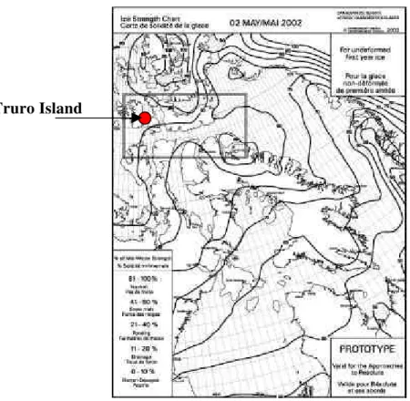
The preliminary ice strength algorithm was used by the CIS to generate prototype Ice Strength Charts (Gauthier et al., 2002). Figure 1 shows a representative Ice Strength Chart from May 2002. Since the prototype Charts were generated using a strength algorithm that was based upon measurements from one location (Truro Island, west of Cornwallis Island), the forecasted strengths were valid for ice in that area only. Although the ice strength algorithm was believed appropriate for regions of level first-year ice inside the box shown in Figure 1, there were no measurements to support using the ice strength algorithm for first year ice beyond Truro Island.

1

(13)

Because so little was known about ice decay in regions beyond Truro Island, one of the objectives of the third measurement season (2002) was to expand the scope of the decay work to include other areas of Parry Channel. It was envisioned that measurements made during the 2002 field season would establish the viability of using one strength algorithm for level, landfast first-year ice in Parry Channel.

Figure 1 Prototype Ice Strength Chart issued by Canadian Ice Service

3.0 Measured Ice Borehole Strength

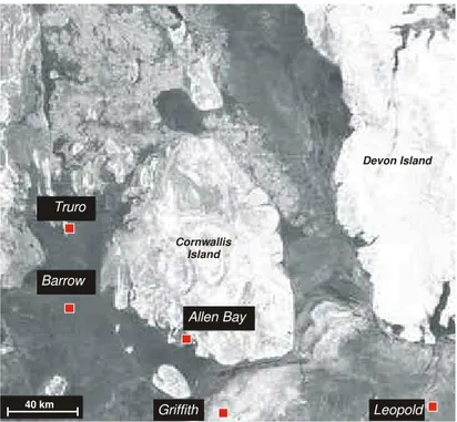
Figure 2 shows the areas of level, landfast first-year ice in Parry Channel that were sampled from 2000 to 2002. Ice decay measurements near Truro Island (75°13.9′N, 97°09.3′W) were made for three years. The four sites further east in Parry Channel, the so-called regional sampling sites, were sampled during the 2002 field season only. The regional sampling sites included Barrow (74°51.1′N, 97°07.4′W), Griffith (74°21.1′N, 94°51.3′W), Prince Leopold (74°19.5′N, 91°08.6′W) and Allen Bay (74°44′N, 95°15′W).

(14)

Allen Bay Truro Barrow Griffith Leopold Cornwallis Island Devon Island 40 km

Figure 2 Sampled first-year ice sites (January 2002 RADARSAT image courtesy of CIS)

3.1 Ice Borehole Strength: Past Measurement Seasons

Each season from May until July or August, the ice strength was measured using a borehole jack assembly. The borehole jack measured the confined, compressive strength of the ice, the so-called ice borehole strength. Details of the borehole jack system are provided in Johnston et al. (2003). Depth profiles of the ice strength in three different boreholes (separated by about 1.5 m) were obtained by testing at depth intervals of 0.30 m throughout the full-thickness of ice. The bulk strength of each hole was determined by averaging the strengths at each depth (depth-averaged). The site average strength (the three-hole mean) was obtained by averaging all measurements from all test holes at that site.

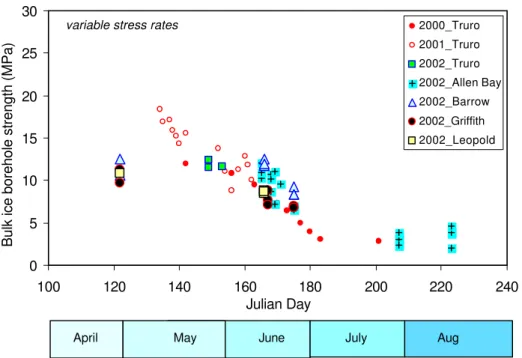
Figure 3 shows the depth-averaged, three-hole mean borehole strengths for the three measurement seasons. The figure shows good agreement between the borehole strengths of first-year ice at Truro and the regional sampling sites in Parry Channel. At all sites, the ice strength steadily decreased as the season advanced. The only exception to that trend was the 2 May (JD122) data from the Barrow, Griffith and Leopold sites. The early-May borehole jack tests at those sites produced strengths that were considerably lower than later in the season. The unusually low ice strengths resulted from malfunctioning equipment, which caused lower-than-normal loading rates.

The early May measurements showed the influence of loading rate on the measured ice strength. Making a rigorous comparison of ice strength for the different sites required accounting for that rate effect, which was done using the exponential relation between loading rate and ice strength described in Sinha (1986). Ice borehole strengths were standardized using a stress rate of 1.0 MPa/s, as discussed in Johnston et al. (2003).

(15)

0 5 10 15 20 25 30 100 120 140 160 180 200 220 240

Bulk ice borehole strength (MPa)

. 2000_Truro 2001_Truro 2002_Truro 2002_Allen Bay 2002_Barrow 2002_Griffith 2002_Leopold

June July Aug

April May

Julian Day

variable stress rates

Figure 3 Ice borehole strength in Central Arctic, varying stress rates

3.2 Temperature Dependence of Borehole Strength

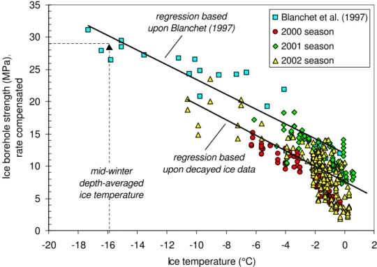
The rate-compensated borehole strength of decaying ice was most conveniently presented in terms of the maximum winter borehole strength of first-year ice. Blanchet et al. (1997) measured the borehole strength of cold, first-year ice at Tarsiut Island in the Beaufort Sea. Figure 4 shows the strengths2 of the Beaufort Sea ice as a function of ice temperature at the particular test depth, which ranged from –17.3°C to near 0°C. The corresponding rate-compensated borehole strengths ranged from 9.7 to 31.1 MPa. The figure shows the linear regression that was fit through the Blanchet et al. (1997) strength/temperature data.

Figure 4 also includes borehole strength and temperature measurements from the three decay seasons. The decayed ice measurements are shown for all depths in the three holes, based upon temperatures profiled from one of the extracted cores. The temperature of the decaying ice ranged from –10.5 to near 0°C and the corresponding borehole strength ranged from 1.9 to 23.5 MPa. A second, linear regression was fit through the strength/temperature measurements for decaying ice.

The figure shows that the ice borehole strength is inversely proportional to ice temperature. In winter, the surface layer of ice is colder and stronger than the warmer bottom ice. As a result, it is important to consider the full-thickness (bulk) strength of the ice, rather than the ice strength at one particular depth. Although the data in Figure 4 were obtained from individual test depths, they can be used to determine the depth-averaged borehole strength of winter ice, provided the average, full-thickness temperature of the ice sheet is known, as discussed subsequently.

2

Since the borehole jack tests in Blanchet et al. (1997) were conducted at stress rates from 0.2 to 0.5 MPa/s, those strengths were rate-compensated to 1.0 MPa/s before being compared to the CHC measurements on ice decay.

(16)

0 5 10 15 20 25 30 -20 -18 -16 -14 -12 -10 -8 -6 -4 -2 0 2 Ice temperature (°C)

Ice borehole strength (MPa),

rate compensated Blanchet et al. (1997) 2000 season 2001 season 2002 season mid-winter depth-averaged ice temperature regression based upon decayed ice data regression based upon Blanchet (1997)

Figure 4 Dependence of ice borehole strength upon ice temperature (all data rate compensated to 1.0 MPa/s)

3.3 Full-thickness Temperature of First-year Ice in Winter

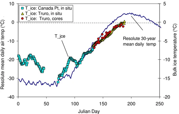
The full-thickness temperature of the ice sheet was determined using in situ temperature measurements made in level, first-year ice at Canada Point in Navy Board Inlet (73.7° N, 81.1°W). In the winter of 1984-85, a temperature chain was installed in the ice at Canada Point to measure hourly temperatures at depths 0.0, 0.25, 0.50, 1.0, 1.5 and 2.0 m (R. Frederking, personal communication). The Canada Point data provide a nearly continuous record of ice temperature from November to May. Measurements were not available from 16 February to 12 March (JD47 to JD71). Figure 5 shows full-thickness ice temperatures for first-year ice at Canada Point from November to May.

Ice temperature measurements from the three seasons of ice decay work were also included in the figure. The full-thickness temperature of the decaying ice was obtained from two sources: (1) temperatures measured from all cores extracted between 2000 and 2002 and (2) temperatures recorded in 2002 from the in situ temperature chain in the level ice near Truro Island (Johnston and Timco, 2002). There is excellent continuity between ice temperature measurements made at Canada Point (1984-85), the three years of processed cores (2000 to 2002) and in situ temperature measurements at Truro Island (2002).

(17)

-40 -30 -20 -10 0 10 0 50 100 150 200 250 Julian Day

Resolute mean daily air temp (°C) .

-20 -15 -10 -5 0 5

Bulk ice temperature (°C)

T_ice: Canada Pt, in situ T_ice: Truro, in situ T_ice: Truro, cores

Resolute 30-year mean daily temp T_jce

Figure 5 Influence of air temperature on the bulk (full-thickness) ice temperature

The 30-year average mean, daily air temperatures at Resolute are shown in Figure 5, relative to the full-thickness ice temperature. The mean daily air temperature at Resolute hovers around –30°C from January to early March, and then begins to increase steadily. Although Canada Point ice temperature data are missing from February until early March (JD47 to JD71), measurements show that the full-thickness temperature of the ice was beginning to increase by 12 March (JD71). Results showed that the minimum full-thickness ice temperature of –16.1°C occurred on 12 March (JD71), after two months of –30°C air temperatures. The minimum ice temperature was recorded immediately prior to the increase in the mean daily air temperature at Resolute.

3.4 Ice Borehole Strength: Winter Maximum

The Canada Point temperature data show that –16.1°C was the lowest full-thickness ice temperature measured from 1984-85. That temperature measurement was used in conjunction with Figure 4 to determine the maximum winter borehole strength of first-year ice. Figure 4 shows that, based upon the linear regression for winter ice and decayed ice, first-year ice with a full-thickness temperature of –16.1°C would have a borehole strength of about 29 MPa.

The Canada Point data were also used to determine the minimum full-thickness ice temperatures for winter and early spring. The monthly minimum temperature was used to determine the monthly maximum borehole strength from the data in Figure 4. Table 1 shows results from the correlation between the full-thickness ice temperature and borehole strength. Based upon the ice temperature data, the bulk borehole strength increases from 22 MPa in December to a maximum of 29 MPa in March. After March, the borehole strength begins to decrease. The maximum borehole strength in April is 24 MPa and 19 MPa in May.

(18)

Month Julian Day Full-thickness ice temperature, monthly minimum (°C) Ice borehole strength (MPa)† Normalized ice borehole strength December 357 -10.6 22 0.75 January 15 -11.5 23 0.79 February 43 -13.3 25 0.87 March 71 -16.1 29 1.00 April 104 -11.9 24 0.81 May 121 -8.4 19 0.65 †

strength corresponds to the monthly minimum temperature

4.0 Flexural Strength

The above discussion showed that the borehole strength, which is a measure of the confined compressive strength of the ice, is one way of quantifying the decay-related decrease in strength. The borehole strength provides a measure of the crushing strength of the ice. Ice crushing generates the highest loads during ice-structure interaction (Timco and Johnston, 2003).

The flexural strength of the ice is also an important component of ship-ice interactions. Depending upon a host of parameters, including bow form and ice thickness, the ice crushes until the flexural strength of the ice is exceeded and then fails in bending (or flexure). As a result, most ice-structure interactions are classified as mixed modal failures. Therefore, it is important to determine whether the flexural strength of the ice shows a decrease in strength similar to the trend observed in the borehole strength.

Changes in the flexural strength of the ice were investigated using the equation developed by Timco and O’Brien (1994). In their investigation, the authors used more than 2500 strength measurements from both polar and temperate regions to establish a relation between the flexural strength and brine volume. Their analysis resulted in the following equation;

) * 88 . 5 ( exp 76 . 1 _b f υ σ = − (1) where

σ ƒ = flexural strength (MPa) υb = fractional brine volume

The brine volume was calculated using the equation developed by Frankenstein and Garner (1967);         + = 49.185 0.532 i i b T S υ (2) where Si = ice salinity

(19)

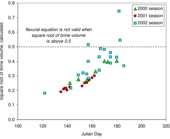
Using the model developed by Timco and O’Brien (1994), the flexural strength of the ice can be calculated from the full-thickness ice temperature and bulk ice salinity or, if those two ice properties are not known, from the air temperature and the ice thickness. Equation (1) has limitations, however. Since the equation is based upon the brine volume, it is only valid in the temperature range of –0.5 to –22.9°C. The flexural strength can only be used to calculate the ice strength up to a certain point because of the difficulty of accurately calculating the brine volume at near-melting ice temperatures.

The measurements included in Timco and O’Brien (1994) do not contain data to support using the relation between flexural strength and brine volume beyond a square root of brine volume of 0.5. Above a value of 0.5, the square root of brine volume becomes too large, causing inaccuracies in the calculated flexural strength and also the flexural strength measured in a test frame. Figure 6 uses ice property measurements from the three decay seasons to illustrate the point at which the square root of brine volume exceeds 0.5. When the full-thickness ice temperature and bulk salinity are used to calculate the brine volume, Equation (1) can be used until the end of June (JD180). However, if the bulk ice properties are not known, the flexural strength must be calculated using the air temperature and ice thickness. In that case, the flexural strength can only be calculated until air temperatures increase above freezing, which generally occurs in the high Arctic in early June (JD152), as shown by the mean daily air temperatures in Figure 5. 0.0 0.1 0.2 0.3 0.4 0.5 0.6 0.7 0.8 100 120 140 160 180 200 220 Julian Day

Square root of brine volume, calculated

2000 season 2001 season 2002 season

flexural equation is not valid when square root of brine volume

is above 0.5

(20)

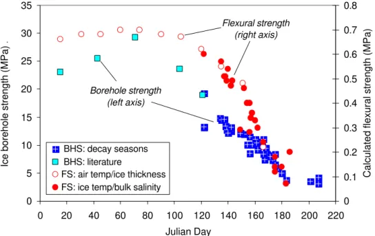
Since the borehole strength is a measure of the confined compressive strength of the ice, it is considerably larger than the unconfined flexural strength of the ice. For example, the maximum (winter) ice borehole strength is about 29 MPa (Figure 4), whereas maximum reported flexural strength for first-year ice is 0.71 MPa (Timco and O’Brien, 1994). The discussion below examines decay-related trends in the borehole and flexural strengths.

5.1 Measured Borehole Strength

The mid-winter borehole strengths shown in Figure 7 are the values reported in Table 1 (determined using Figure 4). Judging from borehole strengths in January (JD20) and March (JD71), the February borehole strength is lower than might be expected. This is because the ice temperature data from Canada Point were missing for two-weeks in February (from JD47 to JD60, see Figure 5). Had ice temperatures been recorded for the entire month of February, the ice would have been colder and its strength slightly higher.

Figure 7 includes borehole strength measurements from the three decayed ice programs. Those strengths represent the depth-averaged, three-hole mean borehole strength from each test site. Note the good agreement between the rate-compensated borehole strength of 19.2 MPa that was measured during the ice decay work on 2 May (JD122) and the borehole strength of 19 MPa that was determined using a minimum May full-thickness ice temperature of –8.4°C (from Table 1, in conjunction with Figure 4).

0 5 10 15 20 25 30 35 0 20 40 60 80 100 120 140 160 180 200 220 Julian Day

Ice borehole strength (MPa) .

0 0.1 0.2 0.3 0.4 0.5 0.6 0.7 0.8

Calculated flexural strength (MPa) .

BHS: decay seasons BHS: literature

FS: air temp/ice thickness FS: ice temp/bulk salinity

Borehole strength (left axis)

Flexural strength (right axis)

Figure 7 Seasonal decreases in measured borehole strength and calculated flexural strength

(21)

5.2 Calculated Flexural Strength

The flexural strength in Figure 7 was calculated first, from ice property measurements (full-thickness ice temperature and salinity) and second, from air temperature and ice (full-thickness measurements. The second technique was used in winter, when information about the bulk ice properties was not available. The winter air temperature and ice thickness data were obtained from 30-year mean daily air temperatures at Resolute and the measured ice thickness in Resolute (Bilello, 1960, 1980; Bilello and Bates, 1991; and Bilello and Lunardini, 1996).

Figure 7 illustrates what was stated earlier: the bulk ice properties can be used to calculate the flexural strength longer than air temperature and ice thickness measurements. The bulk ice properties provide information about the flexural strength until 2 July (JD183), whereas the air temperature and ice thickness can only be used when air temperatures are below freezing (prior to 8 June, JD159).

5.3 Comparison of Normalized Strengths

Figure 8-a shows the borehole and flexural strengths, normalized by their maximum winter values of 29 MPa and 0.71 MPa, respectively. Both the borehole and flexural strengths decrease from mid-March (JD74) to early July (JD183), however the calculated flexural strength decreases more slowly than the borehole strength until the first week of June (JD160). At present there is no explanation for the different trends, although it may relate to the value selected for the maximum winter borehole strength (full-thickness). Although measurements suggest a maximum winter borehole strength of 29 MPa (rate-compensated to 1.0 MPa/s), normalizing by a lower strength would have produced better agreement between the two strengths.

The inverse relation between the borehole strength and ice temperature supports the trend shown in Figure 8-a/b, namely that the bulk borehole strength decreases as the temperature of the ice warms throughout its full-thickness. The data suggest that the borehole strength first starts to decrease around 12 March (JD71), the point at which the ice begins to warm. By 2 May (JD122), the borehole strength was about 65% of its winter maximum. By the time above-freezing air temperatures were experienced in mid-June (JD165), the ice borehole strength had decreased to 30% of its maximum strength. Finally, by early July (JD183), the ice strength had decreased to 15% of its winter maximum. The ice strength remained at the 15% level until the last measurements were conducted in mid-August (JD223).

Comparison of the seasonal decrease in borehole strength and ice thickness measurements shows that whereas the borehole strength decreased from March to early June, the ice thickness continued to increase (Figure 8-a/b). Measurements showed that when the ice started to ablate in early June the ice had only 40% of its maximum winter strength. That is the point at which commercial shipping in the Arctic increases – when the level, landfast, first-year ice has only 40% of its winter strength and its thickness has started to ablate.

(22)

0.0 0.2 0.4 0.6 0.8 1.0 1.2 -100 -50 0 50 100 150 200 250 Julian Day

Normalized strength, ST_nor .

Calculated flexural strength Ice borehole strength

S O N D J F M A M J J A

(a) normalized strengths from September to August

-2.0 -1.8 -1.6 -1.4 -1.2 -1.0 -0.8 -0.6 -0.4 -0.2 0.0 -100 -50 0 50 100 150 200 250

Julian Day (January 1 = JD01)

Ice thickness, h_i (m) .

-20 -16 -12 -8 -4 0 4

Bulk ice temperature (°C)

bulk ice temp Canada Pt.

bulk ice temp decay work h_i at Resolute (from Bilello) h_i from decay work

(b) thickness and full-thickness temperature of the ice from September to August Figure 8 Normalized ice strength in relation to ice temperature and thickness

(23)

6.0 Relating Ice Strength to the Mean Daily Air Temperature

Having demonstrated that both the measured borehole strength and the calculated flexural strength show a seasonal decrease, the question of developing a methodology to predict the decrease in strength arises. The decay measurements showed that, despite the good agreement between three years of data, relating the decrease in ice strength to the time of year is not advised. That approach would not take into account inter-annual variability in climate, nor would it be feasible for incorporating other geographic regions into the analysis. A more effective technique would be to relate the decrease in ice strength to a well-known parameter, such as the mean daily air temperature.

6.1 Obtaining Mean Daily Temperatures from GEM Model

Considering that the number of weather stations in the Arctic is being reduced, it would not be wise to rely upon weather stations for air temperature data. Instead, quite a different approach was taken – air temperature data were output from the Global Environmental Multi-scale (GEM) forecast model used by the Canadian Ice Service. The model outputs air temperature data, twice per day (0000 and 1200 UTC), at an elevation of 10 m above sea level and at a resolution of 24 km.

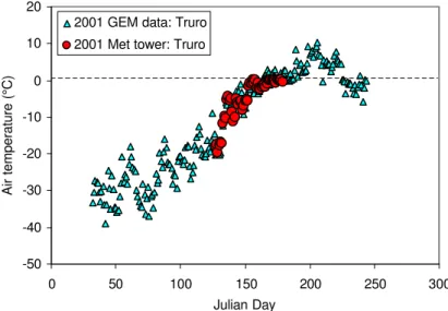
Figure 9 provides insight to the accuracy of mean daily air temperatures output from the GEM model (the two daily temperatures were averaged). The figure compares the 2001 average daily temperature from the GEM model (for Truro Island) to the mean daily air temperatures obtained from a temporary meteorological station, also located near Truro Island. Results show favorable agreement between air temperatures obtained from the two sources. A similar comparison was done for air temperature data from 2000. It also resulted in good agreement between the GEM temperatures and the meteorological station.

-50 -40 -30 -20 -10 0 10 20 0 50 100 150 200 250 300 Julian Day Air temperature (°C)

2001 GEM data: Truro 2001 Met tower: Truro

Figure 9 Mean daily air temperatures from GEM model (compared to meteorological data, 2001 season)

(24)

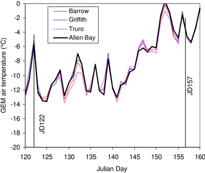
The high-resolution data output by the GEM model was used to compare air temperatures at each of the first-year ice sites sampled in Parry Channel during the 2002 decay season. Figure 10 shows the modeled air temperatures for each of sites for the arbitrary period 30 April to 9 June (JD120 to JD160). The GEM air temperatures at each of the sites were very close (at an elevation of 10 m). In comparison, the air temperatures measured at the different sites on the same sampling day in 2002 were quite different. When the ice at Barrow was sampled on 2 May (JD122, at 11:00) the air temperature was –11.4°C. In comparison, air temperatures were considerably warmer at the Griffith site, which was also sampled on 2 May (–4.1°C at 14:10). Similarly, on 6 June (JD157) the air temperature at Barrow was –1.0°C (at 18:00) whereas it was +1.7°C at Griffith (at 15:00). At present, there is no explanation for the different air temperatures obtained from spot field measurements and those temperatures output from the GEM model. -20 -18 -16 -14 -12 -10 -8 -6 -4 -2 0 120 125 130 135 140 145 150 155 160 Julian Day

GEM air temperature (°C)

Barrow Griffith Truro Allen Bay JD122 JD157

Figure 10 GEM mean daily air temperature data for sites in Parry Channel, 2002

7.0 2003 Strength Algorithm

The above discussion showed that since the high-resolution GEM model output temperatures that agreed favorably with those obtained from a meteorological station, the modeled temperatures could be used to establish a relation between the normalized ice strength and the mean daily air temperature. Two different approaches were used to explore that relation. First, the strength of first-year ice was directly related to the mean daily temperature – an approach that produced considerable scatter. Difficulties arose from the short-term increases in air temperature that may cause an under-predicted ice strength. Therefore, relating the ice strength directly to air temperature is not recommended.

(25)

7.1 Calculating the Accumulated Degree-Days (AWDD)

The preferred approach was to relate the strength of first-year ice to the accumulated degree-days (ADD). The ADD are determined by algebraically summing the mean daily air temperatures (Tmeandaily) using a specified start date (JD) and an appropriate baseline temperature

(Tbase). Once those two parameters have been selected, Equation (3) can be used to calculate the

ADD;

∑

− = JD base meandaily T T T ADD₍ _base₎ ( ) (3) where

ADD = accumulated degree-days Tmeandaily = mean daily air temperature

Tbase = baseline temperature from which ADD are calculated

JD = start date from which ADD are calculated

It should be noted that Equation (3) takes into account air temperatures that are both warmer and colder than the specified baseline temperature (Tbase). Following the procedure developed here,

the ADD will increase if air temperatures are warmer than the baseline temperature. In contrast, air temperatures that are colder than the baseline temperature, decrease the ADD.

7.2 Selecting a Baseline Temperature (Tbase)

In winter, the mean daily air temperatures at Truro hover around –30°C (Figure 9). Likewise, the mean daily air temperatures at Resolute are about –30°C in winter (Figure 5). Based upon that information, a baseline temperature (Tbase) of –30°C is appropriate for the high Arctic.

Should a different baseline temperature be used, it would change the magnitude of the ADD. For example, a baseline of –30°C results in a greater number of ADD than, say, a baseline of –10°C. That is because there would be a greater number of days on which the mean daily temperature exceeded –30°C than –10°C.

A baseline temperature (Tbase) of –30°C must be adhered to when using the relation

between the ice strength and ADD developed in this report.

7.3 Start Date used for Calculating Accumulated Degree Days (ADD)

Once the Tbase has been selected, the ADD must be algebraically summed from an appropriate

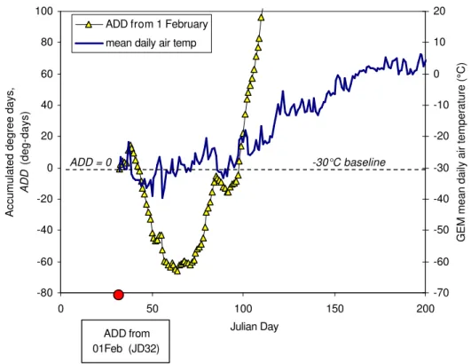
start date (Julian Day, JD). Initially, a start date of February 1 (JD32) was considered for the high Arctic. Using 1 February as a start date resulted in a bank of subtractive degree-days from 6 February to 1 March (JD37 to JD60), as shown by the values below the dotted line in Figure 11. Mean daily air temperatures colder than the baseline temperature of –30°C caused a

(26)

Tbase) was detrimental because it delayed the effect that ADD should have had on the decrease in

ice strength. Decreasing Tbase so that it was below the minimum mean daily air temperature did

not remedy the situation, because it caused the degree-days to begin accumulating about one month prior to the first decrease in ice strength (in early March, Figure 7).

-80 -60 -40 -20 0 20 40 60 80 100 0 50 100 150 200 Julian Day

Accumulated degree days,

ADD (deg-days) -70 -60 -50 -40 -30 -20 -10 0 10 20

GEM mean daily air temperature (°C) .

ADD from 1 February mean daily air temp

-30°C baseline

ADD from 01Feb (JD32)

ADD = 0

Figure 11 ADD calculated from 1 February (JD32), using a -30°C baseline

Figure 12 shows the ADD calculated from a start date of 1 March (JD60). The figure shows that a bank of subtractive degree-days did not develop for a start date of JD60. It was concluded that 1 March is a much better option for the high Arctic for the following reasons:

• the March 1 start date did not result in a bank of subtractive degree-days

• mean daily temperatures were consistently above a Tbase of –30°C after 1 March

• a start date of March 1 captured the decrease in ice strength, which was shown to occur around JD71 (Figure 8-a)

• the ADD were close to zero when the normalized ice strength began to decrease in early March

(27)

-80 -60 -40 -20 0 20 40 60 80 100 0 50 100 150 200 Julian Day

Accumulated degree days,

ADD (deg-days) -70 -60 -50 -40 -30 -20 -10 0 10 20

GEM mean daily air temperature (°C) .

ADD f om 01 March mean daily air temp

-30°C baseline

ADD from 01 Mar (JD60)

ADD = 0

Figure 12 ADD calculated from 1 March (JD60), using a -30°C baseline

The analysis outlined in this report was based on a start date of March 1 (JD60).

The same start date must be used when applying the strength-ADD relation

developed in this report.

7.4 Developing an Ice Strength Algorithm: Relating Ice Strength to ADD

The preceding discussion showed that the best option for determining the ADD from Equation (3) was to use a start date of 1 March (JD60) and a baseline temperature of –30°C. Since the ADD are used as the basis for relating the normalized ice strength (STnor) to the mean daily air

temperatures (Tmeandaily), a cross-plot of the two variables is shown in Figure 13. The data

included in that figure form the basis of the Ice Strength Algorithm for level, landfast ice in the high Arctic developed in this report.

Figure 13 shows that the maximum, normalized borehole strength of 1.0 corresponds to an ADD of zero. From that point forward, the normalized ice strength decreases with increasing ADD. The strength data in Figure 13 show the same sort of trend that was seen in earlier plots. That is, from March to June, the borehole strength decreases at a different rate than the flexural strength. Although the decrease in strength initially occurs at different rates, both data sets can be approximated by an exponential decay function.

(28)

0.0 0.1 0.2 0.3 0.4 0.5 0.6 0.7 0.8 0.9 0 500 1000 1500 2000 2500 3000 3500

ADD (deg-days), based upon threshold of -30°C

ST_nor, normalized ice strength

Borehole strength: winter Borehole strength: 2000 Borehole strength: 2001 Borehole strength: 2002 Flexural strength: 2000 Flexural strength: 2001 Flexural strength: 2002

Figure 13: Normalized strength versus the accumulated degree days, ADD

Three different exponential regression curves were used to relate the normalized ice strength to the ADD. The three curves are, in effect, three distinctly different algorithms, as shown in Table 2. Algorithm 1 was developed from both the borehole and flexural strength data (R² of 0.798). Algorithm 2 was developed using only the borehole strength data (R² of 0.897) and the third algorithm represented only the flexural strength data (R² of 0.879). Graphs of the three algorithms are included in Appendix B.

Table 2 Possible Strength Algorithms for First-year ice in the high Arctic

Algorithm No. Data sets used in developing algorithm

Algorithm

for normalized ice strength, STnor

Correlation coefficient

(R²)

1 Borehole and flexural

strengths (BHS & FS)

= 0.9114 exp (-0.0008 ADD) 0.798

2 Borehole strength only

(BHS only)

= 0.7390 exp (-0.0007 ADD) 0.897

3 Flexural strength only

(FS only)

(29)

8.0 Comparison of Predicted and Measured Strengths

Figure 14 compares the three algorithms to the normalized borehole strengths from three measurement seasons. The figure shows that Algorithm 1 (BHS and FS) and Algorithm 2 (BHS only) give a good approximation of the normalized borehole strength. Algorithm 1 better predicts the decrease in strength from ADD 0 to 500, however Algorithm 2 is more representative of the decrease in strength from ADD 500 to 1000. Since Algorithm 1 and Algorithm 2 are virtually identical beyond an ADD of about 1000, either could be used to predict the decrease in strength after an ADD of 1000. Algorithm 2, which is based upon solely the calculated flexural strength data, is a poor measure of the decease in borehole strength. Results show that Algorithm 3 would overestimate the ice strength early in the season and under-predict it later in the season.

0.0 0.2 0.4 0.6 0.8 1.0 1.2 0 500 1000 1500 2000 2500 3000 3500 ADD (deg-days)

ST_nor, normalized strength, predicted

BHS measured Algorithm 1: BHS & FS Algorithm 2: BHS only Algorithm 3: FS only flexural strength only borehole strength only

borehole and flexural strengths

Figure 14 Predicted and measured strength relative to ADD

Having determined that Algorithm 3 was not appropriate for predicting the decrease in ice strength, it was necessary to decide which of the remaining algorithms (Algorithm 1 or 2) offers a better approach for relating the ADD to ice strength. Figure 15 presents a comparison of the measured borehole strength and the strength forecasted using Algorithm 1 and Algorithm 2 (both strengths are normalized). The literature-derived winter borehole strengths were not included in the plot, so as not to bias strengths measured during the three decay seasons, which is the area of most interest. A dotted line is used to show a 1:1 correspondence between the measured and forecasted strengths. Algorithm 2 has a slightly better correlation (R² of 0.865) between the measured and forecasted strengths than Algorithm 1 (R² of 0.856). However, the figure shows that by overestimating the ice strength, Algorithm 1 provides a margin of safety – something that Algorithm 2 does not have.

(30)

0.0 0.2 0.4 0.6 0.0 0.2 0.4 0.6 0.8 ST_nor , measured ST_nor , predicted _{Algorithm 2} (R² = 0.865) Algorithm 1 (R² = 0.856)

Figure 15 Cross plot of predicted and measured, normalized ice strength

Due to its margin of safety, Algorithm 1

(31)

9.0 Summary and Conclusions

Analysis showed that the normalized strength (STnor) of level, landfast first-year ice in the high

Arctic can be forecasted using the following algorithm:

) 0008 . 0 ( exp 9114 . 0 ₍ ₎ base T nor ADD ST = − (4)

where ADD, the accumulated degree-days, is calculated using a Tbase of –30°C, as show below;

∑

− − = ° − 60 ) 30 ( ( ( 30)) JD meandaily C T ADD (5)

In generating Ice Strength Charts, the analysis should:

• calculate the ADD starting from March 1 (JD60)

• use a threshold temperature, Tbase, of -30°C and

• include both positive and negative contributions to the ADD

Three seasons of measurements on decayed first-year ice were used to develop an Ice Strength Algorithm for relating the normalized ice strength to the ADD. An Ice Strength Algorithm was suggested for forecasting the strength of level, landfast first-year ice in the high Arctic during the decay season. Results showed favorable agreement between the measured and forecasted ice strengths, particularly from mid-May to August. Good correlation between the measured and forecasted ice strength from early to late summer is important from a shipping perspective, since most commercial shipping in the Arctic occurs from June to August. Analysis showed that the forecasted ice strengths will be most accurate when information about the ice strength is needed most, in mid- to late summer.

The start date and baseline temperature are fundamental to calculating ADD. Since those two parameters were deemed appropriate for the high Arctic, the suggested Ice Strength Algorithm is only appropriate for first-year ice in that region. The Canadian Ice Service has the objective of developing a strength algorithm for forecasting the seasonal decrease in strength of first-year ice at more southerly latitudes (R. DeAbreu, personal communication). Preliminary investigation showed that a single Strength Algorithm is not likely to be appropriate for all geographic regions, nor is much known about the effect that snow cover has on temperature changes in the ice. Further work will need to be conducted in these areas before an Ice Strength Algorithm can be developed for sub-Arctic ice.

(32)

10.0 Acknowledgements

This work was funded by the Canadian Ice Service. Their financial support and assistance in conducting field measurements at the distributed sampling sites in Parry Channel are most appreciated.

11.0 References

Bilello, M.A. (1960) Formation, Growth and Decay of Sea Ice in the Canadian Arctic Archipelago. U.S. Army Snow Ice and Permafrost Research Establishment Special Report. No. 65. July, 1960. 19 pp.

Bilello, M.A. (1980) Maximum Thickness and Subsequent Decay of Lake, River and Fast Sea Ice in Canada and Alaska. CRREL Report No. 80-6. February, 1980. 160 pp.

Bilello, M.A. and Bates, R.E. (1991) Ice Thickness Observations, North American Arctic and Subarctic, 1972 – 73 and 1973 – 74. CRREL Special Report. No. 43, VIII. December, 1991. 127 pp.

Bilello, M.A. and Lunardini, V.J. (1996) Ice Thickness Observations, North American Arctic and Subarctic, 1974 – 75, 1975 – 76 and 1976 – 77. CRREL Special Report. No. 43, IX. May, 1996. 221 pp.

Blanchet, D., Abdelnour, R. and Comfort, G. (1997) Mechanical Properties of First-year Sea Ice at Tarsiut Island. Jour. of Cold Regions Engineering, Vol. 1, pp. 59-83.

Frankenstein, G.E. and Garner, R.. (1967) Equations for Determining the Brine Volume of Sea Ice from –0.5 to –22.9 C. Jour. of Glac. Vol. 6, No. 48, pp. 943 – 944.

Gauthier, M-F., DeAbreu, R., Timco, G.W. and Johnston. M. (2002) Ice Strength Information in the Canadian Arctic: From Science to Operations. Proceedings IAHR Ice Symposium, Dunedin, New Zealand, pp. 203 - 210.

Johnston, M., Frederking, R. and Timco, G. (2002) Properties of Decaying First-year Sea Ice: Two Seasons of Field of Field Measurements. Proceedings 17th International on Okhotsk Sea and Sea Ice, Mombetsu, Hokkaido, Japan, pp 303 - 311.

Johnston, M. and Timco, G. (2002) Temperature Changes in First-year Arctic Sea Ice during the Decay Process. Proc. Int. Sym. on Ice (IAHR), Dunedin, New Zealand, Vol. 2, pp. 194 – 202.

Johnston, M, Timco, G. and Frederking, R (2003) Decay Processes in Arctic First-year, Second-year and Multi-Second-year Sea Ice. in preparation.

Sinha, N.K. (1986) The Borehole Jack: Is it a Useful Tool? Proc. of 5th Int. Offshore Mechanics and Arctic Engineering Symp. (OMAE). Tokyo, Japan. 13 – 17 April 1986. Vol. IV. pp. 328 – 335.

Timco, G.W. and Johnston, M. (2003) Ice Loads on the Molikpaq in the Beaufort Sea. Jour. of Cold Regions Engineering, in print.

Timco, G.W. and O'Brien, S. (1994) Flexural Strength Equation for Sea Ice. Jour. Cold Regions Science and Technology, Vol. 22, pp. 285 – 298.

(33)

(34)

(35)

(36)

2003 Ice Strength Algorithm:

Changes made to Previously Developed Algorithm, March 2002

• Analysis included the 2002 borehole measurements and flexural strength calculations

• Flexural strength data used in the normalized strength–ADD relation were calculated using full-thickness ice temperatures and salinity measurements, rather than from air temperatures and ice thicknesses

• ADD were calculated using average daily air temperatures from 0000 and 1200 UTC output from the high-resolution GEM model, rather than the global model (1 degree resolution)

• 2000 season: Truro GEM temperatures

• 2001 season: Truro GEM temperatures

• 2002 season: average of Truro, Barrow, Allen Bay and Griffith GEM temperatures

• ADD were calculated using a –30°C baseline, as with last year

• ADD were algebraically summed starting from March 1, rather than April 1

• included the winter borehole strength measurements in determining an exponential decay function for the normalized borehole strength data

(37)

(38)

Appendix B Comparison of Measured Ice Borehole Strength and Predicted

Strengths

(39)

(40)

ST_nor = 0.9114e-0.0008ADD R² = 0.7975 0.0 0.2 0.4 0.6 0.8 1.0 0 1000 2000 3000 4000

ADD (deg-days), using threshold of -30°C

STnor, normalized strength

BHS & FS: normalized

(a) Algorithm 1: borehole strength and flexural strength

St_nor = 0.739e-0.0007ADD R² = 0.8969 0.0 0.2 0.4 0.6 0.8 1.0 0 1000 2000 3000 4000

BHS: normalized

(b) Algorithm 2: borehole strength only

ST_nor = 1.7412e-0.0012ADD R² = 0.8794 0.0 0.2 0.4 0.6 0.8 1.0 0 1000 2000 3000 4000

FS: normalized

(41)

(42)

Comparison of Measured and Predicted Ice Strengths for Three Algorithms, 2002 data only ST_nor AWDD JD 2002 Measured BHS Algorithm 1 (BHS & FS) Algorithm 2 (BHS only) Algorithm 3 (FS only) 321.65 122 0.66 0.70 0.59 1.18 321.65 122 0.38 0.70 0.59 1.18 321.65 122 0.29 0.70 0.59 1.18 854.06 149 0.45 0.46 0.41 0.62 1298.80 165 0.25 0.32 0.30 0.37 1330.06 166 0.22 0.31 0.29 0.35 1330.06 166 0.46 0.31 0.29 0.35 1360.73 167 0.29 0.31 0.29 0.34 1392.92 168 0.41 0.30 0.28 0.33 1392.92 168 0.36 0.30 0.28 0.33 1425.21 169 0.33 0.29 0.27 0.31 1488.76 171 0.32 0.28 0.26 0.29 1614.58 175 0.29 0.25 0.24 0.25 1614.28 175 0.27 0.25 0.24 0.25 1614.58 175 0.22 0.25 0.24 0.25 2659.51 207 0.14 0.11 0.11 0.07 2659.51 207 0.11 0.11 0.11 0.07 3165.37 223 0.13 0.07 0.08 0.04

(43)