The Economics of Software Development by Pair Programmers

Publisher’s version / Version de l'éditeur:

Engineering Economist, 48, 4, 2003

READ THESE TERMS AND CONDITIONS CAREFULLY BEFORE USING THIS WEBSITE.

https://nrc-publications.canada.ca/eng/copyright

Vous avez des questions? Nous pouvons vous aider. Pour communiquer directement avec un auteur, consultez la première page de la revue dans laquelle son article a été publié afin de trouver ses coordonnées. Si vous n’arrivez pas à les repérer, communiquez avec nous à PublicationsArchive-ArchivesPublications@nrc-cnrc.gc.ca.

Questions? Contact the NRC Publications Archive team at

PublicationsArchive-ArchivesPublications@nrc-cnrc.gc.ca. If you wish to email the authors directly, please see the first page of the publication for their contact information.

Archives des publications du CNRC

This publication could be one of several versions: author’s original, accepted manuscript or the publisher’s version. / La version de cette publication peut être l’une des suivantes : la version prépublication de l’auteur, la version acceptée du manuscrit ou la version de l’éditeur.

Access and use of this website and the material on it are subject to the Terms and Conditions set forth at

The Economics of Software Development by Pair Programmers

Erdogmus, Hakan; Williams, L.

https://publications-cnrc.canada.ca/fra/droits

L’accès à ce site Web et l’utilisation de son contenu sont assujettis aux conditions présentées dans le site LISEZ CES CONDITIONS ATTENTIVEMENT AVANT D’UTILISER CE SITE WEB.

NRC Publications Record / Notice d'Archives des publications de CNRC:

Institute for

Information Technology

Institut de technologie de l'information

The Economics of Software Development by

Pair Programmers *

Erdogmus, H., and Williams, L.

2003

* published in The Engineering Economist, 48(4): 33. 2003. NRC 47101.

Copyright 2003 by

National Research Council of Canada

Permission is granted to quote short excerpts and to reproduce figures and tables from this report, provided that the source of such material is fully acknowledged.

T

HE

E

CONOMICS OF

S

OFTWARE

D

EVELOPMENT BY

P

AIR

P

ROGRAMMERS

H

E

National Research Council, CANADA

L

W

North Carolina State University, USA

ABSTRACT

Evidence suggests that pair programmers—two programmers working collaboratively on the same design, algorithm, code, or test—perform substantially better than the two would working alone. Improved quality, teamwork, communication, knowledge management, and morale have been among the reported benefits of pair programming. This paper presents a comparative economic evaluation that strengthens the case for pair programming. The evaluation builds on the quantitative results of an empirical study conducted at the University of Utah. The evaluation is performed by interpreting these findings in the context of two different, idealized models of value realization. In the first model, consistent with the traditional waterfall process of software development, code produced by a development team is deployed in a single increment; its value is not realized until the full project completion. In the second model, consistent with agile software development processes such as Extreme Programming, code is produced and delivered in small increments; thus its value is realized in an equally incremental fashion. Under both models, our analysis demonstrates a distinct economic advantage of pair programmers over solo programmers. Based on these preliminary results, we recommend that organizations engaged in software development consider adopting pair programming as a practice that could improve their bottom line. To be able to perform quantitative analyses, several simplifying assumptions had to be made regarding alternative models of software development, the costs and benefits associated with these models, and how these costs and benefits are recognized. The implications of these assumptions are addressed in the paper.

INTRODUCTION

Both anecdotal and statistical evidence [1-4] indicate that pair programming, the practice whereby two programmers work side-by-side at one computer collaborating on the same design, algorithm, code or test, is highly productive. One of the programmers, the driver, has control of the keyboard/mouse and actively implements the design, program, or test. The other programmer, the navigator, continuously observes the work of the driver to identify tactical (syntactic, spelling, etc.) defects and also thinks strategically about the direction of the work. On demand, the two programmers brainstorm any challenging problem. Because the two programmers periodically switch roles, they work together as equals to develop software. Many have used the pair programming technique for decades, and several publications in the mid-late 1990s extolled its benefits [1, 5, 6]. More recently, many impressive anecdotes among those practicing the Extreme Programming (XP) software development methodology [7-11] greatly aroused awareness of pair programming as a technique to improve quality, productivity, knowledge management, and employee satisfaction [3, 4, 12].

In 1999, a formal experiment was run to investigate the effectiveness of the pair programming practice. The experiment was run with advanced undergraduates at the University of Utah. Sometimes issues of external validity are raised when empirical software engineering studies are conducted with students. These issues arise because projects undertaken within a semester in artificial settings need not deal with matters of scope and scale that often complicate real, industrial projects. However, academic settings are still valuable as test-beds. They have the potential to provide sufficient realism at low cost while allowing for controlled observation of important project parameters [13].The University of Utah empirical study focused on the interactions between and the overall effectiveness of two programmers working collaboratively relative to programmers working alone. Issues of complexity and scale are not significant inhibitors in such a study.

Software development methodologies, or processes, are prescribed, documented collections of software practices (specific methods for software design, test, requirements documentation, maintenance, and other activities) required to develop or maintain software. Williams developed the Collaborative Software ProcessSM (CSPSM) methodology as her dissertation research [14]. CSP is based on Watts Humphrey’s well known Personal Software ProcessSM (PSPSM) [15], but is specifically designed to leverage the power of two

programmers working together. The University of Utah experiment assessed the effectiveness of solo programming using the PSP vs. the effectiveness of pair programmers using the CSP. These two processes were specifically chosen to best isolate the effects of pair programming; essentially all the other practices followed by the programmers were identical. The experiment yielded statistically significant differences between the performance of pair programmers and of individual programmers [3, 4, 14, 16]. In this paper, these experimental results are used to perform a quantitative analysis of the economic feasibility of pair programming. The findings complement and strengthen the benefits of pair programming that have been reported previously.

The economic feasibility of pair programming is a key issue. Many instinctively reject pair programming because they believe code development costs will double: why should two programmers work on each task while a single programmer can do the job? If the practice is not economically feasible, managers simply will not permit its use. Organizations decide whether to adopt process improvements based on the bottom-line implications of the outcomes. Naturally, the goal of software firms is to be as profitable as possible while providing their customers with the highest-quality products as quickly and cheaply as possibly.

The economic feasibility analysis of the pair programming practice centers on how it fares relative to solo programming under a given value realization model. We assume a product realizes value when clients or end users are delivered a working product. Even a partial, but working, product can provide benefits. We will compare pair programming with solo programming first based on simple performance metrics, and then considering these metrics under two different value realization models. In the latter case, the analysis utilizes Net Present Value (NPV) [17] as the basis for comparison. This approach per se is not novel. Economic models based on NPV have previously been suggested to evaluate the return on software quality and infrastructure initiatives; for examples, see [18-22]. Our analysis stands out in that it relies on a breakeven analysis instead of a traditional NPV analysis.

ASSUMPTIONS

The economic feasibility of pair programming is assessed by focusing on the performance of a single pair of programmers with respect to the performance of a solo programmer. The comparison is made under the assumption that both the paired programmers and the solo programmer are undertaking the same

programming task. Whether the solo or pair programmers work in isolation or are part of a larger team is thus immaterial at this level of comparison.

Our economic assessment makes a number of other simplifying assumptions. Some of these assumptions abstract away from extraneous factors over which the programmers normally have no control, while others reduce the number or limit the behavior of the underlying variables in order to make a quantitative comparison possible:

• Cost accumulation. Labor cost is the only kind of cost considered. All costs are recognized instantly as they are accrued. One-time overhead costs, such as the pair jelling time [4], are disregarded. (Pair jelling is the time period in which programmers learn to work effectively in a pair, to give and to accept objective suggestions, and to communicate during development.) Since we compare a single programming pair to a single programmer working alone, the pattern of expenditures for labor costs is linear in each case: costs are accrued continuously and at a constant rate.

• Work schedule. Programmers work a fixed number of work hours per year. Work hours are evenly distributed within a calendar year. During work hours, programmers never remain idle and exclusively engage in development activities, either writing new code or fixing defects in previously deployed code.

• Defect recovery process. The post-deployment defect discovery process is assumed to be perfectly efficient. This implies that after a piece of code has been deployed, all defects are found instantly. We assume that post-deployment defects are found by the clients or users of the deployed code, and not by the programmers. Since programmers are never idle during work hours, the defect discovery time irrelevant from the programmers’ perspective. All discovered defects are repaired at a fixed rate by the original programmers, but the average speed with which they are repaired depends upon the development process used.

• Value realization. A linear relationship is assumed between the amount of code deployed by the programmers and the value generated through the development activity. Deployed code

instantly realizes value when it is defect-free. Code may be deployed in arbitrarily small increments.

• Ranges and baseline values of model parameters. Whenever necessary and reasonable, statistics previously reported in the literature are used to determine the ranges and baseline values of model parameters.

ABSTRACTION OF THE DEVELOPMENT PROCESS

The two development processes that underlie the comparison are the Personal Software Process (PSP), which is designed for individual programmers, and the Collaborative Software Process (CSP), which is designed for pair programmers. The CSP practices are intentionally based on PSP practices, with the exception of pair programming. As a result, we consider that our comparison of PSP and CSP is essentially a comparison between solo and pair programming. The shared practices of the two processes, therefore, are not discussed here.

In what follows, we refer to a single programmer or a team of programmers simultaneously working on a piece of code as a work unit. We represent the development process in terms of two descriptive and three empirical parameters. The size of the work unit uniquely differentiates the CSP from the PSP.

MEASURES OF TIME AND EFFORT:

Elapsed time refers to the delta between the times of occurrence of two events.

Compressed time refers to elapsed time minus overhead and resting time. Effort refers to equivalent compressed time for a single programmer. Thus if a work unit is composed of a single programmer, effort equals compressed time. If it is composed of a pair of programmers, effort equals twice the compressed time.

We measure elapsed time in years, compressed time in hours, and effort in

person-hours. From now on, hours always refer to productive hours, that is, time spent exclusively on development activities excluding overhead and resting time. Labor costs are calculated based on effort, or productive person-hours.

If a programmer works on average 7.5 productive hours per day, 5 days a week, and 49 weeks a year, he or she works a total of 1,837.5 person-hours in a calendar year. In this case, 1,837.5 person-hours of effort are equivalent to 1,837.5 hours of compressed time, which in turn are equivalent to one year of elapsed time. However, for a pair of programmers, 3,675 person-hours of effort are equivalent to 1,837.5 hours of compressed time, or a year of elapsed time.

DESCRIPTIVE PARAMETERS:

The two descriptive parameters of the development process are:

• Size of the work unit (N, persons). The number of programmers in a work unit. N equals 1 for a solo programmer (hereby, a soloist), and 2 for a pair of programmers (hereby, a pair). Thus N = 1 if the work unit consists of a soloist following the PSP. N = 2 if the work unit consists of a pair of programmers working in tandem on the same task following the CSP.

• Value realization model. The pattern in which a work unit delivers a finished or partial product, and accordingly generates value. This parameter will be discussed later in the paper.

The work unit (N) and the value realization model are the only independent parameters in the process model. The values of the empirical parameters all depend on N.

EMPIRICAL PARAMETERS:

Before we introduce the empirical parameters, we need to define how we measure the output (denoted by ω) of a work unit. A work unit, depending on how efficient it is, is able to produce only a certain amount of output within a given time. Conversely, a work unit, again depending on its efficiency, requires a certain amount of time to produce a given amount of output. In the latter case, the output targeted by the work unit can be thought of as the size of the of the development task undertaken. In other words, it may be thought of as an external requirement on the work unit.

In software development, output is an elusive concept to represent and measure. Output is, by and large, a subjective notion whose interpretation is the cause of much controversy. To be meaningful, the measure of output should correlate with how much technical functionality is provided by the software artifact produced. Yet there is no universally accepted way of counting technical functionality. We use the most widely adopted and easy to compute measure,

lines of code (LOC). However, LOC is just a proxy. Some argue that LOC is not an appropriate measure of output in that LOC may not always correlate well with the amount of functionality delivered. More abstract measures, such as function points, have been suggested as alternatives, but these are not suitable in our analysis because of their coarse and non-uniform granularity.

The unit of two empirical parameters, productivity and defect rate, depend on the adopted unit of output. If LOC is substituted by another output measure, the units of productivity and defect rate will change accordingly.

Having defined output, the three empirical parameters of the development process are:

• π: productivity (LOC/hour). The average hourly output of the work unit, measured in compressed time.

• β: defect rate (defects/LOC). The average number of defects per unit of output (per LOC) produced by the work unit.

• ρ: rework speed (defects/hour). The speed at which the work unit repairs defects in a piece of previously deployed code, after the defects have been discovered. Also measured in compressed time.

The values of these three parameters are determined empirically based on past research studies and statistics reported in the literature. The chosen values are primarily for illustration purposes, and represent information available at the time of writing. The actual values could be different, and they would most likely be both project- and skill-dependent. The specific results reported here are sensitive to the empirical parameters to varying extents, however we believe that the general conclusions are much less so under the assumptions of the analysis. A sensitivity analysis is performed at the end of the paper.

PRODUCTIVITY :

According to a study by Hayes and Over [23], the average productivity rate of 196 developers who took PSP training was 25 LOC/hour. This figure will be the chosen value of π for N = 1 (soloist). Note that the developers in the PSP training course were essentially free from normal business interruptions. As a result, this figure may seem high when compared with other productivity figures based on monthly rates in which programmers’ total output is compared with their total time (including meetings, absences, vacation, etc.). However, the Hayes and Over productivity figure is appropriate for our analysis as we use compressed time to measure productivity.

The University of Utah study [4, 14] reported that a pair spends on average only 15% more effort (in total person-hours) than a soloist to complete the same programming task. This result however was not statistically significant, with approximately a 40% probability of the observed difference in the mean being due to chance. Although further analysis was not performed on the data set to verify whether the two-tailed t-test employed was powerful enough to detect the

difference at the specified alpha level in the first place, anecdotal evidence [2, 7, 10]is supportive of no significant total effort penalty for pair programmers after pair jelling has occurred [4, 24, 25]. In our firsthand observations, there is a one-time jelling cost of between one to 40 hours the first time a programmer pairs. Subsequently, there is another short 30-60 minute jelling period when a programmer pairs with a different programmer for the first time; during this time the programmers learn each other’s strengths and weaknesses relative to their own.

We err on the conservative side by assuming that the observed 15% difference is real. With this assumption, in a single person-hour, each programmer of a pair produces an average of 25/(1.15) = 21.74 LOC, and together they produce twice this volume, or 43.48 LOC. Thus, benchmarked relative to the baseline PSP productivity level of 25 LOC/hour, the value of π for N =2 (pair) is taken to be a conservative 43.48 LOC/hour.

These pair productivity rates are within 20-30% of those recently reported by a technology company in India that used both pair and solo programming in a Voice-over-IP project. This project reported a pair-to-soloist productivity ratio of 2.8 (3300 LOC/month for solo programmers versus 9600 LOC/month for pair programmers based on a 60-hour work week) [26]. Note that this ratio is much higher compared to the more conservative ratio of 1.73 adopted here.

DEFECT RATE :

According to Jones [27], code produced in the US has an average of 39 raw defects per thousand LOC (KLOC). This statistic is based on data collected from such companies as AT&T, Hewlett Packard, IBM, Microsoft, Motorola, and Raytheon,with formal defect tracking and measurement capabilities. According to the same reference, on average, 85% of all raw defects are removed via the development process, and 15% escape to the client.

Together the two pieces of statistics suggest an average post-deployment defect rate of (0.039)(0.85) = 0.00585 defects/LOC (or 5.85 defects/KLOC). The number is consistent, though on the low side, with data from the Pentagon and the Software Engineering Institute, which indicate that typical software applications contain 5-15 defects per KLOC [28]. We adopt the average 0.00585 defects/LOC as the baseline soloist value of β, for N = 1.

During the empirical study of pair programming vs. solo programming, Williams [3, 4, 14, 16]observed that at the end of the project, code written by pairs on average passed 90% of the specified acceptance tests compared to code written by soloists, which passed on average only 75% of the same test suite. The results were statistically significant at an alpha level of less than .01.

Assuming that the test suite provided full coverage, this result suggests a pair-to-soloist post-deployment defect rate ratio of .6 (corresponding to an improvement of 1 − .6 = 40%). Thus benchmarked relative to the soloist (N = 1) baseline value of 0.00585 defects/LOC, the adopted value of β for a pair (N = 2) is (0.00585)(0.6) = 0.00351 defects/LOC.

The adopted soloist value of β is close to the average defect rate of 0.00534 defects/LOC reported by the Indian company mentioned previously [26]. However, for pairs, the company reported defect rates that are an order of magnitude lower than the adopted β value of 0.00351 defects/LOC, both during unit testing (at 0.0002 defects/LOC) and during acceptance testing (at 0.0004 defects/LOC), corresponding to an improvement of over 90% over soloists. In the initial analysis, we will err on the conservative side again by adopting the figures yielded by the University of Utah study. Later in the paper, sensitivity analysis will show how an improvement as dramatic as the one reported by the Indian company affects the results.

REWORK SPEED :

A study of a set of industrial software projects from a large telecommunications company [29] reported that each discovered (post-deployment) defect required an average of 4.5 person-days, or 33 person-hours of subsequent maintenance effort or rework (based on a 7.5-hour workday). This statistic is consistent with data reported by Humphrey [15]. Based on this observation, the value of rework speed ρ for a soloist (N =1) is taken to be 1/33 = 0.0303 defects/hour. Again this figure serves as our baseline value for computing the pair rework speed.

No data is available regarding the effect of pair development on rework activities. We will assume pairs can achieve rework productivity gains comparable to those reported for the initial development activities. Under this assumption, the estimated rework speed ρ for a pair (N = 2) will be (2)(0.0303)/1.15 = 0.0527 defects/hour. This assumption would especially be valid for agile development processes [30, 31] such as Extreme Programming [8], where no clear separation exists between rework and development activities. INITIAL ABSTRACT MODELS:

For now we leave the value realization model unspecified since it will not be needed for the initial comparison. Thus the initial abstract models that represent the two development processes are:

Pair = {N = 2, π = 43.478, β = 0.00351, ρ = 0.0527}.

Note that pair jelling costs [4, 24, 25] have been excluded in this model. At this point, we have no viable empirical data beyond the anecdotes discussed above regarding jelling costs. Exclusion of jelling costs injects a bias into the analysis in favor of pair programming. If jelling cost is a one-time cost, this bias should not be significant. However if it is recurring due to pair rotation or turnover, it should be factored into the productivity parameter to eliminate the bias. Fortunately, productivity is the least sensitive of the three empirical parameters. This helps reduce the bias in the analysis.

THE BASIC COMPARISON MODEL

The basic comparison model consists of three metrics: efficiency, unit effort, and unit time.

EFFICIENCY:

Efficiency, ε, is defined as the percentage effort spent on developing new code,

exclusive of the effort expended on rework. Given a productivity rate of π, the effort required to produce ω lines of code of output is given by:

:= E_pre ω N

π

This quantity specifies the initial development (or pre-deployment) effort. Initial development is followed by rework (or post-deployment) effort once the code has been deployed (fielded, or delivered to the client). Rework effort, Epost,

refers to the maintenance effort expended to repair runaway defects after a piece of new code has been deployed and all such defects have been found.

:= E_post ω β N_ρ

Here ωβ is the total number of defects and ρ is the speed of rework. Effort is always adjusted to the work unit by multiplying it by the work unit’s size N.

Total effort, Etot, is the sum of the initial development and rework efforts:

:=

E_tot ω N (ρ β π + ) π ρ

Efficiency, ε, is then the ratio of the initial development effort Epre to the

total effort Etot. It is thus given by:

=

ε ρ

+ ρ β π

The percentage effort spent on rework then equals 1 − ε, or:

β π + ρ β π

It may seem counterintuitive at first that efficiency and productivity are inversely related. Why should increasing productivity reduce efficiency? It is because under a constant defect rate, the number of post-deployment defects increases with output. Therefore, all other parameters remaining same, an increase in productivity results in a higher number of total post-deployment defects, increasing the rework effort, and ultimately decreasing the percentage effort spent on initial development.

Some development techniques allegedly increase productivity while reducing the defect rate at the same time. For example, agile development processes claim to achieve this [8]. If such is the case, simultaneously, a reduction in βπ and an increase in ρ will result, and consequently efficiency will increase.

UNIT EFFORT :

Unit effort, UE, is the total effort, in person-hours, required by a work unit to produce one unit (LOC) of defect-free output. UE is calculated by dividing total effort Etot by the total output ω corresponding to that effort. Expressed in terms

of productivity and efficiency, unit effort is given by:

:=

UE N

π ε

UNIT TIME:

Unit time, UT, is the compressed time, in hours, required by a work unit to produce one unit (LOC) of defect-free output.

Unit time is calculated by dividing unit effort UE by the size of the work unit N. Expressed in terms of productivity and efficiency, unit time equals:

:= UT 1

π ε

RESULTS OF BASIC COMPARISON MODEL:

Table 1 compares the two abstract models Solo and Pair with respect to the metrics efficiency, unit effort, and unit time. In each row, the cell in bold typeface indicates the more favorable alternative with respect to the corresponding metric. The model Pair fairs considerably better in all of the three metrics, yielding nearly 100% improvement in efficiency, over 40% reduction in unit effort, and over 70% reduction in unit time.

Table 1. Comparison of the models Solo and Pair based on performance metrics.

Model

Metric

Solo Pair

Efficiency (ε) (decimal %) .172 .340

Unit Effort (UE) (person-hours/LOC) .233 .135

Unit Time (UT) (hours/LOC) .233 (= UE) .068

THE ECONOMIC COMPARISON MODEL

A software development activity incurs costs as it accumulates labor hours and realizes value as it delivers new functionality to the clients or the users of the end product. The activity is economically feasible when the total value it creates exceeds the total cost it incurs. We assume that the net value generated depends on four factors: (1) the activity’s labor cost; (2) the value that the activity earns commensurate with the output it produces; (3) the way in which this earned value is recognized, or realized, through a specific pattern of deploying the output produced; and (4) the discount rate r used to bring the underlying cash flows to the present time. The economic comparison model takes into account the effect of each of these factors.

LABOR COST:

Programmer labor is often the most important cost driver in software development. Let Cpre and Cpost denote the average labor cost of initial

benefits. We will assume that initial development and rework are performed by the same work unit, resulting in the same constant value for both variables. Thus:

Cpre= Cpost= C

In the economic comparison model, we account for labor costs as such costs are incurred, in a similar fashion a business using accrual-based accounting would recognize expenses when they are transacted. However, to avoid choosing an arbitrary period for transacting labor costs, we assume instead that these costs are accrued in a continuous manner as a series of infinitesimally small transactions.

DISCOUNT RATE:

When the costs and benefits of an activity are spread over a long period of time, the economic analysis must take into account, in addition to their magnitude, the specific times at which these costs and benefits are recognized as concrete cash flows. To maximize net economic value, the activity should realize benefits as early as possible and incur costs as late as possible.

We assume that the resulting cash flows are discounted at a fixed continuously-compounded annual rate r from the time of their occurrence relative to the start time of the activity. The various interpretations of the discount rate—for example, in terms of opportunity cost, time value of money, project risk, minimum required rate of return, or any combinations thereof—are beyond the scope of this paper. We refer the unfamiliar reader to the standard capital budgeting literature; for example, see the relevant chapter in Ross [17]. EARNED VALUE:

Earned value (EV) is a well known quantitative project tracking method [15, 20, 32, 33]. With EV tracking, a project’s expected outputs or resources are estimated and scheduled for delivery or consumption, respectively. As the project progresses, it earns value relative to this delivery/consumption schedule, so that at completion, the project’s earned value equals the total estimated output or the total estimated consumption. For example, a project with a target to produce 100 units of a product would have a current EV of 20 after producing 20 units. With a target of 200 units, after producing the same amount of units, it would have an EV of 10. In both cases, every unit produced increases the accumulated EV by a fixed amount: by one unit in the former case, and by half a unit in the latter. Let this constant incremental value be denoted by V. We refer

to V, the value earned by one unit of output, as the unit value. In our case, V corresponds to the average currency value of a single line of code, expressed in $/LOC. Then earned value corresponding to a total output of ω LOC is given by:

EV = V ω

According to our economic model, not every labor hour expended earns value. Effort, such as rework, that does not increase output or result in new functionality does not earn any value. Therefore our interpretation of earned value considers rework effort as wasted effort. Consequently, only projects that are 100% efficient earn extra value for each labor hour expended.

VALUE REALIZATION:

In software development, earned value is not necessarily the same as

realized value. The distinction between the two is important. Earned value can be seen more as an expression of potential value commensurate with effort spent given the productivity level of the development team. That value however may never be realized, for example if the project fails to deliver a useable artifact. Potential value is realized when an artifact leaves production and is delivered to its client. This can be accomplished in small increments or in large chunks over the course of a software development project. The rate at which realized value accumulates depends on the frequency with which working code fragments are deployed to the client. Hence although value can be earned on a continuous basis, possibly it is not realized until much later.

The concept of realized value may also be explained in reference to the two alternative methods of income recognition seen in the Generally Accepted Accounting Principles [34]. In cash-based accounting, income from services rendered is recognized when services are paid for; while in accrual-based accounting, income from services are recognized when services are delivered. Thus the concept of realized value admits an accrual-based view of value recognition rather than a cash-based view: new code is developed, deployed, and reworked in increments of different size, and as such, realized value is accumulated at the same pace as obligations regarding these increments are fulfilled.

In the economic analysis, we consider two alternative value realization models: single-point delivery (value realized at the end) and continuous

These two models are located at the opposite extremes of the value realization spectrum. The contrast helps demonstrate the impact of the pattern of value realization on the economic feasibility of a process. Most real projects fall somewhere in between these two theoretical extremes. In contract-based development, the terms of the contract dictate the actual value realization pattern. New contracting models with novel compensation structures are being put forward for software projects; for example, see Beck and Cleal [35]. The model we use in our analysis can easily be adapted to a particular compensation model.

The Single-Point Delivery Model

With traditional, waterfall-like [36] models of software development, code delivery to the client often occurs in one large chunk. The scope of the development activity is fixed and finite. Hence, value is realized in a single step at the very end. We will refer to this value realization model as single-point

delivery, or deferred realization.

The single-point delivery model is illustrated in Figure 1. The horizontal dimension denotes elapsed time with respect to a single project. Here, we ignore the time it takes for the client or users to discover and report the defects in the deployed code. Therefore in this simple model, the rework phase immediately follows the development phase, and once all post-deployment defects are repaired, the project is deemed complete. In Figure 1, time τ marks project completion. It also marks the time of the realization of value accumulated over the course of the project. During rework, from τpre to τ, the

project does not earn any extra value.

Development

τpre τ

Start Deploy Complete

Rework

Figure 1: Single-point delivery model of value realization.

Incremental Delivery Model

At the opposite end of the spectrum is the incremental delivery model. In this model, the scope of the development activity need not be predetermined, and the

responsibility of the work unit may extend to perpetuity. New code is continuously developed, deployed, and reworked in small increments. Development of new code and rework of deployed code are intertwined in a never-ending cycle. Consequently, value is realized in small increments as micro-obligations involving small chunks of new code are gradually fulfilled.

The generic incremental delivery model is illustrated in Figure 2. Again, the horizontal dimension represents elapsed time. The ticks correspond to deployment points at which the work unit delivers new working code. In the idealized version of the incremental delivery model, the distance between two subsequent deployment points approaches to zero, giving rise to a truly continuous process. We will consider this idealized version only, which we refer to as the continuous delivery model. The idealized model avoids the selection of an arbitrary increment size.

Start

Rework

…

Deploy Deploy Deploy Deploy Deploy Rework Rework ReworkRework

Figure 2: Incremental delivery model of value realization.

DEFECT DISCOVERY:

We define a (post-deployment) defect as a runaway fault that the work unit was

unable to discover and remove prior to the deployment of a piece of code. These defects are rather discovered by the client of the code, be that the end user or a separate quality assurance team. The efficiency of the defect discovery process depends on two components: latency and coverage.

Latency refers to the elapsed time between the deployment of a software artifact and the discovery of a defect by the client of the artifact. Coverage refers to the number of defects reported by the client or users in relation to the total number of defects remaining in the code base.

In practice, the discovery of defects by the client is neither instantaneous nor complete. For example, Jones [27] states that in large industrial projects, more than half of the runaway defects have a latency of one year, while total coverage four years after deployment hovers around 97%. In contrast, agile software development processes, such as Extreme Programming and SCRUM [37], that rely on short cycles, continuous testing, and frequent client feedback, would tend to have low latency and high coverage.

The economic analysis performed here assumes a perfectly efficient defect discovery process: one with zero latency and full coverage. This allows us to abstract away from factors outside the control of the work unit.

Zero-latency is of little concern. First, latency does not affect the work unit’s obligation. Second, we assume that the work unit always has work to do. Thus if at a specific time, the programmers are not able to work on a specific piece of code, they won’t remain idle, but rather will undertake another development task, whether from the same or from another project. Therefore, the results of an analysis performed with zero-latency assumption should remain valid when averaged across several staggered development activities with non-zero latency.

Low coverage reduces the obligation of the work unit: fewer reported defects amount to less rework effort for the work unit. However, coverage is also a common environmental factor: it should affect pairs and soloists in the same manner. The effect of less-than-perfect coverage may be accounted for by converting actual defect rates into coverage-adjusted, effective defect rates. If coverage is constant, its impact, if any, can therefore be analyzed through a sensitivity analysis of the actual defect rates.

DEVELOPMENT OF THE ECONOMIC COMPARISON MODEL

NET PRESENT VALUE:

The Net Present Value of an investment activity is the difference between the present value (PV) of the activity’s benefits and the present value of its costs. This definition is adapted to the current context by representing the benefits in terms of realized value, accrued in a specific pattern, and the costs in terms of labor expenses, accrued continuously. With this adaptation, NPV becomes sensitive to changes in the unit value V.

Figure 3 shows how NPV varies as V varies in the neighborhood of 5% to 30% of the unit labor cost C for a pair under the single-point delivery model. NPV is represented by the vertical axis. Output is plotted in KLOCs. The labor cost C is set to 50 and a work schedule with hy = 1837.5 hours/year is assumed.

Figure 3: NPV as a function of unit value V and output ω for a fixed annual discount rate r = 10%.

In the figure, the NPV = 0 plane splits the V-Output space into feasible (NPV > 0) and infeasible (NPV < 0) regions. The range of V is chosen to emphasize the behavior of NPV in the neighborhood of this feasibility plane. Note that the slope of the NPV curve changes drastically along the output axis as

V varies. Because of this sensitivity, our interest is not in NPV per se. We need a derived metric whose value can be used to rank two alternatives independent of a particular choice of unit value. Breakeven Unit Value meets this need.

BREAKEVEN UNIT VALUE—ARELATIVE RETURN-ON-INVESTMENT METRIC:

Breakeven Unit Value is the threshold value of V above which the NPV is positive:

BUV = min{ V | NPV ≥ 0 }

BUV is determined by solving the equation NPV = 0 for V. Recall that V is measured in $/LOC, and represents the fixed increase in earned value per each additional unit of output produced.

A small BUV is better than a large BUV. As its BUV increases, the development activity becomes less and less worthwhile because higher and higher margins are required to move the NPV into the feasible region. Think of BUV as a relative measure of return on investment.

BREAKEVEN UNIT VALUE RATIO (BUVR):

Using BUV ratios, it is possible to make a one-step comparison between two development processes and gauge their relative feasibility. Define BUV Ratio (BUVR) as the ratio of the BUV of the model Solo to the BUV of the model Pair under a common value realization model.

= BUVR

BUV_solo BUV_pair

Values of BUVR greater than unity indicate an advantage for pairs; values smaller than unity indicate an advantage for soloists. As this ratio increases, the advantage of pairs over soloists also increases.

The metric BUVR makes the comparison not only independent of V, but also of the hourly labor cost C. BUVR depends on:

• the empirical parameters of the models Solo and Pair, • the value realization model, and

• in the case of the single-point delivery model, the discount rate and the total output (or the size of the development task undertaken).

SUMMARY OF THE ECONOMIC COMPARISON:

Table 2 summarizes the results of the economic comparison. The process models Solo and Pair are compared under two opposite value realization models with respect to the BUVR metric. The two value realization models considered are:

1. the single-point delivery model and

2. the idealized version of the incremental delivery model, or the

continuous delivery model.

In Table 2, r denotes the annual discount rate. Projects of higher risk usually require the use of a proportionately higher discount rate. Note that we apply the same discount rate for both negative cash flows (costs) and positive cash flows (benefits). In practice, costs and benefits may be subject to different levels and types of risk, possibly warranting the use of different discount rates. A detailed discussion of the relationship between risk, return, and discount rate is beyond the scope of this paper, but can be found in an introductory corporate finance text; for example, see [17].

In the single-point delivery model, BUVR depends both on the discount rate and the total output produced by the development unit. In general, as the

discount rate and output increase, BUVR, hence the advantage of the pair over the soloist, increases (with a slightly positive second partial derivative). In the continuous delivery model, the BUVR is constant and greater than unity, representing a steady advantage for pairs.

The limit behaviors are described by the rows “ω → ∞” (development continues to perpetuity) and “r → 0” (discount rate is zero). The final row of the table specifies whether the pair or the soloist fares better under each of the two value realization models.

Overall, a pair operating under the continuous delivery model yields the lowest (thus best) BUV since this model combines the improved efficiency and productivity of the pair with the advantage of incremental value realization. This observation highlights the impact of the value realization model on the economic analysis.

The findings are however sensitive to the three empirical parameters π (productivity), β (defect rate), and ρ (rework speed) to varying degrees. The most sensitive empirical parameter is the defect rate, followed by the rework speed, and finally the productivity. Sensitivity is discussed in more detail later in the paper.

Table 2. Economic comparison of models Solo and Pair based on BUVR.

BUVR Behavior Value Realization Condition Model Single-Point Delivery Continuous Delivery Discount rate (r) increases BUVR increases

r → 0 BUVR → 2.24

Output (ω) increases BUVR increases

ω → ∞ BUVR → ∞

BUVR = 1.73

Overall better model Pair Pair

BENEFITS AND COSTS IN SINGLE-POINT DELIVERY:

We now explain the elements of the economic analysis for the single-point delivery model in more detail. When value is realized only at the end of a development activity, NPV can be written as:

:=

Here DRV denotes Deferred Realized Value and TDC Total Discounted

Cost. Each of these quantities is discussed in detail below.

Deferred Realized Value

Deferred Realized Value (DRV) is the accumulated earned value at the end of the development activity expressed in present value terms. DRV is given by:

:=

DRV V ω e(−r τ)

where Vω = EV is the total deferred earned value; τ is elapsed time to completion; and r is the fixed, continuously compounded annual discount rate. The factor e(-rτ) brings the deferred EV to the present time.

Expressing τ in terms of output ω and the empirical parameters, DRV becomes: := DRV Vω e ⎛ ⎝ ⎜⎜ ⎜ ⎞ ⎠ ⎟⎟ ⎟ −_{π ε h}rω y

where π is the process (work unit) productivity (LOC/hour), ε is the process (work unit) efficiency (unitless), and hy describes the work schedule in terms of the total number of productive labor hours in a calendar year. The factor hy converts compressed time in hours to elapsed time in years based on a fixed work schedule. When needed, we assume a work schedule with hy = 1,837.5 hours per year, based on a 5-day workweek, 7.5-labor-hour workday, and 49-workweek year.

An optimal value of output exists that maximizes the deferred realized value. This value of output is defined by the root of the partial derivative of DRV with respect to ω:

= ∂

∂

ωDRV 0

Maximum DRV is given by:

= DRV_max Vπ ε h ye (-1) r

Note that maximum DRV increases with efficiency, but decreases with discount rate. Since V, hy, and, r are constant, the maximum DRV ratio of a soloist to a

pair is simply given by (πsolo εsolo)/(πpair εpair) = UTpair/UTsolo, yielding a constant value of 0.29. Therefore, the maximum value realizable under the single-point delivery model by a soloist is less than one third of the maximum value realizable by a pair. The maximum DRV ratio is thus independent of unit value and discount rate.

Marginal Cost

Marginal cost is the cost accumulated by a work unit per unit of elapsed time. For the single-point delivery model, marginal cost before and after deployment will be different if hourly labor cost for initial development and rework are different. We will first calculate a total discounted cost based on this general case, and then use the assumption Cpre = Cpost to simplify the result.

Considering a period of τ years in elapsed time and a process (work unit) efficiency of ε, the Marginal Initial Development Cost in dollars per year is given by:

:= mC_pre

Eε C_pre

τ =hyNε Cpre

Similarly, the Marginal Rework Costin dollars per year is:

:= mC_post

E (1 − ε C) _post

τ = −hyN(− + 1 ε C) post

The total discounted cost can now be calculated from these two components.

Total Discounted Cost

We assume that labor costs are accrued on an ongoing basis. This is a reasonable assumption since corporations incur payroll cash flows in regular discrete installments, for example, on a weekly, bi-weekly, or monthly basis. We discount labor costs as soon as they are incurred. In reality, these costs are recognized in a discrete manner, but when the time horizon is sufficiently long, a continuous model provides a frequency-independent approximation.

With these considerations in mind, the Total Discounted Cost for the model Solounder single-point delivery is obtained by summing the marginal costs accumulated over infinitesimally small intervals, both before and after deployment:

:= TDC₁ ⌠ d + ⌡ ⎮ ⎮ ⎮ 0 τ pre mC_pree(−r t) t ⌠ d ⌡ ⎮ ⎮ ⎮ τ pre τ mC_post e(−r t) t

Here mCpre dt and mCpost dt represent initial development and rework costs, respectively, accumulated over a small interval dt in the neighborhood of t. The factor e(−rt)brings the small cash flow that occurs over dt to the present time by discounting it over the period t. The variable of integration, t, represents elapsed time.

When Cpre = Cpost = C, the sum of the two integrals reduces to:

h_yN C(−2ε e + − + + ) (−r τ ) pre ε e(−r τ) e (−r τ ) pre ε e(−r τ) r By substituting = τ _{π ε h}ω y = τ_pre ω π h_y

in the previous equation, it is possible to express TDC in terms of total output ω, efficiency ε, and productivity π.

BUV in Single-Point Delivery

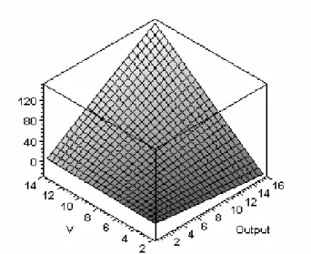
Under the single-point delivery model, BUV depends on both output (ω) and discount rate (r). It increases as either of these variables increases. Figure 4 shows the BUV for the model Pair under single-point delivery, for a fixed labor cost of C = $50/hour and a work schedule with hy = 1837.5 hours/year. BUV increases with output as well as with discount rate as a result of deferred value realization under the single-point delivery model, where higher and higher profit margins are required as total time to completion increases.

Figure 4: Breakeven Unit Value for the model Pairunder single-point delivery for a fixed hourly labor cost and work schedule. Output is in KLOCS.

When the discount rate is zero, BUV in the single-point delivery model is given by: = lim → r 0 BUV₁ (1 − 2ε 2 ε + ) 2 N C π ε

The limit yields a constant minimum BUV both for a pair and for a soloist. BUVR in Single-Point Delivery

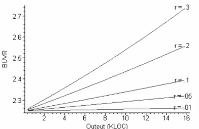
The economic advantage of pairs over soloists is evident in the single-point delivery model. BUVR is at least 2.24 when the discount rate is zero; the BUV for a soloist is at least 124% higher than the BUV for a pair. The pair’s advantage increases as output or discount rate increases. The effect is illustrated in Figure 5, which plots Solo to Pair BUVR as a function of total output for different discount rates under single-point delivery. Pairs accumulate costs faster, but more than compensate for this by realizing the deferred total value earlier. The bigger the development task or the higher the discount rate, the more pronounced is the advantage of pairs over soloists.

As Figure 5 demonstrates, BUVR is not very sensitive to changes in the discount rate although BUV itself is (Figure 4). Taking the ratio smoothes the impact of discount rate out to a certain degree. For example, even at high values of output (for large projects), a six-fold increase in the discount rate increases

the BUVR by less than 19%. Below an output of 5 KLOC (for small projects), BUVR increases by less than 6%.

Figure 5: BUVR of the model Solo to the model Pairunder single-point delivery as a function of output for different discount rates.

BENEFITS AND COSTS IN CONTINUOUS DELIVERY:

We now explain the elements of the economic analysis for the continuous delivery model in more detail. For the continuous delivery model, NPV is expressed as:

:=

NPV_∞ IRV − TDC_∞

Here IRV denotes Incremental Realized Value, and TDC again denotes

Total Discounted Cost.

Marginal Value Earned

Marginal Value Earned (MVE) is the average value earned by the work unit per additional unit of elapsed time (measured in $/year). Given a cutoff time of τ, again measured in elapsed time, MVE equals:

:=

Representing output ω in terms of elapsed time eliminates the variable τ, allowing MVE to be expressed as a function of unit value V, productivity π and efficiency ε:

:=

MVE Vπ ε h

y

Incrementally Realized Value

Incrementally Realized Value (IRV) is the total value earned over a given time period. Since value is realized, or recognized, as it is earned in the continuous delivery model, it is discounted continuously as earned. If τ is a time period measured in elapsed time, then IRV accumulated over τ is given by:

:= IRV ⌠ d ⌡ ⎮ ⎮ 0 τ MVE e(−r t) t

As usual, the variable of integration, t, is measured in elapsed time. Expressed in terms of efficiency ε and productivity π, IRV equals:

:= IRV −

Vπ ε h_y(e(−r τ) − 1) r

As the cutoff time τ approaches infinity, IRV asymptotically approaches its maximum value. This limit represents the value of operating a single work unit to perpetuity under a constant discount rate. Maximum IRV is given by:

=

IRV_max Vπ ε hy r

As with maximum Deferred Realized Value, maximum IRV increases with efficiency and decreases with discount rate.

With the current values of empirical parameters, pairs achieve 53% higher maximum IRV than soloists. Since the discount rate (r), the unit value (V), and the number of labor hours in a calendar year (hy) are the same for both soloists and pairs, the to-soloist ratio of maximum IRV is given directly by the pair-to-soloist ratio of efficiency.

Marginal Cost

Marginal cost was defined as the incremental cost of development and rework per additional unit of elapsed time. This definition is the same as it was in the single-point delivery model, but its computation is slightly different here. Since under continuous delivery, initial development and rework activities are intertwined, marginal cost, mC∞, can be written in terms of total effort E as:

:= mC_∞

+

Eε C_pre E(1 − ε C) _post τ

When Cpost = Cpre = C, marginal cost simply reduces to:

=

mC_∞ h

yN C

Total Discounted Cost

As is the case in the single-point delivery model, under the continuous delivery model, labor costs are accrued and discounted continuously to calculate the TDC. If the variable t represents elapsed time, TDC can be written as the following integral: := TDC_∞ ⌠ d ⌡ ⎮ ⎮ ⎮ 0 τ mC_∞e(−r t) t

After substituting the marginal cost with the corresponding term, the above definite integral reduces to:

:= TDC_∞ −

h_yN C(e(−r τ) − 1) r

Maximum Discounted Cost

The Maximum Discounted Cost of a work unit under the continuous delivery model at a constant discount rate is the asymptotic value of TCD incurred by the work unit to perpetuity. This limit is given by:

= TDC_{∞ max,}

h_yN C r

A pair consistently incurs twice the maximum discounted cost incurred by a soloist. This is because the ratio of maximum TDC is determined solely by N, as the labor cost (C) and the discount rate (r) are assumed to be the same for both practices.

BUV in Continuous Delivery

When both value realization and cost accumulation are continuous and incremental, BUV’s dependence on output and discount rate is broken in the continuous delivery model. Generically, BUV under the continuous delivery model is given by:

:= BUV_∞ N C

π ε

This equation yields, for a fixed labor cost of C = $50/hour, a Breakeven Unit Value of 11.65 for the model Solo and 8.96 for the model Pair.

BUVR in Continuous Delivery

The BUVR in continuous delivery is given by:

= BUVR_∞

N_solo π_pairε_pair N_pair π_soloε_solo

The value of BUVR is thus constant at 1.73 under this model of value realization, representing a steady 42% (1 − 1/1.73) advantage for pairs over soloists. Note that this advantage is independent of the discount rate and total output.

SENSITIVITY ANALYSIS OF THE ECONOMIC COMPARISON MODEL

Figure 5 illustrated the sensitivity of the BUVR to the two exogenous parameters—namely the discount rate (r) and output (ω). In the single-point delivery model, BUVR was found to be mildly sensitive to both discount rate and output. In the continuous delivery model, BUVR is constant.

How sensitive are the findings to the three endogenous, empirical parameters, productivity (π), rework speed (ρ), and defect rate (β)? Since these parameters are descriptive of the development process and the work unit, they

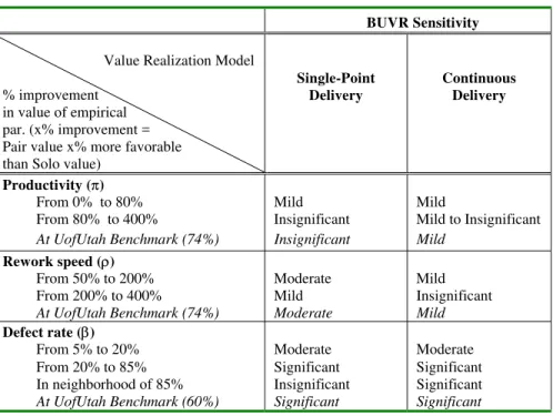
warrant further investigation. BUVR turns out to be most sensitive to changes in defect rate, but less so to changes in rework speed. It is least sensitive to changes in productivity. Table 3 provides further details on the sensitivity analysis.

Table 3. Sensitivity of BUVR to changes in empirical parameters. BUVR Sensitivity

Value Realization Model % improvement

in value of empirical par. (x% improvement = Pair value x% more favorable than Solo value)

Single-Point Delivery

Continuous Delivery

Productivity (π)

From 0% to 80% Mild Mild

From 80% to 400% Insignificant Mild to Insignificant At UofUtah Benchmark (74%) Insignificant Mild

Rework speed (ρ)

From 50% to 200% Moderate Mild From 200% to 400% Mild Insignificant At UofUtah Benchmark (74%) Moderate Mild Defect rate (β)

From 5% to 20% Moderate Moderate From 20% to 85% Significant Significant In neighborhood of 85% Insignificant Significant At UofUtah Benchmark (60%) Significant Significant

In Table 3, we characterize the sensitivity of BUVR to an empirical parameter over a given range as insignificant if the partial derivative of BUVR with respect to the percentage increase in that variable over the range in question is hovering around zero; mild if the absolute value of the partial derivative is consistently less than unity, but above zero; moderate if the absolute value is hovering around unity; and significant if it is consistently greater than unity. The columns in italics typeface indicate the sensitivity of the empirical parameters at the improvement levels achieved by pairs relative to soloists according to the data from the University of Utah study. These values serve as benchmark improvement levels for the purposes of the sensitivity analysis.

In Figures 6 through 8, for the production of the plots, we maintained the discount rate and the output at the arbitrary values of 0.1 (10%) and 7.5 KLOC, respectively. Staying within reasonable ranges, varying these exogenous parameters only marginally displaces the curves and does not affect the sensitivity results with respect to the three empirical parameters.

SENSITIVITY OF BUVR TO IMPROVEMENT IN PRODUCTIVITY:

Figure 6 illustrates the sensitivity of the findings to the level of improvement in productivity (π) achieved by pairs over soloists. The percentage improvement is expressed relative to the previously-adopted benchmark productivity value of 25 KLOC/hour, the productivity value used in the model Solo.

Both comparisons are initially mildly sensitive to improvement in productivity. The sensitivity decreases as the productivity improvement increases. Around the benchmark improvement level of 74% (dotted line), the effect is insignificant for single-point delivery and mildly significant for continuous delivery.

SENSITIVITY OF BUVR TO IMPROVEMENT IN REWORK SPEED:

Figure 7 illustrates the sensitivity of the results to the level of improvement in rework speed (ρ) achieved by pairs over soloists. The percentage improvement is expressed relative to the adopted benchmark rework speed value of 0.0303 defects/hour, again the value used in the model Solo in the main part of the analysis.

Overall, BUVR is mild to moderately sensitive to rework speed. Both comparisons exhibit a diminishing sensitivity to improvement in rework speed. In single-point delivery, a marginal increase in the rework speed of pairs relative to that of soloists provide a matching benefit up to an improvement level of around 200%, which we characterize as moderate sensitivity. At the benchmark level of 74% (dotted line), the effect is moderately sensitive for single-point delivery and mildly sensitive for continuous delivery.

1 ∞

1 – Single-point delivery ∞ – Continuous delivery

Figure 6: Sensitivity of BUVR to improvement in productivity.

1

∞

1 – Single-point delivery ∞ – Continuous delivery

Figure 7: Sensitivity of BUVR to improvement in rework speed.

SENSITIVITY OF BUVR TO IMPROVEMENT IN DEFECT RATE:

Figure 8 illustrates the sensitivity of the results to the level of improvement in defect rate (β) achieved by pairs over soloists. The percentage improvement is

expressed relative to the adopted benchmark defect rate of 0.00585 defects/LOC, the value used in the model Solo in the main part of the analysis. Unlike in rework speed and productivity, an improvement in defect rate corresponds to smaller, not larger, values of β. A maximum improvement of 100% corresponds to a defect rate of zero.

Overall, BUVR is initially moderately sensitive to changes in defect rate, and then becomes increasingly sensitive to it. Around the benchmark improvement level of 60%, the effect is significant. A deviation from this behavior occurs around the 85% neighborhood for single-point delivery. In this neighborhood, the BUVR peaks and then starts to decline. The peaking effect is attributed to the increasing double labor cost of pairs finally overtaking the diminishing savings from reduced rework effort. The peaking effect is absent in continuous delivery, because the advantage of incremental value realization is persistent.

1 ∞ 1 – Single-point delivery

∞ – Continuous delivery

Figure 8: Sensitivity of BUVR to improvements in defect rate.

We conclude the sensitivity analysis with a note on the impact of less-than-perfect defect coverage. When defect coverage is less than 100%, but constant, the effective defect rate will be lower than the actual defect rate, but by the same

factor for both pairs and soloists. This leaves unaffected the ratio of the pair defect rate to that of the soloist. Consequently, the percentage improvement in β, hence the value of BUVR, remains the same.

CONCLUSIONS,LIMITATIONS, AND FUTURE WORK

Quantitative analyses demonstrate the potential of pair programming as an economically viable alternative to individual programming. We compared the two practices under two different value realization models. In each case, we found that pair programming creates superior economic value based on data from a previous empirical study and other statistics reported in the general software engineering literature. Although the techniques and concepts employed in the analysis are standard, their use in this particular type of assessment, especially the incorporation of value realization considerations into a breakeven analysis, is novel.

In both practices, net value is maximized when the development activity realizes value incrementally, for example, through frequent releases. This observation is consistent with the general engineering economics intuition [20]. The more interesting question that was addressed by the analysis is how fast a development activity can afford to spend before the rate of spending overtakes the benefits of early value realization.

The results have low sensitivity to the two exogenous parameters: output and discount rate. Neither parameter was found to be a significant determining factor. Among the endogenous parameters, productivity and rework speed exhibit mild to moderate sensitivity, but neither of these parameters alone appears to be powerful enough to affect the comparison.

The findings were particularly sensitive to defect rate, the third endogenous parameter. However, everything else being the same, the advantage of pair programming persists until the defect rate ratio falls significantly, from the benchmark level of 60% down to 20%. The sensitivity to defect rate is not particularly surprising, since the case for pair programming largely hinges on a significant improvement in code quality.

Our observation confirms that further studies of pair programming should focus on measuring and comparing defect rates.

The analyses performed relied on several assumptions. The main ones were: 1. exclusion of overhead costs;

3. quality bias, due to rework effort being regarded as wasted effort; 4. ability to deliver a product in arbitrarily small increments; 5. a perfectly efficient defect discovery process.

Assumptions 2 and 5 abstract away from context-specific and environmental factors common to both practices of which the work unit has no or little control. Assumption 3 is important to retain because removing it would create a disincentive for poor quality. These three assumptions apply to both pair programming and solo programming equally, and were necessary for a context-independent comparison of the two practices. Assumptions 1 and 4 may however be relaxed at the expense of additional model complexity.

Other considerations include following:

• The disconnect between realized value and business value. We used earned value rather than business value as a proxy for benefits. The inclusion of business value would be meaningful only in concrete contexts because business value depends on project- and market-related factors. Business value can be tackled by redefining realized value independently of earned value, in terms of a separate exogenous parameter. An earlier version of the economic model adopted this view, however, we did not find it suitable for a generic analysis. • Treatment of more realistic value realization models that fall between

the two extremes addressed. Intermediary models can be tackled by breaking up development along an orthogonal dimension with two components: initial release and subsequent releases. The frequency of subsequent releases can be used as a sensitivity parameter to determine an optimal release cycle. Again, this kind of treatment is most useful if different alternatives are evaluated in a concrete context, rather than for a general comparison.

• More sophisticated characterizations of the empirical models.

Sensitivity analyses provide much insight when the empirical models are sufficiently well described by the mean values of the parameters involved. When these parameters are subject to high-levels of variability from one organization or project to another or within a single project, and the parameters exhibit mutual dependencies, their joint distributional properties become important. If empirical data can be used to infer these properties, probabilistic analyses can be performed at the lowest level. Sensitivity analyses can then be

performed at the next level to gauge the impact of errors in the descriptive parameters of the hypothesized distributions.

• Second-order interactions among individual practices. It is possible for the substitution of one practice for another (in this case, pair programming for solo programming) to have unintended, but systematic effects in the rest of the practices shared by two development processes (in this case, CSP and PSP). Such second-order interactions could amplify or dampen the observations. Although the University of Utah study did not report effects of this kind, it is still possible that they existed, but were not detected by the study. Second-order interactions are typically complex, subtle, and difficult to reveal. For example, it is possible that pair programming is more effective when practiced in conjunction with test-driven development, another central agile development practice. Future experiments can be designed specifically to reveal these hidden effects.

In conclusion, the potential of pair programming as a viable alternative to traditional solo programming cannot be dismissed on economic grounds. However, in interpreting our findings, the reader should focus on the general behavioral properties of the comparison metrics defined, and not on their specific values. It should be kept in mind that the models used made several assumptions to control the underlying complexity while allowing for meaningful analysis. In addition, the analyses performed relied on existing data of mixed origin, with no independent verification of consistency among the different sources. We remain cautious of the portability of these figures since we have no information on the software development methods of the companies involved in those statistics. It would be beneficial to revise the models and repeat the analyses following further experimentation and assessment of pair programming with professional software engineers.

REFERENCES

1. NOSEK, J.T., "The Case for Collaborative Programming", Communications of the ACM, No. 3, March 1998, pp. 105-108.

2. WIKI, Programming In Pairs, in Portland Pattern Repository, June 29, 1999. http://c2.com/cgi/wiki?ProgrammingInPairs