Analysis of the potential of near-ground measurements of CO₂ and CH₄ in London, UK, for the monitoring of city-scale emissions using an atmospheric transport model

HAL Id: hal-01587576

https://hal.archives-ouvertes.fr/hal-01587576

Submitted on 7 Oct 2020

HAL is a multi-disciplinary open access

archive for the deposit and dissemination of

sci-entific research documents, whether they are

pub-lished or not. The documents may come from

teaching and research institutions in France or

abroad, or from public or private research centers.

L’archive ouverte pluridisciplinaire HAL, est

destinée au dépôt et à la diffusion de documents

scientifiques de niveau recherche, publiés ou non,

émanant des établissements d’enseignement et de

recherche français ou étrangers, des laboratoires

publics ou privés.

of CO2 and CH4 in London, UK, for the monitoring of

city-scale emissions using an atmospheric transport

model

Alex Boon, Grégoire Broquet, Deborah J. Clifford, Frédéric Chevallier, David

M. Butterfield, Isabelle Pison, Michel Ramonet, Jean-Daniel Paris, Philippe

Ciais

To cite this version:

Alex Boon, Grégoire Broquet, Deborah J. Clifford, Frédéric Chevallier, David M. Butterfield, et al..

Analysis of the potential of near-ground measurements of CO2 and CH4 in London, UK, for the

monitoring of city-scale emissions using an atmospheric transport model. Atmospheric Chemistry

and Physics, European Geosciences Union, 2016, 16 (11), pp.6735 - 6756. �10.5194/acp-16-6735-2016�.

�hal-01587576�

www.atmos-chem-phys.net/16/6735/2016/ doi:10.5194/acp-16-6735-2016

© Author(s) 2016. CC Attribution 3.0 License.

Analysis of the potential of near-ground measurements of CO

2

and

CH

4

in London, UK, for the monitoring of city-scale emissions

using an atmospheric transport model

Alex Boon1, Grégoire Broquet2, Deborah J. Clifford1, Frédéric Chevallier2, David M. Butterfield3, Isabelle Pison2, Michel Ramonet2, Jean-Daniel Paris2, and Philippe Ciais2

1_{Department of Meteorology, University of Reading, Reading, Berkshire RG6 6BB, UK}

2_{Laboratoire des Sciences du Climat et de l’Environnement, CEA-CNRS-UVSQ, UMR8212, IPSL, Gif-sur-Yvette, France} 3_{National Physical Laboratory, Teddington, Middlesex TW11 0LW, UK}

Correspondence to:Grégoire Broquet (gregoire.broquet@lsce.ipsl.fr)

Received: 2 September 2015 – Published in Atmos. Chem. Phys. Discuss.: 24 November 2015 Revised: 17 May 2016 – Accepted: 18 May 2016 – Published: 3 June 2016

Abstract. Carbon dioxide (CO2)and methane (CH4)mole

fractions were measured at four near-ground sites located in and around London during the summer of 2012 with a view to investigating the potential of assimilating such measure-ments in an atmospheric inversion system for the monitoring of the CO2 and CH4 emissions in the London area. These

data were analysed and compared with simulations using a modelling framework suited to building an inversion system: a 2 km horizontal resolution south of England configuration of the transport model CHIMERE driven by European Cen-tre for Medium-Range Weather Forecasts (ECMWF) mete-orological forcing, coupled to a 1 km horizontal resolution emission inventory (the UK National Atmospheric Emission Inventory). First comparisons reveal that local sources, which cannot be represented in the model at a 2 km resolution, have a large impact on measurements. We evaluate methods to fil-ter out the impact of some of the other critical sources of discrepancies between the measurements and the model sim-ulation except that of the errors in the emission inventory, which we attempt to isolate. Such a separation of the impact of errors in the emission inventory should make it easier to identify the corrections that should be applied to the inven-tory. Analysis is supported by observations from meteorolog-ical sites around the city and a 3-week period of atmospheric mixing layer height estimations from lidar measurements. The difficulties of modelling the mixing layer depth and thus CO2and CH4concentrations during the night, morning and

late afternoon lead to focusing on the afternoon period for

all further analyses. The discrepancies between observations and model simulations are high for both CO2and CH4(i.e.

their root mean square (RMS) is between 8 and 12 parts per million (ppm) for CO2and between 30 and 55 parts per

bil-lion (ppb) for CH4at a given site). By analysing the

gradi-ents between the urban sites and a suburban or rural refer-ence site, we are able to decrease the impact of uncertainties in the fluxes and transport outside the London area and in the model domain boundary conditions. We are thus able to bet-ter focus attention on the signature of London urban CO2and

CH4emissions in the atmospheric CO2and CH4

concentra-tions. This considerably improves the statistical agreement between the model and observations for CO2(with model–

data RMS discrepancies that are between 3 and 7 ppm) and to a lesser degree for CH4(with model–data RMS

discrep-ancies that are between 29 and 38 ppb). Between one of the urban sites and either the rural or suburban reference site, selecting the gradients during periods wherein the reference site is upwind of the urban site further decreases the statis-tics of the discrepancies in general, though not systemati-cally. In a further attempt to focus on the signature of the city anthropogenic emission in the mole fraction measurements, we use a theoretical ratio of gradients of carbon monoxide (CO) to gradients of CO2 from fossil fuel emissions in the

London area to diagnose observation-based fossil fuel CO2

gradients, and compare them with the fossil fuel CO2

gradi-ents simulated with CHIMERE. This estimate increases the consistency between the model and the measurements when

considering only one of the two urban sites, even though the two sites are relatively close to each other within the city. While this study evaluates and highlights the merit of different approaches for increasing the consistency between the mesoscale model and the near-ground data, and while it manages to decrease the random component of the analysed model–data discrepancies to an extent that should not be pro-hibitive to extracting the signal from the London urban emis-sions, large biases, the sign of which depends on the mea-surement sites, remain in the final model–data discrepancies. Such biases are likely related to local emissions to which the urban near-ground sites are highly sensitive. This ques-tions our current ability to exploit urban near-ground data for the atmospheric inversion of city emissions based on models at spatial resolution coarser than 2 km. Several measurement and modelling concepts are discussed to overcome this chal-lenge.

1 Introduction

As major greenhouse gas (GHG) emitters, cities have an important part to play in national GHG emission reporting. Over half of the world’s population now live in cities, and the UN estimates that the urban population will almost dou-ble from 3.4 to 6.3 billion by 2050 (United Nations, 2012). In the face of this continued urban population increase, cities can expect increased anthropogenic emissions unless mea-sures are taken to reduce the impact of city life on the atmo-sphere. The majority of anthropogenic carbon dioxide (CO2)

is released in the combustion of fossil fuels for heating, elec-tricity and transport, the latter of which is particularly impor-tant in the urban environment. The major sources of methane (CH4)in city environments are leakage from natural gas

in-frastructure, landfill sites, wastewater treatment and trans-port emissions (Lowry et al., 2001; Nakagawa et al., 2005; Townsend-Small et al., 2012).

International agreements to limit GHG emissions make use of countries’ self-reporting of emissions using emission inventories. These inventories are based upon activity data and corresponding emission factors and uncertainties can be substantial, particularly at the city scale. Ciais et al. (2010a) showed uncertainties of 19 % of the mean emissions at coun-try scale in the 25 EU member states and up to 60 % at scales less than 200 km. Currently there is no legal obligation for in-dividual cities to report their emissions; however, as environ-mental awareness increases and actions are taken to reduce urban GHG emissions, monitoring of city emissions to eval-uate the success of emissions reduction schemes becomes an important consideration.

Quantifying GHG emissions from cities using an atmo-spheric inversion approach (i.e. based on gas mole fraction measurements, atmospheric transport modelling and statisti-cal inference) is a relatively new scientific endeavour (Levin

et al., 2011; McKain et al., 2012; Kort et al., 2013; Bréon et al., 2015; Henne et al., 2016; Staufer et al., 2016). In-struments to measure urban GHG concentrations have been placed on tall masts or towers (at more than 50 m above the ground level, m a.g.l.) or at near-ground (at less than 20 m a.g.l.) heights (McKain et al., 2012; Lac et al., 2013; Bréon et al., 2015) with a preference generally given to higher-level measurement sites as these are expected to re-duce variability due to local sources (Ciais et al., 2010b). The city-scale inversion studies have mainly focused on the moni-toring of CO2city emissions. However, McKain et al. (2015)

have shown the potential of the city-scale inversion approach to reduce uncertainties in CH4 city emissions inventories,

which can be substantial in cities, such as Boston (Mas-sachusetts), where the gas distribution network has a high leakage level.

Near-ground sites are cheaper and easier to install and maintain than tall towers. There are far more choices of lo-cation for the placing of instrumentation near ground than on tall towers, even within a city. The development of cheaper instruments could enable the deployment of networks with numerous sites and this is likely to require placement of at least some sites on near-ground locations. If near-ground sites can be used effectively they could be highly comple-mentary to the developing GHG observation networks. For their inversions of the Paris emissions, Bréon et al. (2015) and Staufer et al. (2016) used near-ground measurements taken in the suburban area of Paris but not in the city centre. They indicated that the capability of exploiting urban mea-surements would strongly improve the monitoring of the city emissions. Kort et al. (2013) evaluated (through observing system simulation experiments, which are a common prac-tice in the data assimilation community, as detailed by Ma-sutani et al., 2010) different configurations of surface sta-tion networks for monitoring emissions from Los Angeles, and concluded that robust monitoring of megacities requires multiple in-city surface sites (numbering at least eight sta-tions for Los Angeles). McKain et al. (2012) employed near-ground sites in Salt Lake City, an urban area that is relatively small and topographically confined. They concluded that sur-face stations could be used to detect changes in GHG emis-sions at the monthly scale, but not to derive estimates of the absolute emissions because of the inability of current models to simulate small scale atmospheric processes.

Our study feeds such an investigation of the potential of city atmospheric inversion frameworks using continuous measurements at near-ground stations, including measure-ments within the urban area. We focus our attention on the megacity of London, UK. Previous studies of the GHG fluxes in London by the atmospheric community have largely fo-cused on direct measurements of local fluxes using the eddy covariance technique, and on high-resolution transport mod-elling to identify the emission (spatial) footprint associated with these measurements (Helfter et al., 2011; Kotthaus and Grimmond, 2012; Ward et al., 2015). These local eddy

co-variance measurements in London have been used to derive estimates of the fluxes for specific boroughs or administra-tive areas (Helfter et al., 2011) and to compare the typical fluxes for different types of land use (Ward et al., 2015).

The atmospheric inversion approach, which is based on different estimation concepts and modelling scales to those of eddy covariance methods, has the potential to provide es-timates of the emissions for a far larger portion of the city, and ideally for the city as a whole. Rigby et al. (2008) com-pared CO2concentration measurements from a central

Lon-don site (Queen’s Tower, Imperial College) with near-ground measurements at a more rural location (Royal Holloway Uni-versity of London) upstream of the city in the prevailing wind direction. They thus characterised the CO2mole fraction

en-hancement as a result of the CO2 emissions from

anthro-pogenic sources in the city. Hernandez-Paniagua et al. (2015) recently analysed the long-term time series at the Royal Hol-loway site to study the long-term trends and seasonal vari-ation in CO2mole fractions, which are driven by the

varia-tions in the biological uptake and of the anthropogenic activ-ities underlying the city emissions. However, to our knowl-edge, these data have not yet been exploited using the inver-sion approach to quantify the city emisinver-sions. More recently, O’Shea et al. (2014) and Font et al. (2015) took airborne mea-surements of CO2mole fractions over London and combined

these with box models to estimate vertical fluxes and a La-grangian particle model to estimate the area (“footprints”) corresponding to these fluxes. O’Shea et al. (2014) compared the flux estimates with eddy covariance flux measurements and the estimate of the city emissions from the 2009 UK National Atmospheric Emissions Inventory (NAEI) (NAEI, 2013). In the course of their analysis, Font et al. (2015) in-dicated that the uncertainties associated with footprint mod-elling are high and that there is a need to improve their pro-tocol to separate the natural and anthropogenic CO2fluxes in

their estimates, which is a traditional source of concern for the monitoring of anthropogenic emissions of CO2 (Bréon

et al., 2015). Regular aircraft campaigns could provide a good sampling of transitory city emissions, but the contin-uous monitoring of these emissions would likely have to rely on continuous measurements from ground-based stations. To our knowledge, there have been few attempts to monitor the CH4emissions of the London area using atmospheric

mea-surements (Lowry et al., 2001; O’Shea et al., 2014).

In this context, we made quasi-continuous measurements of CO2, CH4and CO during 2012 at four sites in the London

area (two inner city sites – Hackney and Poplar; one sub-urban site – Teddington; and one rural site outside the ur-ban area – Detling) using sensors located at 10–15 m above ground level. We assess the ability of a kilometre-resolution transport model driven by a kilometre-resolution emissions inventory to simulate these CO2 and CH4 measurements.

The aim is to understand whether such measurement sites are ultimately suitable for use in a flux inversion scheme based on the kilometre-resolution model. This study

investi-gates the importance of different sources of discrepancies be-tween observed and simulated GHG mole fractions (hence-forth “model–data discrepancies”). By decomposing the dis-crepancies depending on their different sources, we attempt to isolate and exploit the part of the discrepancies that are due to the errors in the estimates of the urban emissions. We focus on the following sources of uncertainties and limita-tions when simulating the CO2 and CH4 measurements in

the London area with the model, which we can assume to be significant sources of model–data discrepancies along with the errors in the estimate of the urban emissions:

1. The differences of representativity in terms of spatial scale between the model and the measurements: near-ground sites could be highly sensitive to very local emissions, i.e. at scales smaller than those represented by the model.

2. Uncertainties in the modelled meteorological condi-tions, in particular in the wind speed and direction and in the mixing layer height above the city.

3. Uncertainties relating to both the conditions at the model domain boundaries and to the modelling of the fluxes outside of the London area, which can influence the concentrations in the London area.

4. In the case of CO2, uncertainties related to remote or

near-field natural fluxes.

We introduce the measurement sites and model configura-tion in Sect. 2. In Sect. 3 we first consider issues of spatial representativity (Sect. 3.1) and then the ability of the model to simulate the diurnal cycle of mixing layer height, CO2and

CH4(Sect 3.2). In Sect. 3.3 we compare winds simulated by

the model with measurements at two surface meteorological stations. In Sect. 3.4 we examine the day-to-day variations in measured and modelled CO2and CH4. We attempt to remove

the influence of the remote fluxes and conditions by consid-ering gradients in CO2and CH4across the city in Sect. 3.5,

and then take the wind direction into account when selecting the gradients (Sect. 3.6). Finally, we evaluate the modelled fossil fuel CO2 using a simple method to estimate the

an-thropogenic component of the observed CO2mole fractions

based on the simultaneous CO measurements (Sect. 3.7). A summary and discussion of the overall findings of the re-search is then given in Sect. 4.

2 Methodology

2.1 London emissions inventory for CO2and CH4

As context for the location of the in situ measurements, and to provide an estimate of the emissions applied within the model, we utilise the UK NAEI (NAEI, 2013), including a mapping of CH4sources from Dragosits and Sutton (2011).

The NAEI provides annual gridded emission data for a wide range of atmospheric pollutants and GHGs with a sectorial distribution by the main types of emitting activities: agri-cultural soil losses, domestic (commercial, residential, insti-tutional) combustion, energy production, industrial combus-tion, industrial production processes, offshore own gas com-bustion, road transport, other transport, solvent use, waste treatment and disposal and (for CH4only) agricultural

emis-sions due to livestock and natural emisemis-sions. Major CO2and

CH4point sources (comprising large power and combustion

plants) are also listed and localised individually. Significant sources of all these sectors apart from the offshore own gas combustion occur in the London urban area or in its immedi-ate vicinity. The methodology applied to derive these gridded maps is described in Bush et al. (2010) and Dragosits and Sutton (2011).

The most up-to-date published emissions estimates avail-able from the NAEI at the time of this study were for 2009. The CO2emissions for the region around London are shown

at 2 km resolution (the resolution of simulated transport; see Sect. 2.4) in Fig. 1 along with the position of the measure-ment stations (Sect. 2.2). In the vicinity of London, nearly all point sources of CO2are related to combustion processes

with emissions from high stacks and through warm plumes. The 10 largest emitters in the domain defined by Fig. 1 are power stations, which represent nearly 27 % of the emissions in this domain.

2.2 GHG measurement site locations and characteristics

The four measurement sites were located in and around Lon-don to sample air masses passing over LonLon-don at various levels of sensitivity to urban emissions (in the city centre, suburban and rural areas). Note that no formal quantitative network design was applied beforehand to select the optimal location of the stations for their ability to constrain the emis-sions of London. The station locations were chosen based on the configuration of the emissions given by the inventory maps and the availability of suitable locations for installation and maintenance of the instruments.

The site locations are shown in Fig. 1 and were opera-tional between June and September 2012. The two urban sites of Hackney and Poplar were located in central London, 6 km apart from each other and to the north-east of the main area of emissions (Hackney at 51◦33031.4500, −0◦3025.4400; Poplar 51◦₃₀0_35.6700_{, −0}◦₁0_11.3300_{). The suburban site was}

located in Teddington (51◦₂₅0_13.6300_{, −0}◦₂₀0_{21.15), 17 km}

south-west of Central London. The location of this site was chosen a priori to allow the analysis of the gradient due to the city emissions when the wind blows from the south-west. This is usually the case and 52 % of the wind directions mea-sured at Heathrow Airport (see Sect. 2.5) during the period July–September 2012 (i.e. our study period) were from the south-west sector. The fourth site was located in Detling,

Kent (51◦18028.4400, 0◦34057.36), in a rural area approxi-mately 50 km from the inner city and was selected to help to detect the influence of remote fluxes on the GHG mole fractions over the city.

The measurement stations at Hackney and Poplar were lo-cated on the rooftop of a college and a primary education school respectively. The inlets for each of these sensors were placed approximately 10 m above street level and approxi-mately 2 m above the rooftop level. The NAEI emissions map (Fig. 1) shows substantial CO2sources west of the Poplar and

Hackney sites, relating to the city centre.

The site in Teddington was located on top of a building ap-proximately 15 m from ground level. Teddington is referred to in this study as a suburban site, due to its location in a residential area beside Bushy Park. Bushy Park represents a large area of vegetation cover surrounding the site to the east, south and west with residential and commercial land use lo-cated to the north. The site in Detling was lolo-cated on the top of a 10 m mast at an established air quality measurement site in a pasture field approximately 2 km from the nearest major roads.

2.3 GHG measurements

Continuous measurements of CO, CO2, CH4 and water

vapour were taken between 1 June and 30 September 2012 for the Hackney, Poplar and Teddington sites and 5 July to 30 September 2012 at Detling. Each site was instru-mented with a G2401 Picarro cavity ring-down spectroscopy (CRDS) instrument that logged data every 5 s and sent data files each hour to a remote server.

All sensors across the network were manually calibrated on an approximately 2-weekly basis using the same gas stan-dards, ensuring the consistency of the measurements from different sites. The sensors were calibrated for linearity, peatability of measurements (for zero and span gases, i.e. re-spectively with concentrations zero and ambient concentra-tion gas) and drift in the field and in the laboratory prior to deployment. The synthetic standards including the zero and span gases were prepared by National Physical Laboratory (NPL) as described in Brewer et al. (2014) with mole frac-tions close to those of atmospheric ambient air (379 ± 0.95 parts per million (ppm) for CO2and 1800 ± 5 parts per

bil-lion (ppb) for CH4; uncertainties are expressed as 1σ

stan-dard deviations, SD). A higher than ambient concentration of CO was used as the standard gas (9.71 ± 0.015 ppm to be compared with the CO measurements of this study, which range between 0.1 and 0.9 ppb), because of the unavailability of low CO standards at the time of the experiment, leading to high uncertainties in CO measurements in ambient air. How-ever, the linearity of the G4201 CRDS has been evaluated by Zellweger et al. (2012) from 0 up to 20 ppm and their results show that the CRDS analyser remains linear in this range of concentrations.

Figure 1. Map of the spatially derived (at 2 km resolution) CO2fossil fuel emissions inventories (gC m−2d−1)for the London section of

the model domain, indicating the location of the four GHG measurement stations (black), the two meteorological sites Heathrow (HR) and East Malling (EM) (blue) and the North Kensington lidar site (NK, green). Dark red corresponds to relatively high CO2values (upper limit

of 45 gC m−2d−1)and light pink to relatively low (uptake) CO2values (lower limit of −5 gC m−2d−1).

To quantify possible biases, and consistent with the rec-ommendation from the World Meteorological Organization (WMO) Expert Group, the design of the experiment should have included regular measurements of a calibrated target gas. However, the fact that we were using similar analysers at the four stations, operated with the same protocols and calibrated with a single reference scale, reduced the risk of systematic biases between the sites. The high 1σ uncertain-ties in the molar fraction of the gases used for the calibration result in unknown (positive or negative) biases that are com-mon to all sites for the measurement period since the same gas cylinders were used for all stations throughout the period (the calibration error due to uncertainty in the calibration gas depends on the ambient concentration, but this dependence is such that the resulting variability of the calibration error is negligible compared with the variability of the concentra-tions in time or between sites). For this reason, the calibration biases mostly cancel out when analysing gradients of ambi-ent molar fractions between the differambi-ent sites of the network (this may not hold for higher molar fractions). This bias pre-cludes, however, the use of this network in combination with other stations that have a different calibration standard.

In addition, the measurement error had a random compo-nent of SD 0.3 ppm for CO2, 8 ppb for CH4 and 15 ppb for

CO. This error budget includes drifts and variability in read-outs when measuring zero and span gases, as well as the ap-plied correction for water vapour on the CO2and CH4

chan-nels. Such a correction was applied because the airstream to the Picarro CRDS was not dried. In practice, the measure-ments of CO2and CH4were taken from the dry channel of

these analysers to which a default correction had been ap-plied for variability due to water vapour (Rella et al., 2013). The uncertainty associated with applying the water vapour correction to this type of instrument, for an H2O content of

1.5 %, was estimated to be 0.05 ppm for CO2and 1 ppb for

CH4(Laurent et al., 2015). No water correction was applied

for CO. Expressed as a percentage of the mean measured concentration throughout the measurement period, the total measurement uncertainties (root sum square, RSS, of the bias and random errors) are 0.3, 0.7 and 21 % for CO2, CH4and

CO respectively.

Data were calibrated using the standard gas cylinder val-ues, and provided as 15 min averages by NPL. Calibration episodes were removed from the final data set. The Tedding-ton sensor was inactive between 6 and 12 July due to sam-ple pump failure and there were a small number of missing days at Detling (due to power outage) and at Poplar (for un-known reasons). There were few missing data at the Hackney site. The 15 min data from the measurement sites were aggre-gated by averaging into hourly time intervals for comparison with the hourly output from the model. If fewer than four 15 min data points were available for any given hour (usu-ally as a result of periodic data scan by the Picarro analyser or return to functionality after a calibration event or instru-ment downtime), the corresponding model and measureinstru-ment hourly averages were removed from the analysis to maintain consistency between the model and data hourly averaged val-ues.

2.4 Simulation of the atmospheric transport of CO2

and CH4

To model the transport of CO2and CH4mole fractions over

London, we used a “south of England” configuration of the mesoscale atmospheric transport model CHIMERE (Schmidt et al., 2001). This model has already been used for CO2

trans-port and flux inversion at regional to city scale (Aulagnier et al., 2010; Broquet et al., 2011; Bréon et al., 2015). The

domain over which CHIMERE was applied in this study (area ∼ 49.9–53.2◦_{N, −6.4–2.4}◦_{E) covers the whole south}

of England to minimise the impact of defining model bound-ary conditions using coarser model simulations close to the measurement sites. Additionally, the boundaries were posi-tioned as much as possible in the seas (instead of set across southern England), in particular the western boundary, from which the dominant winds flow over England. However, the northern boundary crosses England and the south-eastern part of the domain overlaps a small part of northern France.

The model has a regular grid with 2 km horizontal resolu-tion and 20 vertical levels from the ground up to 500 hPa (with ∼ 20–25 m vertical resolution close to the ground). CHIMERE is driven by atmospheric mass fluxes from the operational analyses of the European Centre for Medium-Range Weather Forecasts (ECMWF) at 3 h temporal reso-lution and ∼ 15 km horizontal resoreso-lution (which are interpo-lated linearly on the CHIMERE grid and every hour). In this study, these mass fluxes were processed before their use in CHIMERE to account for the increased roughness in cities and in particular in London: the surface wind speed was de-creased proportionally to the fraction of urban area in each model 2 km × 2 km grid cell (i.e. it is set to 0 for grid cells entirely covered by urban area, set to the value from ECMWF for grid cells with no fraction of urban area, and, in a general way, set to the product of the fraction of non-urban area in the grid cells times the value from ECMWF). The fraction of urban area within each 2 km × 2 km grid cell was derived from the land cover map of the Global Land Cover Facility (GLCF) 1 km × 1 km resolution database from the Univer-sity of Maryland. This database is based on the methodology of Hansen and Reed (2000) and Advanced Very High Res-olution Radiometer (AVHRR) data. The decreases in hori-zontal wind speed are balanced by an increase in the vertical component of the wind. However, the current configuration does not account for the urban heat island effect either in the ECMWF product or in the processing of this product before its use by CHIMERE.

The simulations were initialised on 15 April 2012. For the CO2simulations, the initial mole fractions and the open

boundary conditions (at the lateral and top boundaries of the model) were imposed using simulated CO2from the

Mon-itoring the Atmospheric Composition and Climate Interim Implementation (MACC-II, 2012) forecasts at ∼ 80 km res-olution globally (Agustí-Panareda et al., 2014). The MACC-II forecast was initiated on 1 January 2012 with online net ecosystem exchange (NEE) from the CTESSEL model (see the description below of the estimate of natural fluxes used for the CHIMERE simulations) and prescribed fossil fuel CO2emissions and air–sea fluxes, and is not constrained by

CO2 observations. For the CH4 with CHIMERE, the initial

and boundary conditions were imposed homogeneously in space and time to be equal to 1.87 ppm, according to the typ-ical mole fractions measured at the Mace Head atmospheric

measurement station in 2012 (NOAA, 2013). The top bound-ary conditions were set to a smaller value: 1.67 ppm.

Anthropogenic emissions of CO2 and CH4 were

pre-scribed to CHIMERE within its domain using the NAEI, de-scribed in Sect. 2.1. Three-dimensional hourly emissions for CO2 and CH4 were interpolated from this inventory on the

2 km horizontal resolution model grid. The derivation of the emissions for the UK based on the NAEI included injection heights for major point sources and temporal profiles (see below for details on the definition of injection heights and temporal profiles). The CO2emissions for the small part of

France appearing in the domain were derived from the Emis-sion Database for Global Atmospheric Research (EDGAR, 2014) at 0.1◦horizontal resolution for the year 2008. Injec-tion heights and temporal variaInjec-tions were ignored for this part of France, which is assumed to have little impact on the simulation of CO2in London because of the distance

be-tween these two areas and since the dominant wind blows from the south-west.

The definition of injection heights can have a large impact when modelling the transport of CO2 mole fractions from

combustion point sources (Bieser et al., 2011). Many pa-rameters underlying the effective injection heights for each source are not available (e.g. the stack heights, the flow rate and the temperature in the stacks). Furthermore, this study focuses on data during summer and, as indicated later, dur-ing the afternoon, when the troposphere is well mixed, so that the impact of the injection heights is minimum. There-fore, we derived approximate values for these heights as a function of the sectors associated with the point sources only, and based on the typical estimates by sector for nitrogen ox-ide gases (NOx), CO and SO2 (and for neutral atmospheric

temperature conditions) from Pregger and Friedrich (2009). The resulting injection heights for the emissions listed as point sources by the NAEI (other emissions were prescribed at ground level) ranged from the second vertical CHIMERE level (∼ 25 to 55 m a.g.l.) for the smallest industrial and com-mercial combustion plants to the 8th vertical CHIMERE level (∼ 390 to 490 m a.g.l.) for the power stations. All CH4

emissions sources were prescribed at ground level.

The variations in CO2and CH4in time are strongly driven

by those of the emissions at the hourly to the seasonal scale (Reis et al., 2009). In the modelling framework of this study, temporal profiles were derived for the three sectors of CO2

emissions with the largest variations in time: road transport, power generation in large combustion plants, and residen-tial and commercial combustion. They were based on Reis et al. (2009) using data from 2004 to 2008. These sectorial profiles were applied homogeneously in space for the whole south of England. For road transport, the temporal profiles were based on the product of monthly weights for a typical year, daily weights for a typical week and hourly weights for each day of the week (with two maxima during week days and one maximum for Saturdays and Sundays) derived from statistical data about the variations in traffic flows in

the UK. For the power generation and residential and com-mercial combustion, only monthly variations were consid-ered based on the consumption for typical years. Previous studies have diagnosed some seasonality for CH4emissions

(Lowry et al., 2001; McKain et al., 2015). As examples of the potential explanations for this phenomenon, the seasonality of the gas consumption for heating (with large consumption for lower temperatures, especially in winter) could drive sea-sonal variations in the gas leakage (Jeong et al., 2012), and the seasonal variations in the meteorology (pressure, humid-ity, temperature) could impact the decomposition and release of CH4, and thus the emissions, from the waste storage and

waste treatment sector (Börjesson and Svensson, 1997; Ma-suda et al., 2015; Abushammala et al., 2016). However, char-acterising such seasonal variations is a difficult task, which may vary substantially depending on the sectors and cities. To our knowledge, there are no studies on which we could build reliable temporal profiles for the CH4emissions in

Lon-don, and we thus did not attempt to derive them. Instead, we set the CH4emissions constant in time.

Natural fluxes of CO2 were taken from the 15 km

reso-lution NEE product from ECMWF (Boussetta et al., 2013), which is calculated online by the CTESSEL land-surface model coupled with the ECMWF numerical weather predic-tion model. The CTESSEL model does not have a specific implementation for urban ecosystems and due to its moder-ate 15 km horizontal resolution, we cannot expect this model to provide a precise representation of the role of ecosystems within London.

Ocean fluxes for both gases within the domain were ig-nored because they are assumed to be negligible at the timescales considered in this study (Jones et al., 2012). At the spatial and temporal scales considered in this study, the loss of CH4through chemical reactions is also negligible and

was thus ignored here.

The model tracks the transport of the total CO2, but also

of its different components separately: CO2from the

bound-aries (BC-CO2), from the NEE (BIO-CO2)and from fossil

fuel emissions (FF-CO2). The model does not track CO mole

fractions; however, the CO measurements are used to evalu-ate the FF-CO2in Sect. 3.7.

The 15 km resolution of the ECMWF analyses, used as meteorological forcing for CHIMERE, yields relatively uni-form wind speed and direction at the city scale. The inter-polation of this product on the 2 km CHIMERE grid is com-pared with the observations from surface meteorological sites located in and around London in Sect. 3.3.

2.5 Meteorological measurements

An important contribution to model–data discrepancies can arise from errors in the representation of meteorological con-ditions; particularly wind speed and direction, and mixing layer height. To evaluate the errors in the meteorological forcing of CHIMERE, hourly observations of wind speed

and direction were collected from the UK Met Office Inte-grated Data Archive System (MIDAS) (Met Office InteInte-grated Data Archive System (MIDAS) Land and Marine Surface Stations Data (1853–current)”, 2012). The measured wind data were obtained for 10 m a.g.l. at Heathrow Airport, Lon-don (51◦28043.3200, −0◦26056.5400), and East Malling, Kent (51◦17015.3600, 0◦26054.2400). East Malling is located 6 km from the Detling site and Heathrow is located 7 km from the Teddington site and 18 km from the Hackney and Poplar sites. The locations of the meteorological sites are shown in Fig. 1.

Observed winds at East Malling were compared with winds from ECMWF (interpolated on the CHIMERE grid) at the lowest level (0–25 m) and at the corresponding hor-izontal location of the CHIMERE grid. Observed winds at Heathrow were compared with the next CHIMERE level up (25–50 m) because the urban roughness correction had been applied to the lowest level. This avoids strong biases in the model–data comparison that would arise because the urban roughness correction was necessarily applied in a homoge-nous way for the corresponding model grid cell, while, in reality the site is not located within the urban canopy.

Hourly mean mixing height measurements were collected from a Doppler lidar that was located on the grounds of a school in North Kensington (51◦31013.9700, −0◦12050.8500) as part of the ClearfLo project (Bohnenstengel et al., 2015). The limited sampling rate of the lidar was accounted for using a spectral correction method described in Barlow et al. (2014) and Hogan et al. (2009). Mixing heights were calculated based on a threshold value of the vertical ve-locity variance, which was perturbed between 0.080 and 0.121 m2s−1, to check the sensitivity of calculated mixing heights to the threshold, which is an approximate parame-ter for this computation. Mean, median, and 5th and 95th percentile values were calculated for each hour based on these perturbations, and account for both measurement and method uncertainties (Barlow et al., 2014; Bohnenstengel et al., 2015). Based on the 5th and 95th percentile data aver-aged across all data for each hour, estimated measurement and method uncertainty was between 53 and 299 m through-out the daily cycle, with the highest uncertainties usually overnight. These measurement uncertainties are small when compared with the amplitude of the observed diurnal cycle shown in Fig. 3a. Lidar data were available for the period be-tween 23 July 2012 and 17 August 2012 and were compared with the modelled boundary layer height (diagnosed in the ECMWF forecast using a critical value of 0.25 for the bulk Richardson number) at North Kensington during this period.

3 Results and discussion

The data used for all statistical diagnostics of the model–data discrepancies in this section (including the wind roses and mean diurnal cycles in Figs. 2 and 3) are for the period 5 July

Figure 2. Wind roses for each urban measurement site incorporating hourly data for wind speed, wind direction (Heathrow measured data) and CO₂mole fraction between the hours 12:00 and 17:00 UTC for (a) observed CO mole fractions at Hackney, (b) observed CO₂mole fractions at Hackney, (c) modelled CO2mole fractions at Hackney, (d) a map (©2012 Google Imagery and Bluesky, the GeoInformation

group) of the immediate vicinity of the Hackney site, (e) observed CO mole fractions at Poplar, (f) observed CO2mole fractions at Poplar,

(g) modelled CO2mole fractions at Poplar and (h) a map (©2012 Google Imagery and Bluesky, the GeoInformation group) of the immediate

vicinity of the Poplar site. The colours on the wind roses show the gas mole fraction (parts per million, ppm) with the radius corresponding to the magnitude of the wind speed (m s−1)and the azimuthal angle to the wind direction (◦N). Red corresponds to relatively high concen-trations and blue to relatively low concenconcen-trations within the given scale of each gas (min = 0.11 parts per billion (ppb) and max = 0.25 ppb for CO, and min = 370 ppm, max = 410 ppm for CO2).

to 30 September 2012 since data were available at all GHG sites during this period. The analyses of model–data discrep-ancies in GHG mole fractions utilise the hourly average of the 15 min aggregate measurements (Sect. 2.3) and the anal-yses of meteorological measurements relate to hourly data for the same period. However, some of the figures with time series of the GHG concentrations display the GHG available data in June 2012 to provide indications that the behaviour of the model is similar between June and the following months. Hereafter, we use the term “signature” to refer to the positive or negative amount of atmospheric gas mole fraction (and to its spatial and temporal variations) due to a given flux (natu-ral or anthropogenic surface source or sink over a given area

and over a given time period, or advection of an air mass from a remote area).

3.1 First insights on the influence of local sources on urban GHG measurements

We first consider the representativity of the CO2and CO at

the urban sites by analysing them as a function of wind speed and direction. In particular, we try to give a first assessment of the weight in the measurements of “local” sources. By lo-cal sources, we refer to sources that are located at distances from the measurement sites that are shorter than the distances over which we can simulate the transport from these sources at the spatial resolution of our Eulerian model. This includes sources at less than 1–5 km from the measurement sites since

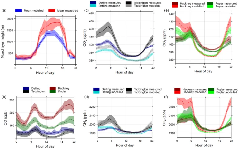
Figure 3. Mean diurnal cycles of (a) modelled (blue) and measured (red) boundary layer height and measured mean mixing layer height at North Kensington based on the spectral correction method described in Sect. 2.5, (b) measured CO mole fractions at the rural (Detling, blue), suburban (Teddington, black), and urban sites (Hackney, red; Poplar, green), (c) modelled (light shade) and measured (dark shade) CO2mole fractions at the rural (Detling, blue) and suburban (Teddington, black) sites, (d) modelled and measured (dark shade) CH4mole

fractions at the rural (Detling, blue) and suburban (Teddington, black) sites (d) modelled (light shade) and measured (dark shade) CO2mole

fractions at the urban (Hackney, red; Poplar, green) sites and (f) modelled and measured CH4mole fractions at the urban (Hackney, red;

Poplar, green) sites. June data are excluded due to unavailability of data during this period at Detling. Shading represents an estimate of the 95 % confidence interval in the mean, related to the limitation of the sampling of the daily values at a given hour, assuming these values are independent (based on the division of 2 times their temporal standard deviation by the square root of the number of values).

the model has a 2 km horizontal resolution. Figure 2 shows wind roses at Hackney and Poplar for measured CO and CO2,

and modelled CO2, alongside aerial images of the site

loca-tions. To reduce the influence of boundary layer variation on the measured and modelled mole fractions, and to anticipate the data selection on which the study will focus, we include measured and modelled data for the afternoon period only (see Sect. 3.2).

At Hackney there is an increase in measured CO and CO2

mole fractions during periods of south-easterly wind (Fig. 2a and b). A busy roundabout is located approximately 10 m to the south-east of the Hackney site with an A-road run-ning from north to south to the east of the sensor location (Fig. 2d). There is no increase for south-easterly winds when analysing modelled CO2 (Fig. 2c), suggesting that the

ob-served increase in the measurements could be related to the roundabout whose specific influence cannot be represented at the 2 km resolution in the model.

At Poplar, the measured CO and CO2is more uniform than

at Hackney (Figs. 2e and f). It is still higher in the east, but there is no visible signature of the busy roads to the north and south of the site (Fig. 2h). The modelled CO2at Poplar

(Fig. 2h) is very similar to that of Hackney (Fig. 2c), which can be explained by the proximity between the two corre-sponding model grid cells (Fig. 1). This supports the earlier assumption that the high mole fractions obtained at Hack-ney for south-easterly winds are related to a local source. These analyses also raise a more general assumption that while the model simulates the signature of emissions at a rel-atively large scale (due to handling emissions and transport at 2 km resolution and with significant numerical diffusion) in the area of these 2 sites, there are likely local-scale unre-solved emissions strongly influencing observed CO2at both

urban sites.

At both urban sites the observed CH4wind roses are very

of the sites (data not shown); however, mole fractions are greater in magnitude at Poplar than at Hackney. Similarly to CO2, the model simulates lower CH4mole fractions than

ob-served, with a similar distribution at both sites. The stronger similarity between the wind roses at the two sites when considering CH4measurements than when considering CO2

measurements could be explained by the absence of strong CH4 local sources in the vicinity of the measurement sites.

The NAEI does not locate any major waste treatment facil-ity at less than 5 km from these sites and it assigns a level of emissions from the other sectors (which are characterised by diffuse sources in the inventory) for this vicinity that is similar to the general level of CH4emissions in the London

urban area. Local CH4leaks from the gas distribution could

occur and impact the measurements, but this analysis does not highlight such local sources.

Despite the potential influence of local sources that are un-resolved by the transport model, we attempt, in the follow-ing sections, to understand and decompose the large discrep-ancies between the model and the measurements illustrated in Fig. 2. The objective is to analyse whether one can iden-tify the discrepancies due to errors in the emissions at scales larger than 2 km × 2 km, which should give insights on the potential for applying atmospheric inversion.

3.2 CO2, CH4and mixing layer mean diurnal cycles

The mean observed and modelled diurnal cycles of the CO, CO2and CH4mole fractions at the four GHG measurement

sites and the mixing layer height at North Kensington (see Sect. 2.5) are presented in Fig. 3. The amplitude of the mean diurnal cycle in mixing layer height (Fig. 3a) is approxi-mately 1500 m, typical of summer convective conditions in an urban area (Barlow et al., 2014).

Observed CO2mole fractions at all sites follow a typical

mean diurnal cycle (Fig. 3) with maximum mole fractions in the early morning (approx. 05:00 UTC) and minimum mole fractions during the afternoon (approx. 15:00 UTC), which can be related to the typical variation in mixing height (Fig. 3a), and in vegetation CO2exchanges (with

photosyn-thesis and a CO2 sink during daytime but CO2 emissions

during night-time) during a daily cycle. The early morning peak in CO2mole fractions occurs on average an hour later at

the inner city sites (06:00 UTC) compared with the rural and suburban sites (05:00 UTC) as shown in Fig. 3c and e. This may be due to the signature of working-week urban emis-sions with a peak in traffic around 06:00 to 09:00 UTC. This is supported by large observed CO mole fractions at the ur-ban sites with substantial early morning and evening peaks (Fig. 3b). The peak in CH4measured mole fractions occurs

at around 06:00 UTC at all sites (Fig. 3d and f).

At all sites the model underestimates by 1 to 5 % (by 5 to 9 ppm for CO2 and by 13 to 29 ppb for CH4)the mean

observed CO2 and CH4 mole fraction during the afternoon

hours (12:00 to 17:00 UTC), with the highest biases at

Hack-ney for CO2and at Poplar for CH4(see the model–data

bi-ases for this period in Table 1). This underestimation is con-sistently larger than the confidence intervals for the aver-aging (associated with the limited time sampling) indicated throughout Fig. 3. The underestimation continues through-out the diurnal cycle at Detling and Teddington (Fig. 3c and d); however, at the urban sites (Fig. 3e and f), the night-time (00:00 to 05:00 UTC) CO2and CH4mole fractions are

con-siderably larger in the model than in the observations. This leads to excessively strong diurnal variations at the urban sites, with the exception of CH4at Poplar (Fig. 3f).

On average, mixing layer height is underestimated in the model at North Kensington by approximately 13 % (46 m) of the equivalent lidar measurement during the night and 33 % (583 m) during the afternoon (Fig. 3a). There is a high daily variability in the mixing layer height model–lidar measurement discrepancies (with a 454 m SD in the 12:00– 17:00 UTC period and a 394 m SD in the 00:00 to 05:00 UTC period), and thus this underestimation is not systematic (see Sect. 3.4). However, this may still explain the overestima-tion of mole fracoverestima-tions at the urban sites during night-time but cannot explain the underestimation of CO2 and CH4 mole

fractions during the afternoon.

Accurate modelling of the boundary layer height in me-teorological models is an on-going concern, particularly in urban areas (Gerbig et al., 2008; Lac et al., 2013) and de-scription of nocturnal stratification is weak in atmospheric transport models (Geels et al., 2007). During the night there can be a considerable urban heat island in London as shown for North Kensington and rural Chilbolton by Bohnensten-gel et al. (2015). The model used in our study does not cur-rently have an urban land-surface scheme capable of repro-ducing the urban heat island effects on atmospheric transport (Sect. 2.4). This may explain the different sign of the model– data discrepancies during night-time between the urban sites and the other sites. We thus restrict the remaining analyses in this paper to the period between 12:00 and 17:00 UTC, wherein we can expect the boundary layer to be well devel-oped, to have a stable height and to exert minimum influence on the variations in gas mole fractions (Geels et al., 2007; Göckede et al., 2010).

3.3 Comparison between modelled and measured winds

This section focuses on the horizontal wind, which is a crit-ical driver of day-to-day variations in GHG mole fractions. We aim to validate the model wind forcing through com-parison with meteorological sites described in Sect. 2.5. The analyses (using hourly data) of measured and modelled wind are restricted to between 12:00 and 17:00 UTC because all further GHG analyses are focused on this afternoon period (Sect. 3.2).

At East Malling, on average, the model underestimates wind speed by 0.50 m s−1 (12 % of the observation mean)

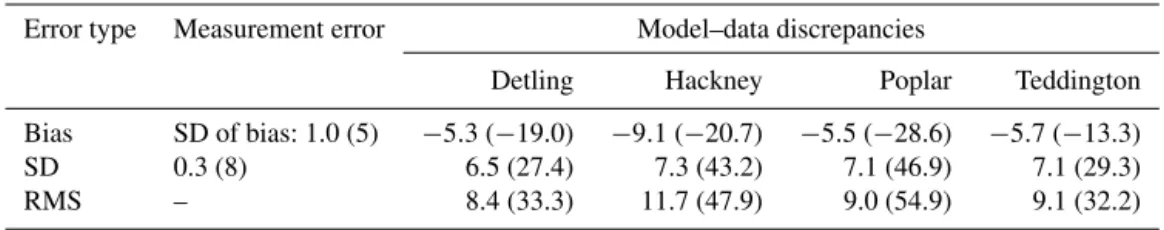
Table 1. Summary of systematic and random errors of hourly measurements (see Sect. 2.3) and of the hourly model–data discrepancies using data between 12:00 and 17:00 UTC during July to September 2012. Values are given for CO2(CH4in brackets) in parts per million (ppm)

and parts per billion (ppb) for CH4. SD denotes standard deviation; RMS denotes root mean square.

Error type Measurement error Model–data discrepancies

Detling Hackney Poplar Teddington

Bias SD of bias: 1.0 (5) −5.3 (−19.0) −9.1 (−20.7) −5.5 (−28.6) −5.7 (−13.3)

SD 0.3 (8) 6.5 (27.4) 7.3 (43.2) 7.1 (46.9) 7.1 (29.3)

RMS – 8.4 (33.3) 11.7 (47.9) 9.0 (54.9) 9.1 (32.2)

and wind direction by 6.90◦(defining positive angles clock-wise hereafter). The RMS of the hourly model–data discrep-ancies is 1.10 m s−1for wind speed and 26◦for wind direc-tion. At Heathrow Airport, there is an average positive bias of 0.37 m s−1(7 % of observation mean) and 5◦for wind speed and direction respectively (RMS model–data discrepancies of 1.27 m s−1and 2.24◦for wind speed and direction respec-tively). Some of this discrepancy may arise from the neces-sity of comparing the 25–50 m average wind data from the model to the 10 m height measurements at the Heathrow me-teorological station.

It is highly difficult to translate such statistics of the errors on the wind into typical errors on the simulation of the GHG concentrations at the GHG measurement sites since there is a complex relationship between them, which strongly depends on the specification of the local to remote emissions, and on the spatial distribution of the errors in the meteorologi-cal parameters or in these emission estimates at the lometeorologi-cal to larger scales. The overestimation of the wind speed in the urban area, unlike the underestimation of the mixing layer height, could partly explain the underestimation of the after-noon GHG concentrations at the urban sites since it should lead, on average, to an underestimation of the signature of the urban emissions. However, such an impact of the 7 % over-estimation of the urban wind speed cannot explain, by itself, the 5 to 9 ppm (21 to 29 ppb) underestimation of the urban CO2 (CH4)afternoon concentrations since the average

dif-ferences between the urban and rural or suburban concentra-tions during the afternoon do not exceed 10 ppm and 30 ppb according to both the model and the measurements (Fig. 3).

Lac et al. (2013) employed the Meso-NH meteorologi-cal model at 2 km horizontal resolution with an urban sface scheme that models specific energy fluxes between ur-ban areas and the atmosphere. Their modelled meteorology was compared with hourly meteorological measurements in the Paris region. They showed a typical bias of 0.8 m s−1 for wind speed and 20◦ for wind direction, which is larger than the agreement obtained here with the ECMWF winds driving CHIMERE at a native resolution of 15 km. Nehrkorn et al. (2013) found a wind speed bias of between −1 and 2.5 m s−1and RMS of between 1 and 4 m s−1when compar-ing the Weather Research and Forecastcompar-ing (WRF) model at 1.33 km resolution over Salt Lake City, US, with an urban

land-surface scheme, to local hourly wind measurements. Therefore, the choice of a 15 km wind field to force the CHIMERE transport model over London does not seem to raise typical wind errors larger than when using a state-of-the-art meteorological model at typically 1 to 3 km resolu-tion.

3.4 Daily CO2and CH4mole fractions during the

mid-afternoon

The average CO2and CH4mole fractions for the afternoon

of each day throughout the analysis period are presented in Figs. 4 and 5. Some data have been excluded from these analyses; we ignore hereafter, at a given site, any hour dur-ing which either modelled or measured data were not avail-able. We have also excluded data from 29 August and 23 to 24 September since the model simulated very large GHG peaks on these days which do not occur in the data. Data from June have been excluded from the statistical analysis to maintain comparability with Detling at which data were not available during this month.

According to both the measurements and the model, there is an increase in both the mean value (typically by 7 ppm and 26 ppb according to the measurements) and variability (typ-ically by 1 ppm and 16 ppb according to the measurements) of CO2and CH4mole fractions, from the rural and suburban

Detling and Teddington sites (Figs. 4a, d, 5a and d) to the urban sites Hackney and Poplar (Figs. 4b, c, 5b and c). This can be explained by their relative distance to the main area of anthropogenic emission in the centre of London (Fig. 1) and due to the location of Teddington (Detling) to the south-west (south-east) of the London area, while the dominant wind directions are from the west. According to the model, in gen-eral, modelled CO2is lower than the signature of the

Mon-itoring the Atmospheric Composition and Climate Interim Implementation (MACC-II) boundary conditions (BC-CO2

in Fig. 4) at Detling and Teddington (by ∼ 3 ppm on average) since the negative signature of the CO2NEE is larger than the

positive signature of the anthropogenic emissions between the model boundaries and these sites (see Fig. 4a and d). The London emissions between Detling or Teddington and Hack-ney or Poplar compensate for this decrease (see Fig. 4b and c) in such a way that CO2at Hackney and Poplar is

gener-Figure 4. Time series of averages for the afternoon period (12:00 to 17:00 UTC) each day of modelled CO2mole fractions (red), measured

CO2mole fractions (blue), modelled signature of the CO2boundary condition mole fractions from MACC-II (BC-CO2, black), the

mod-elled signature of the CO2fossil fuel emissions added to that of the boundary conditions (BC-CO2+FF-CO2, orange) and the modelled

signature of the CO2NEE added to that of the boundary conditions (BC-CO2+BIO-CO2, green) at (a) Detling, (b) Hackney, (c) Poplar and

(d) Teddington.

ally similar to BC-CO2(with less than 1 ppm difference on

average over July–August), except in September, when it is higher (by ∼ 5 ppm on average) because of the NEE being weaker in this month than during the previous months. Fur-thermore, the NEE and the anthropogenic emissions do not strongly alter the CO2variability from the boundary

condi-tions and the correlation (R value) between the variacondi-tions in modelled hourly CO2 and those of hourly BC-CO2is high

(between 0.75 and 0.85, depending on the site) even at urban sites. The modelled CH4 time series, which uses a constant

value at the boundaries, cannot show such a dependency on the model boundary conditions (Fig. 5).

Statistical comparisons between modelled and measured hourly CO2 and CH4 mole fractions are given in Table 1.

While the magnitude of the SD of the model–data discrepan-cies is similar to that of the bias for CO2, it is far larger than

the bias for CH4. The RMS of CO2model–data

discrepan-cies is highest at Hackney (12 ppm) but similar at the other three sites (8 to 9 ppm, Table 1). Higher RMS of CH4model–

data discrepancies are found at Poplar and Hackney (48 and 55 ppb) than at Teddington and Detling (32 and 33 ppb) (Ta-ble 1). The model–data discrepancies are substantially larger than measurement errors for both CO2 and CH4 (Table 1)

so we can exclude measurement error as a key source of the discrepancies. The discrepancies should thus mainly be as-sociated with representation errors (Sect. 3.1), transport

er-rors (Sect. 3.3), erer-rors in the domain boundary conditions and in the prescribed fluxes within the domain and outside the London area, or with errors in the emissions prescribed in the London area (based on NAEI data; see Sect. 2.1). The model–data CO2 or CH4 hourly discrepancies at the

urban sites during the afternoon are not significantly corre-lated (R values are between 0 and 0.2 for all cases) with the mixing layer height model–lidar measurement discrepan-cies at North Kensington (Sect. 3.2) or with the wind speed or direction model–data discrepancies at Heathrow Airport (Sect. 3.3).

Model–data correlations are significantly higher for hourly CH4(R values between 0.4 and 0.6, depending on the sites)

than for hourly CO2(between 0. and 0.1). However, the

am-plitude of the variations in hourly CH4 is strongly different

between the model (whose SD is of 15.5 to 18.5 ppb depend-ing on the sites) and the measurements (whose SD is of 32.8 to 51.5 ppb), which explains the very large model–data dis-crepancies given in Table 1. The potential impact of local CH4 sources near the urban sites (see Sect. 3.1) cannot

ex-plain that these discrepancies are very high at Teddington and Detling even though they can explain that they are signif-icantly larger at Hackney and Poplar. This suggests that the actual CH4conditions on the boundaries of the modelling

mea-sured CH4, as for CO2, but we miss it through the use of

constant CH4boundary conditions in the model.

3.5 CO2and CH4gradients between pairs of sites

An increasing number of studies on the atmospheric moni-toring of the city emissions focus on analysing and assimi-lating measurement gradients (Bréon et al., 2015; McKain et al., 2015; Turnbull et al., 2015; Wu et al., 2015; Staufer et al., 2016) rather than measurements at individual sites since it reduces the influence of the GHG fluxes that are outside the city of interest (of the model boundary conditions and of the fluxes that are outside the city but within the model do-main when analysing model simulations). This approach as-sumes that such an influence has a large spatial and temporal scale and is therefore similar for different measurement sites in and around the city (Bréon et al., 2015). Here, the strong influence of boundary conditions on the modelled CO2, and

the potential issue raised by using a constant boundary con-dition for the CH4simulations, leads us to assume that

uncer-tainties in both of the CO2or CH4boundary conditions can

explain a large part of the substantial discrepancies between observed and modelled GHGs that are diagnosed at the four measurement sites. We thus analyse the CO2or CH4

gradi-ent between the urban sites and the rural or suburban sites. Because of this computation, the rural and suburban sites are called hereafter “reference sites”. This analysis requires data at both the urban and the reference sites for a given hour and thus adds a new criterion to the data time selec-tion already described and applied in Sect. 3.4. The gradients are henceforth described as follows: Hackney and Detling (HAC–DET), Hackney and Teddington (HAC–TED), Poplar and Detling (POP–DET) and Poplar and Teddington (POP– TED).

Figure 6 presents the daily afternoon mean gradients of measured and modelled CO2and CH4mole fractions (1CO2

and 1CH4)alongside the daily afternoon mean gradient of

modelled fossil fuel CO2 (FF-CO2)and NEE (BIO-CO2)

components (1FF-CO2 and 1BIO-CO2) from the model

simulation. One can see from Fig. 6 that the modelled 1CO2

closely tracks modelled 1FF-CO2(with R values of 0.80–

0.95 depending on the selected pair of sites), while 1BIO-CO2(the average of which is smaller than 0.9 ppm in

abso-lute value between all pairs of sites) and the influence of the boundary conditions on these gradients (the average of which is smaller than 0.1 ppm in absolute value between all pairs of sites) are relatively small, compared with 1FF-CO2,

partic-ularly when Teddington is used as the reference site (Fig. 6). This strongly supports the assumption that the signature of boundary conditions and fluxes outside the London area op-erates on a large spatial and temporal scale and is therefore similar between different sites within the London area, even though this cannot be directly verified from the measure-ments. We thus expect that both the modelled and measured gradients between the urban and the reference sites bear a

clear signature of the anthropogenic emissions from the Lon-don area.

The largest hourly 1CO2are observed on the HAC–DET

gradient with a mean (±SD) of 8.2 ± 5.3 ppm. The hourly POP–DET gradients have a mean (±SD) of 5.6 ± 4.6 ppm. These are much larger than the gradients observed by Rigby et al. (2008) between an 87 m tower in central London at less than 11 km from Hackney and Poplar and a rural location at less than 15 km from Teddington.

The bias, SD and consequently RMS of the model–data discrepancies between modelled and measured gradients of both CO2 and CH4 (Table 2) are much reduced compared

with the same metrics at individual urban sites (Table 1). The RMS of the model–data discrepancies is roughly halved for 1CO2 compared with CO2at a single urban site (from 9.0

or 11.7 ppm for the urban sites to 3.6–6.3 ppm for the gra-dients depending on the corresponding pairs of sites). There is also a small improvement in correlation between observed and modelled 1CO2compared with correlation between

ob-served and modelled CO2at individual urban sites (from

be-tween 0.02 and 0.13 to bebe-tween 0.20 and 0.35), but model– data correlations for 1CH4are reduced compared with those

for CH4at the individual urban sites (from between 0.42 and

0.58 to between 0.20 and 0.30).

The measurements at each site are affected by a constant calibration bias (see Sect. 2.3); therefore, the decrease in model–data biases after the gradient computation partially comes from the cancellation of this systematic error. How-ever, this systematic error (typically ±1 ppm and ±5 ppb for CO2 and CH4 respectively; Table 1) is much smaller than

the difference between the model–data biases when consid-ering the analysis of mole fractions at individual sites (Ta-ble 1) and those when considering gradients between these sites (Table 2). Furthermore, the random measurement error should be larger for gradients than at individual sites (since the SD of the measurement error for the difference between two data at individual sites is the RSS of the SD of the inde-pendent measurement errors for these data). Therefore, the main driver of the strong decrease in model–data discrepan-cies when analysing gradients instead of mole fractions at individual sites should be the strong reduction of the large scale errors from the boundary conditions and remote fluxes. The random component of the measurement errors should be uncorrelated between different sites, and thus the SD of the gradient measurement error should be

√

2 times the SD of the measurement error at individual sites. Therefore, the gra-dient measurement error should remain much smaller (typi-cally equal to 0.4 ppm and 11 ppb for CO2and CH4

respec-tively) than the gradient model–data discrepancies (Table 2). The gradient model–data discrepancies should thus mainly be related to model (transport and representation) errors and errors in the estimate of fluxes in the London area, unless a significant influence of the remote fluxes remains in the mea-sured gradients even though this section has shown that such an influence is negligible in the modelled gradients.

Figure 5. Time series of averages for the afternoon period (12:00 to 17:00 UTC) each day of measured CH₄mole fractions (blue), modelled CH4mole fractions (red) and the constant signature of the modelled CH4boundary conditions (BC-CH4, black) at (a) Detling, (b) Hackney,

(c) Poplar and (d) Teddington.

Table 2. Summary of systematic and random errors of hourly measured gradients (see Sect. 3.5, the standard deviation of the measurement error for gradients is computed as

√

2 times the value of Table 1, assuming null correlation of this error between different sites) and of the hourly gradient model–data discrepancies using data between 12:00 and 17:00 UTC during July to September 2012. Values are given for 1CO2(1CH4in brackets) in parts per million (ppm) and parts per billion (ppb) for CH4. The two last columns present discrepancies

for afternoon gradients to Teddington wherein Heathrow measured wind direction places Teddington upwind of each urban site (for angles between the wind direction and the direction between Teddington and a given urban site smaller than 20◦, see Sect. 3.6). SD denotes standard deviation; RMS denotes root mean square.

Gradient measurement error All afternoon discrepancies Teddington upwind

discrepancies only

HAC–DET POP–DET HAC–TED POP–TED HAC–TED POP–TED

Bias SD of bias: 0.0 (0) −3.8 (−2.6) −0.2 (−9.7) −2.9 (−7.1) 0.6 (−16.1) −1.4 (−3.5) 1.7 (−10.8)

SD 0.4 (11) 5.1 (34.4) 4.4 (36.6) 4.2 (28.3) 3.6 (32.2) 2.9 (14.5) 3.4 (11.0)

RMS – 6.3 (34.4) 5.1 (29.2) 4.4 (37.8) 3.6 (36.0) 3.2 (14.8) 3.7 (15.3)

3.6 CO2and CH4gradients with wind direction

filtering

Figure 6 shows that the fit between the modelled 1CO2

and 1FF-CO2 is better for gradients to Teddington than

to Detling. Potential explanations could be that Teddington is far closer to London’s centre than Detling (Fig. 1), and that Teddington is more frequently upwind of the city than Detling. The signature of fluxes outside the urban area can be assumed to be more homogeneous along the wind di-rection than over the whole urban area (Bréon et al., 2015;

Staufer et al., 2016), in particular for the measurements (for the model, the boundary conditions and fluxes outside Lon-don are prescribed with relatively coarse resolution products, see Sect. 2.4; so this signature is homogeneous over larger spatial scales in the model than in the measurements). Bréon et al. (2015) decreased the signature of the fluxes outside the Paris urban area by considering gradients between two sites along the wind direction rather than by considering all gradi-ents irrespective of the wind condition. Applying this general concept to our study, we expect the gradients to Tedding-ton to be representative of the London urban emissions more

Figure 6. Time series of averages for the afternoon period (12:00 to 17:00 UTC) each day of measured 1CO2(blue), modelled 1CO2(red),

modelled signature of the fossil fuel CO2emissions (1FF-CO2)(black) and modelled signature of the CO2 NEE (1BIO-CO2)(green)

between (a) Hackney and Detling, (b) Hackney and Teddington, (c) Poplar and Detling and (d) Poplar and Teddington. Time series of averages for the afternoon period (12:00 to 17:00 UTC) of measured (blue) or modelled (red) 1CH4between (e) Hackney and Detling,

(f) Hackney and Teddington, (g) Poplar and Detling, and (h) Poplar and Teddington. Vertical pink lines indicate days during which at least one hourly afternoon wind direction is within a ±20◦range around the direct line from the reference site to the urban site according to the wind measurements at Heathrow (if the reference site is Teddington) or East Malling (if the reference site is Detling).

often than the gradients to Detling. Measured gradients cal-culated without considering the wind direction, particularly gradients to Detling, could retain a significant influence of the boundary conditions and fluxes outside the London area (even though this does not occur in the model). In extreme cases, the signature of remote fluxes can be far lower at the urban sites than at Detling (e.g. if Detling, unlike the urban

sites, sees anthropogenic emissions from the continent) so that the signature of the anthropogenic emissions at the ur-ban sites could not compensate for it; this would explain why the measured gradients sometimes reach negative values (e.g. −20.9 ppm for CO2 on 9 September, while the wind blows

from the south-south-west) even though they were computed to isolate the signature of the London emissions (Fig. 6).