HAL Id: inserm-00664028
https://www.hal.inserm.fr/inserm-00664028
Submitted on 24 Feb 2012HAL is a multi-disciplinary open access
archive for the deposit and dissemination of sci-entific research documents, whether they are pub-lished or not. The documents may come from teaching and research institutions in France or abroad, or from public or private research centers.
L’archive ouverte pluridisciplinaire HAL, est destinée au dépôt et à la diffusion de documents scientifiques de niveau recherche, publiés ou non, émanant des établissements d’enseignement et de recherche français ou étrangers, des laboratoires publics ou privés.
Recording of fast activity at the onset of partial seizures:
Depth EEG vs. scalp EEG.
Délphine Cosandier-Rimélé, Fabrice Bartolomei, Isabelle Merlet, Patrick
Chauvel, Fabrice Wendling
To cite this version:
Délphine Cosandier-Rimélé, Fabrice Bartolomei, Isabelle Merlet, Patrick Chauvel, Fabrice Wendling. Recording of fast activity at the onset of partial seizures: Depth EEG vs. scalp EEG.. NeuroImage, Elsevier, 2012, 59 (4), pp.3474-87. �10.1016/j.neuroimage.2011.11.045�. �inserm-00664028�
Recording of fast activity
1
at the onset of partial seizures:
2
depth EEG vs. scalp EEG
3
4
D. Cosandier-Rimélé 1, F. Bartolomei 2,3,4, I. Merlet 5,6, P. Chauvel 2,3,4, F. Wendling 5,6
5
6
7
1 Bernstein Center Freiburg, University of Freiburg, Freiburg, Germany
8
2 INSERM, U751, Laboratoire de Neurophysiologie et Neuropsychologie, Marseille, France
9
3 Université de la Méditerranée, Faculté de Médecine, Marseille, France
10
4 CHU La Timone, Service de Neurophysiologie Clinique, AP-HM, Marseille, France
11
5 INSERM, U642, Laboratoire Traitement du Signal et de l'Image, Rennes, France
12
6 Université de Rennes 1, LTSI, Rennes, France
13
14
15
16
Correspondence:17
Fabrice Wendling18
LTSI – INSERM U642
19
Université de Rennes 1
20
Campus de Beaulieu, Bât. 22
21
35042 Rennes Cedex, France
22
Email: fabrice.wendling@univ-rennes1.fr
23
24
Abstract
1
Rapid discharges (25-80 Hz), a characteristic EEG pattern often recorded at seizure onset in
2
partial epilepsies, are often considered as electrophysiological signatures of the epileptogenic
3
zone. While the recording of rapid discharges from intracranial electrodes has long been
4
established, their observation from the scalp is challenging. The prevailing view is that rapid
5
discharges cannot be seen clearly (or at all) in scalp EEG because they have low signal-to-noise
6
ratio. To date, however, no studies have investigated the ‘observability’ of rapid discharges, i.e.
7
under what conditions and to what extent they can be visible in recorded EEG signals. Here, we
8
used a model-based approach to examine the impact of several factors (distance to sources, skull
9
conductivity, source area, source synchrony, and background activity) on the observability of
10
rapid discharges in simultaneously simulated depth EEG and scalp EEG signals. In our
11
simulations, the rapid discharge was clearly present in depth EEG signals but mostly almost not
12
visible in scalp EEG signals. We identified some of the factors that may limit the observability
13
of the rapid discharge on the scalp. Notably, surrounding background activity was found to be
14
the most critical factor. The findings are discussed in relation to the presurgical evaluation of
15
epilepsy.16
17
Keywords:18
Rapid discharges, observability, depth EEG, scalp EEG, computer simulations, epilepsy.
19
20
1. Introduction
1
Seizure onset in partial epilepsy is often characterized by the appearance of a sustained
low-2
voltage fast activity (typically in the beta-gamma range, i.e. 25-80 Hz), also referred to as a
3
‘rapid discharge’. Rapid discharges are often considered as electrophysiological signatures of
4
the ‘epileptogenic zone’, i.e. the brain region(s) involved in the generation of seizures (Bancaud
5
et al., 1965; Fisher et al., 1992; Wendling et al., 2003; Bartolomei et al., 2008). Furthermore,
6
from a clinical viewpoint, surgical prognosis has been found to be related to the removal of
7
brain areas generating rapid discharges (Alarcón et al., 1995; Lee at al., 2000; Wetjen et al.,
8
2009; Bartolomei et al., 2010). Investigations of rapid discharges are therefore of paramount
9
importance in the presurgical evaluation of patients with drug-resistant partial epilepsy, as they
10
could lead to better identification of the epileptogenic zone.
11
The recording of rapid discharges from intracranial (subdural and depth) electrodes is now
12
well established, and several studies have been dedicated to the investigation of the spatial,
13
spectral, and temporal features of rapid discharges in intracranial EEG signals (Allen et al.,
14
1992; Fisher et al., 1992; Alarcón et al., 1995; Wendling et al., 2003). By contrast, the
15
observation of rapid discharges in scalp EEG is challenging. Several studies have investigated
16
the scalp EEG correlates of intracranial fast onset activities. Most reported that seizure onset is
17
correlated with EEG attenuation (‘flattening’) or no detectable scalp EEG changes (Gastaut and
18
Broughton, 1972; Pacia and Ebersole, 1997), and only very few have actually reported the
19
presence of rapid discharges (Worrell et al., 2002).
20
The common view is that rapid discharges cannot be seen clearly (or at all) in scalp EEG
21
because they suffer from a low signal-to-noise ratio and also are often obscured by muscle
22
artifacts. To date, however, no studies have investigated the ‘observability’ of rapid discharges,
23
i.e. under what conditions and to what extent they can be visible in recorded EEG signals. The
24
observability of any specific EEG activity depends on the complex interaction of several factors
25
such as the spatiotemporal configuration of the sources, the distance from the recording
26
electrode to the sources, the background activity, and the electrical properties of the conductive
media in the head. A thorough understanding of the biophysics of EEG measurements therefore
1
requires isolating the contribution of each of these factors. Such an investigation is hardly
2
possible to perform experimentally. However, it can be conducted with computer models, which
3
provide a unique opportunity to study the relative influence of individual parameters as well as
4
their interrelationships.
5
We recently proposed a neurophysiology-inspired computational model that allows for the
6
investigation of the relationship between the activation of brain sources and the corresponding
7
EEG signals (Cosandier-Rimélé et al., 2007, 2008). This model combines an accurate
8
description of the intracerebral sources (accounting for both the geometry of cortical dipole
9
layers and the neuronal activities) with a biophysically relevant description of the transmission
10
of source activities from the cerebral cortex to the recording electrodes. In previous studies, we
11
used the model to study the influence of source-related parameters (location, area, geometry,
12
and synchrony) on the properties of simulated signals during interictal spike activity, and
13
established quantitative relations between these parameters and the observability of spikes in
14
depth and scalp EEG signals (Cosandier-Rimélé et al., 2007, 2008).
15
In the present work, a similar model-based approach was used to investigate the impact of
16
different factors (source-to-sensor distance, skull conductivity, source area, source synchrony,
17
and background activity) on the contribution of rapid discharges to EEG signals. The objective
18
was to examine the conditions that facilitate or impair the recording of rapid discharges. To this
19
purpose, the EEG generation model has been adapted in order to produce fast activity as
20
observed at seizure onset in partial epilepsies. Then, the model was used to explore the specific
21
effects of each parameter on the observability of rapid discharges (as assessed by the ‘energy
22
ratio’ statistic) in simulated EEG signals. The investigation was conducted in simultaneously
23
simulated depth and scalp EEG signals, for comparative study of the sensitivity and specificity
24
of the two recording techniques.
25
26
27
2. Methods
1
2
2.1 Computational model of EEG signals
3
Our computational, generative model of EEG signals combines a neurophysiology-based model
4
for the simulation of neuronal activity in the cerebral cortex with a biophysically relevant
5
description of the transmission of electric fields from the cerebral cortex to the recording
6
electrodes.
7
8
2.1.1 Generation of neuronal activity
9
Cortical neuronal activity was simulated using a population-level modeling approach that
10
describes the average activity of neural ensembles, without explicit representation of individual
11
cell properties. Readers may refer to (Deco et al., 2008; Wendling and Chauvel, 2008) for recent
12
reviews and detailed information on population-level models, also referred to as ‘neural mass’
13
models.
14
In our model, a neuronal population consists of three interacting subpopulations: a
15
subpopulation of excitatory pyramidal cells and two subpopulations of inhibitory interneurons
16
mediating synaptic currents with either slow or fast synaptic kinetics (Fig. 1A). This model is a
17
modified version of the model proposed in (Wendling et al., 2002, 2005), initially developed for
18
hippocampus. This three-subpopulation model also complies with the neocortical cellular
19
organization, as the neocortex is mainly composed of excitatory pyramidal neurons and
20
inhibitory interneurons (Somogyi et al., 1998; Markram et al., 2004). In addition, there is
21
experimental evidence for the presence of both slow and fast forms of inhibition in neocortex,
22
which are mediated by two distinct subpopulations of interneurons (Benardo, 1994; Tamás et al.,
23
2003). The intrinsic connectivity parameters (average number of synaptic contacts between
24
pyramidal cells and inhibitory interneurons) have been changed according to anatomical data on
25
neocortical circuits (Markram et al., 2004). Moreover, in the present work, several neuronal
populations were considered and connected to each other (Jansen and Rit, 1995; Wendling et al.,
1
2000). All parameters and equations of the model are provided in the Appendix.
2
3
2.1.2 Calculation of electrical potentials
4
Simulated EEG signals were calculated by solving the so-called ‘EEG forward problem’, i.e. by
5
computing the electric field potentials for a given source configuration in the head volume
6
conductor. Our spatio-temporal source model and potential calculations have been described in
7
details elsewhere (Cosandier-Rimélé et al., 2007, 2008). Main assumptions and principles are
8
summarized hereafter.
9
10
Source model – The EEG sources were assumed to be the cortical pyramidal neurons (i.e.
11
activity in subcortical structures was not considered in the model). They were represented as
12
dipole layers distributed over the neocortex surface. The convoluted anatomy of the neocortex
13
was accounted for by using a triangular mesh of the cortical surface, obtained from the
14
segmentation of 3D resonance magnetic images. In this high resolution mesh (mean triangle
15
area of ~1 mm2), each mesh triangle was assumed to correspond to a distinct cortical neuronal
16
population. The electrical contribution of each population was represented by a current dipole
17
positioned at the barycenter of the corresponding mesh triangle and oriented perpendicular to its
18
surface. The magnitude of the moment of each dipole was proportional to the area of the mesh
19
triangle. Its time-course, which represents the time-varying dynamics of the associated
20
population, was provided by the output of the neuronal population model (summation of
21
postsynaptic potentials), as described above.
22
23
Potential calculation – Electric potentials were calculated at both scalp electrodes (scalp EEG)
24
and depth-electrode contacts (depth EEG). Calculations were performed in the quasistatic
25
approximation, i.e. we assumed that the activity of sources projected instantaneously (i.e. with
26
no time delays) onto recording electrodes (Plonsey and Heppner, 1967). On the one hand, scalp
27
EEG measurements are very sensitive to the geometrical and electrical properties of the head
tissues through which electric fields are transmitted. Scalp potential calculations were thus
1
performed in a realistically shaped head model obtained from the segmentation of 3D magnetic
2
resonance images. This model consisted of three electrically homogeneous compartments
3
representing the brain, the skull, and the scalp. The boundary element method (Hämäläinen and
4
Sarvas, 1989, Meijs et al., 1989) was used to compute the scalp potentials. On the other hand, in
5
intracerebral recordings, both sources and electrodes are located within the brain and therefore,
6
depth EEG measurements are mostly sensitive to the properties of the surrounding brain tissue.
7
In this particular case, forward calculations can be simplified by assuming the head is a
8
homogeneous brain region, i.e. omitting the skull and scalp compartments, and by considering it
9
as an infinite medium (Cosandier-Rimélé et al., 2007). The intracerebral potentials were thus
10
computed using the electrostatic potential formulation (Malmivuo and Plonsey, 1995).
11
12
2.1.3 Computer simulations
13
In this study, we assumed a ‘focal’ organization of the epileptogenic zone, i.e. epileptic activity
14
was generated by only one neocortical region (Aubert et al., 2009). The source of epileptic
15
activity was simulated by using a set of contiguous triangles on the cortical mesh, or ‘patch’
16
(Fig. 1C). Dipoles within the patch were assigned an epileptic time-course (fast activity), while
17
all other dipoles, outside the patch, were assigned a ‘normal’ time-course to simulate
18
surrounding background EEG activity. The two conditions (normal and epileptic) were obtained
19
from two different parameter settings (related to excitation and inhibition within a population)
20
in the neuronal population model (Fig. 1B). Specifically, the model generated a fast activity if
21
slow dendritic inhibition was decreased such that the populations of neurons became ‘more
22
excitable’, while keeping the capacity of generating fast inhibitory postsynaptic potentials, as
23
already shown in (Wendling et al., 2002, 2005). Model parameter values are provided in
24
Appendix (see Table 1).
25
From this extended cortical source model, the EEG signals were simulated simultaneously
26
on scalp electrodes as well as on depth-electrode contacts. Scalp potentials were computed at 32
27
positions on the scalp surface of the head model. They corresponded to a subset of 28 electrodes
of the 10/10 system, and 4 additional subtemporal electrodes (FT9, FT10, TP9, and TP10).
1
Intracerebral potentials were computed at 10 contact positions along a virtual depth electrode
2
orthogonally placed in the epileptic source (electrode entry point in the ‘middle’ of the cortical
3
patch). The depth-electrode contacts were represented as points spaced at 3.5 mm.
4
5
2.2 Model parameter sensitivity analysis
6
The observability of a given EEG activity depends on several factors that are related to the
7
source configuration and to volume conduction (i.e. conditions of the transmission of electric
8
fields from the sources to recording electrodes). In this work, we focused on three factors in the
9
former category (source area, source synchrony, and background activity), and two factors in
10
the latter category (source-to-sensor distance and skull conductivity). Five simulation scenarios
11
were thus designed, each one addressing the specific influence of one of these factors on the
12
observability of rapid discharges in depth and scalp EEG signals, comparatively. They are
13
detailed hereafter, along with a description of the model parameter under investigation in each
14
case.
15
Besides, the results of our sensitivity analysis may depend on the selected source location in
16
the brain. Indeed, the neocortex surface is highly convoluted and the particular location,
17
geometry, and ‘orientation’ of cortical sources with regard to the recording electrodes markedly
18
impact the measured potential distributions (Gloor, 1985). To take account of the influence of
19
these factors, and ensure we capture the general trends of the effects of investigated parameters,
20
all our simulations were performed for ten different positions of the epileptic cortical patch
(P1-21
P10, Fig. 1D). All ten positions were arbitrarily lateralized in left hemisphere.
22
23
2.2.1 Simulation scenario 1 – Effect of the source-to-sensor distance (parameter D)
24
It is acknowledged that the distance of the source to the measuring sensor influences the EEG
25
signal amplitude, since the potential falls off as a function of this distance. In this simulation
26
scenario, the impact of source-to-sensor distance (parameter D) on the observability of rapid
27
discharges was analyzed by comparing fast activities simulated at three recording sites, located
at three different distances from the source: the source itself (i.e. within the epileptic cortical
1
patch), depth-electrode contacts, and scalp electrodes. The activity of the epileptic patch was
2
approximated by summing the fast onset activities generated by neuronal populations within the
3
patch, weighted by the area of their corresponding cortical mesh triangle. The distance between
4
a measurement sensor and the epileptic cortical patch was computed as the mean Euclidean
5
distance from the sensor to all dipoles within the patch. Additionally, to ensure we isolate the
6
influence of distance from volume conductor modeling effects (related to the geometry and
7
electrical properties of the head model), both intracerebral and scalp forward calculations were
8
performed in an infinite homogeneous volume conductor (in contrast with the other four
9
simulation scenarios, in which scalp forward calculations were performed using the realistic
10
head model). The conductivity of the medium was set to 0.33 S/m (a commonly used value for
11
brain conductivity), and simulations were performed with a medium-sized (S=10 cm2),
12
moderately synchronized (K=K2) epileptic patch and surrounding background activity (!=1).
13
14
2.2.2 Simulation scenario 2 – Effect of the skull conductivity (parameter R)
15
It is well known that the skull has a very low conductivity relative to the other head
16
compartments. Because of its low conductivity, the skull strongly attenuates electric fields as
17
they flow through it. However, there is no consensus on the skull conductivity value and a wide
18
range of values have been reported (Rush and Driscoll, 1968; Oostendorp et al., 2000;
19
Gonçalves et al., 2003; Lai et al., 2005). The purpose of this simulation scenario was therefore
20
to investigate the impact of the skull conductivity value on the observability of rapid discharges
21
in scalp EEG signals. Depth EEG signals were not considered here. Scalp potentials were
22
computed using the realistic head model. The conductivities of the brain and the scalp were
23
assumed to be identical and were set to 0.33 S/m. The conductivity of the skull was expressed as
24
a fraction of the conductivity of the brain, and we defined a parameter R as the brain-to-skull
25
conductivity ratio. Four values of R were used for the simulations: 10, 20, 40 (the ‘standard’
26
value, used in the other four simulation scenarios) and 80, in accordance with the values
27
reported in the above-cited studies. In addition, to isolate the influence of conductivities from
the geometrical properties of the head model, we also considered R=1 (i.e. a head model
1
comprising three compartments with identical conductivities) as an ‘initial’ condition.
2
Simulations were performed with a medium-sized (S=10 cm2), moderately synchronized
3
(K=K2) epileptic cortical patch and surrounding background activity (!=1).
4
5
2.2.3 Simulation scenario 3 – Effect of the source synchrony (parameter K)
6
The synchronization of neuronal activity within the epileptic source is a crucial determinant of
7
the recorded EEG patterns. In our model, the source synchrony ‘level’ is controlled by using the
8
degree of coupling between the neuronal populations within the source. In the neuronal
9
population model, the connection from a given population i to a population j is characterized by
10
a parameter Kij that represents the coupling strength (Jansen and Rit, 1995; Wendling et al.,
11
2000). Based on recent findings on the coupling of neuronal fast activities (Wendling et al.,
12
2010), we assumed a ‘star-like’ network with unidirectional coupling (i.e. all populations are
13
connected to a center population), and all parameters Kij were set to a same value K. In this
14
simplistic connectivity model, the source synchrony level can be more easily controlled
15
compared to situations where random bi-directional coupling are present in the network. Its
16
influence can indeed be analyzed just by varying parameter K. Specifically, we used four
17
different values of K, to account for a null (K=0), low (K1), medium (K2), and high (K3) degree
18
of coupling between the neuronal populations. Both depth EEG and scalp EEG signals were
19
simulated, using a medium-sized (S=10 cm2) epileptic patch and surrounding background
20
activity (!=1).
21
22
2.2.4 Simulation scenario 4 – Effect of the source area (parameter S)
23
Determining the size of cortical sources of recorded epileptic EEG activities is a key issue in the
24
presurgical evaluation of epilepsy. To study the relationship between the spatial extent of the
25
source and the observability of rapid discharges in simulated EEG signals, we considered an
26
epileptic cortical patch with a varying surface area S. The surface area of a cortical patch was
27
defined as the sum of the surface areas of elementary mesh triangles included within the patch.
In simulations, the patch surface area S was varied from 1 to 30 cm2, by steps of 1 cm2 (Fig. 1E),
1
and both depth and scalp EEG signals were simulated. The two other source-related parameters
2
were kept constant (source synchrony level: K=K2, and background activity level: !=1).
3
4
2.2.5 Simulation scenario 5 – Effect of the background activity (parameter !)
5
In general, it is recognized that locally generated EEG activities tend to be overshadowed by the
6
background activity that is concurrently generated throughout the brain. In our model, the
7
simulated EEG results from the superposition of the potentials produced by the epileptic cortical
8
patch (generating fast activity) and those produced by the rest of the cortex (generating
9
background activity). The purpose of this simulation scenario was to examine the impact of the
10
amplitude of the background activity on the observability of rapid discharges in EEG signals.
11
To do so, we introduced a parameter ! that ‘weights’ the relative contribution of the background
12
activity to the simulated EEG. Depth and scalp EEG signals were simulated for all ! values
13
between 1 (‘control’ condition) and 0 (no background), with a step of 0.1. Simulations were
14
performed with a medium-sized (S=10 cm2), moderately synchronized (K=K2) epileptic patch.
15
16
2.3 Quantification of rapid discharges
17
The salient feature of rapid discharges is a redistribution of the energy of EEG signals from low
18
frequencies (in the delta-theta-alpha range) toward higher frequencies (typically, in the
beta-19
gamma range) (Bartolomei et al., 2008). In our model, the frequency range of fast activity is
20-20
25 Hz (in the high beta band), in contrast with frequencies of the background activity which are
21
mostly < 10 Hz (in delta and theta bands) (Fig. 1B). To study and illustrate the frequency
22
content of simulated EEG signals, we used the power spectral density (PSD, periodogram
23
method). Furthermore, we assessed the observability of rapid discharges in EEG signals by
24
computing the ratio of the energy of the EEG in two frequency bands: 0.1 to 8 Hz
(low-25
frequency energy, LE) and 18 to 30 Hz (high-frequency energy, HE). This ‘energy ratio’ (ER),
26
previously introduced in (Bartolomei et al., 2008), quantifies how much the rapid discharge
(HE) ‘emerges’ from the background (LE). It is computed from the signal spectral density "
1
(squared modulus of its Fourier transform):
2
ER = HE / LE, with LE =!
= ="
8 1 . 0)
(
f fdf
f
and HE =!
= ="
30 18)
(
f fdf
f
3
In practice, the ER values were computed as functions of time, over a sliding analysis
4
window. We denote by ER[n] the values computed at discrete time index n of the window
5
position. The window length was set to 4 s, and the sliding step to 0.25 s. The duration of the
6
simulations was 30s. The ER values were computed over the whole simulation duration (N=105
7
values). Then, for each simulated EEG signal si, we computed the mean ER (mERi) by
8
averaging the values over time:
9
mERi =
!
= N nN
11
ERi[n]
10
where i denotes the considered scalp electrode or depth-electrode contact.
11
Furthermore, in order to compare the results at the different patch locations, the mERi
12
values were normalized between 0 (no rapid discharge) and 1 (‘maximal’ rapid discharge). For
13
each patch location, mERi values were divided by the maximum value obtained in all
14
simulations. In 9 out of 10 cases, this maximum value was obtained in simulation scenario 1,
15
from the signal simulated at the level of the epileptic cortical source. In one case (P5), it was
16
obtained in simulation scenario 5, in the absence of background activity (!=0). In the sequel,
17
normalized mERi values are simply denoted by ‘mER values’.
18
19
2.4 Statistical analysis
20
Statistical analysis was performed to assess the effect of the investigated factors on the
21
observability of rapid discharges in simulated EEG signals. For each patch location, the mER
22
values were computed for each simulated depth and scalp EEG signal. The analysis then
23
focused on the EEG signals from the depth-electrode contact and the scalp electrode that are
24
closest to the epileptic cortical patch. We used box plots to compare the statistical distributions
25
of the mER values, as computed for different parameter settings. On each box, the central mark
is the median, the edges of the box are the 25th and 75th percentiles, the length of the whiskers
1
is 1.5 times the interquartile range, and any data point beyond the whiskers (outlier) is plotted
2
with a star. Furthermore, to assess the statistical significance of the differences in mER, we used
3
nonparametric Wilcoxon rank sum tests, with a significance level of 1%.
4
5
3. Results
6
7
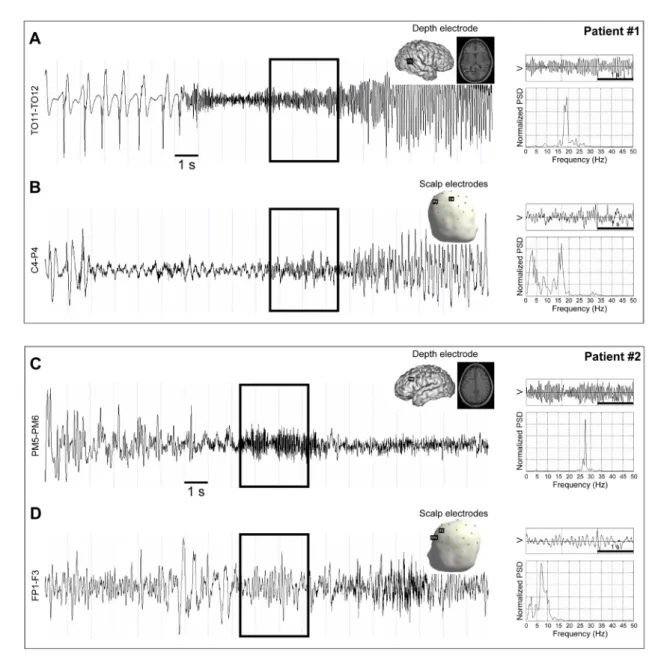
3.1 Examples of real rapid discharges
8
Before describing the results of the computer simulations, we present examples of real rapid
9
discharges recorded in two epileptic patients with drug-resistant epilepsy, during the transition
10
from normal to seizure activity. Patient #1 had focal cortical dysplasia located in the right lateral
11
occipital cortex and has been previously studies in a series of patients with focal epileptogenic
12
lesion (patient #6 in (Aubert et al. 2009)). Patient #2 had cryptogenic, left frontal lobe epilepsy.
13
Patient #1 illustrates the case of a rapid discharge that is visible both in depth EEG and in scalp
14
EEG recordings (Figs. 2A-B), while patient #2 illustrates a case of a rapid discharge that is
15
clearly present in depth EEG recordings but not visible in scalp EEG recordings (Figs. 2C-D).
16
In both cases, the rapid discharge is characterized by a narrowband activity (quasi-sinusoidal
17
signal), with a frequency between 15 and 20 Hz in patient #1 and between 25 and 30 Hz in
18
patient #2. When visible on the scalp (patient #1), the rapid discharge is highly contaminated
19
with low-frequency (<10 Hz) background activity. Simulated rapid discharges resemble real
20
ones in terms of morphology and spectral content, in both EEG modalities, as seen in simulation
21
examples shown below.
22
23
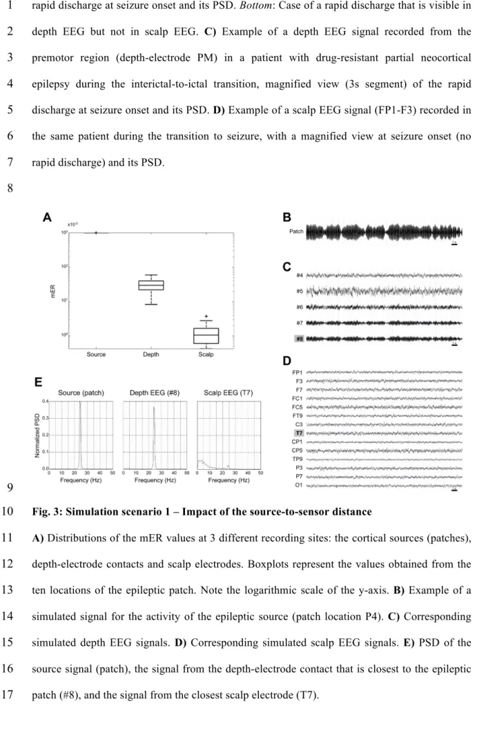
3.2 Simulation scenario 1 – Effect of the source-to-sensor distance
24
Results about the influence of the source-to-sensor distance (parameter D) are illustrated in Fig.
25
3. The observability of the rapid discharge greatly deteriorated as the recording site moved away
26
from the epileptic patch, as shown by a significant decrease in mER (Fig. 3A). The average
mER was 1.0 ± 0.0 (mean ± standard deviation) at the cortical sources, 32.39#10-3 ± 16.51#10-3
1
at depth-electrode contacts (with D values ranging from 9 to 10 mm), and 1.40#10-3 ± 1.08#10-3
2
at scalp electrodes (D from 22.3 to 31.7 mm). Visual inspection of simulated signals and their
3
spectra indicated that increasing the distance both decreased the high-frequency energy of the
4
simulated signals and increased the low-frequency energy (Figs. 3B-E). However, it appeared
5
that the increase in LE was much more important than the decrease in HE. Indeed, while the
6
rapid discharge was accompanied only by slight background activity in depth EEG signals, the
7
two activities were ‘blended’ in scalp EEG signals and the rapid discharge was little (or not)
8
visible in this case (Fig. 3E).
9
10
3.3 Simulation scenario 2 – Effect of the skull conductivity
11
Fig. 4 illustrates the effect of varying the brain-to-skull conductivity ratio (parameter R). The
12
mER was progressively reduced with increasing R (i.e. decreasing skull conductivity) (Fig. 4A).
13
However, there were no statistically significant differences in mER between the five tested
14
values of R. In addition, the mER values were already very low (<3#10-3) for R=1 (i.e. when the
15
brain, skull, and scalp had an equal conductivity). Visual inspection of simulated signals and
16
their spectra confirmed these observations and further revealed a marked attenuation of the
17
amplitude of the scalp EEG with increasing R (Fig. 4B).
18
19
3.4 Simulation scenario 3 – Effect of the source synchrony
20
Fig. 5 illustrates the effect of increasing the degree of coupling (parameter K) between the
21
neuronal populations within the epileptic patch. Fast activities were asynchronous for a null
22
coupling and became more synchronized as K increased. Thereby, the level of synchrony of the
23
source (as assessed by calculating the correlation coefficients (nonlinear regression coefficients
24
h2 (Pijn and Lopes da Silva, 1993; Wendling et al., 2001)) between population pairs within the
25
patch) increased with increasing K (Figs. 5A-B). At the level of the electrodes, the observability
26
of the rapid discharge was significantly improved when K was increased. In the absence of
coupling (K=0), the mER values were very low in both depth and scalp EEG signals. In depth
1
EEG signals, the mER was drastically increased between K=0 and K=K1 (the average mER was
2
multiplied by ~16), and then the amount of increase became progressively smaller (Fig. 5D). In
3
scalp EEG, there was a more gradual increase in mER with increasing K (Fig. 5F). In both
4
modalities, however, the difference in mER was no longer significant between K=K2 and K=K3.
5
The range of variation in mER was much wider in depth EEG (average mER between 0.59#10-3
6
± 0.29#10-3 for K=0 and 51.41#10-3 ± 24.73#10-3 for K=K3) than in scalp EEG (between
7
0.25#10-3 ± 0.02#10-3 and 0.95#10-3 ± 0.44#10-3). Visual inspection of simulated signals and
8
their spectra showed that increasing the neuronal coupling within the epileptic patch resulted in
9
a marked increase in high-frequency energy of the simulated EEG. In contrast with depth EEG
10
signals where the rapid discharge was very visible from K=K1 onwards (Fig. 5C), in scalp EEG
11
signals, the rapid discharge mostly hardly emerged from background activity for K=K3 (Fig.
12
5E).
13
14
3.5 Simulation scenario 4 – Effect of the source area
15
Results about the effect of extending the source surface area (parameter S) are shown in Fig. 6.
16
In both depth and scalp EEG signals, the observability of the rapid discharge was significantly
17
improved as the epileptic patch got larger. However, the relation between the mER and S
18
appeared to be very different in the two modalities. In depth EEG, the amount of increase in
19
mER was greatest for small patch surface areas and rapidly leveled off (Fig. 6A). Indeed, for 7
20
out of the 10 patch locations, the mER reached a ‘plateau’ level at surface areas between 5 and
21
10 cm2. In scalp EEG, by contrast, there was a more gradual increase in mER with increasing S,
22
although with some variability in the slope of the relation between patch locations (Fig. 6B). In
23
addition, the range of variation in mER was narrower in scalp EEG (average mER between
24
0.27#10-3 ± 0.02#10-3 at S=1 cm2 and 2.26#10-3 ± 1.27#10-3 at S=30 cm2) than in depth EEG
25
(between 1.21#10-3 ± 1.27#10-3 and 77.23#10-3 ± 62.43#10-3). Visual inspection of simulated
26
signals and their spectra indicated that the rapid discharge was clearly visible for very small
27
surface areas of the epileptic patch (<3 cm2) in depth EEG signals (Fig. 6C) whereas, in scalp
EEG signals, it emerged from background activity only for large surface areas (>10 cm2) (Fig.
1
6D). For one epileptic patch (P4), the rapid discharge was never visible on the scalp, even for
2
S=30 cm2.
3
4
3.6 Simulation scenario 5 – Effect of the background activity
5
Fig. 7 shows the results about the effect of varying the background activity level (parameter !).
6
In both EEG modalities, the observability of the rapid discharge significantly deteriorated with
7
increasing background level. In the absence of background (!=0), the mER values were very
8
high (>0.85) and comparable for depth and scalp EEG signals. In the presence of background
9
(!>0), on the other hand, the relation between the mER and ! was found to be very different in
10
the two recording techniques. In scalp EEG, there was a drastic reduction in mER for small !
11
values (Fig. 7B). Indeed, the average mER was divided by ~100 between !=0 and !=0.2, and by
12
~500 between !=0 and !=0.5. By contrast, in depth EEG, the mER decreased more gradually
13
between !=0 and !=1, for all ten patch locations (Fig. 7A). In addition, the mER values
14
remained much higher for !=1 in depth EEG (32.39#10-3 ± 16.51#10-3) than in scalp EEG
15
(0.65#10-3 ± 0.26#10-3). Visual inspection of simulated signals and their spectra showed that, in
16
scalp EEG, the rapid discharge rapidly ‘blended’ with background activity and it became less
17
visible for middle values of ! already (Fig. 7D), while in depth EEG, the rapid discharge was
18
very clearly visible for all ! values (Fig. 7C).
19
20
4. Discussion
21
To our knowledge, this study is the first that uses computer simulations to quantitatively address
22
the influence of different factors on the observability of rapid discharges at seizure onset, in
23
depth EEG and scalp EEG signals comparatively. The main findings are discussed below, along
24
with the limitations of the present study and suggestions for future research.
25
26
4.1 Low observability of rapid discharges in scalp EEG
A first general result is that the mER values obtained in scalp EEG were significantly lower
1
than those in depth EEG (they differed by one or two orders of magnitude). Visual inspection of
2
simulated signals and their spectra indicated that in many cases, the rapid discharge could not be
3
seen clearly (or at all) in scalp EEG, while simultaneously it was very visible in depth EEG.
4
Therefore, our model results are in agreement with prevailing views and further suggest that the
5
situations where favorable conditions are met for observing rapid discharges in scalp EEG
6
remain much more specific as compared with depth EEG. In addition, it should be mentioned
7
that our computer simulations were conducted in a well-controlled framework, unlike real scalp
8
EEG recordings where signals are also contaminated by artifacts (eye movements, muscle, etc.)
9
that further hamper the observation of rapid discharges. Our results may therefore overestimate
10
the actual observability of rapid discharges in scalp EEG signals.
11
12
4.2 Minor contribution of the attenuating effect of the skull
13
When examining the attenuating effect of the skull (simulation scenario 2), our results indicated
14
that, as expected, decreasing skull conductivity reduced the observability of the rapid discharge
15
in simulated scalp EEG signals. However, the reduction in mER was very small and not
16
statistically significant. Moreover, very low mER values were also obtained with a conductive
17
skull. Altogether, these findings suggest that the low skull conductivity is only a minor factor in
18
the lack of observable rapid discharges in scalp EEG, which contradicts the prevailing view on
19
the importance of this factor.
20
Besides, it should be emphasized that the lack of observable scalp rapid discharges is only
21
due to voltage attenuation, and that the skull does not filter out high-frequency components of
22
brain activity, as it is sometimes said. Indeed, it has long been established that the quasistatic
23
approximation holds for the EEG, i.e. there is no time-lag between electrical potentials recorded
24
at any point in the head and the underlying source activity (Plonsey and Heppner, 1967). Under
25
these conditions, the transfer coefficients from any source in the brain to any measuring sensor
26
(the so-called ‘EEG lead field’) depend only on the volume conductor properties (geometry and
27
conductivities of the head tissues) and on the positions and orientations of the sources with
respect to sensors. Thus, the spectral content of the neuronal activity is not altered during its
1
transmission from the cerebral cortex to the scalp, and the skull hampers the recording of rapid
2
discharges only because its low conductivity attenuates an already small activity (Gotman,
3
2010).
4
5
4.3 Major impact of background activity and distance
6
In our simulations, the level of background activity appeared to be the most critical factor
7
impeding the observability of rapid discharges. For both EEG modalities, the most conspicuous
8
variations in mER were observed in simulation scenario 5, where we found that mER values
9
were very high (close to 1) in the absence of background activity and were markedly reduced
10
with increasing background level. The impact of background activity appeared to be particularly
11
dramatic in scalp EEG signals, where a slight increase in background level resulted in a drastic
12
decrease in mER. While the role of background activity in EEG analysis and interpretation has
13
been recognized, these findings further highlight the crucial importance of this factor.
14
As expected, results indicated that the depth EEG was less susceptible to background
15
activity than the scalp EEG. Depth electrodes can be in direct contact with or in close vicinity to
16
some sources, which provides higher sensitivity but smaller volume of sensitivity to the depth
17
EEG recording technique. An advantage of a more restricted volume of sensitivity is that it
18
reduces the amount of surrounding background activity captured by the electrodes. Depth EEG
19
therefore enables a more reliable measure of rapid discharges, provided the electrodes are
20
accurately positioned in the involved brain region(s). In contrast, scalp electrodes remain remote
21
from brain sources. Their volume of sensitivity is thus very large and they record ‘mixtures’ of
22
source activities from the entire brain. Rapid discharges are difficult to observe in scalp EEG
23
because they originate from a limited brain area and they are overshadowed by the background
24
activity that is concurrently generated throughout the brain.
25
Besides, it should be mentioned that in our model, the background EEG was produced by
26
concurrently active neuronal populations distributed over the whole cortical surface, and that
27
these populations were independent from each other (non-coupled neuronal population models).
This is unlike real background EEG, as brain connectivity (structural, functional, and effective)
1
induces correlations in activity between different brain regions (Sporns, 2010). The presence of
2
correlated activity would probably increase the relative contribution of the background to the
3
recorded EEG signal and thereby, even further overshadow the local rapid discharges. Our
4
results may therefore overestimate the actual observability of rapid discharges.
5
As far as the source-to-sensor distance is concerned, the results in simulation scenario 1
6
indicated a strong impact of this factor, as shown by the significant decrease in mER with
7
increasing distance. Interestingly, we found a greater effect on low-frequency energy (LE) than
8
on high-frequency energy (HE) of the simulated EEG, i.e. a much more important increase in
9
LE compared with the decrease in HE. This finding suggests that distance influences the
10
observation of rapid discharges in recorded signals through its impact on the volume of
11
sensitivity of the electrode which, in turn, affects the amount of background activity captured by
12
the electrode. This view is further supported by results in simulation scenario 5, which indicated
13
that in the absence of background activity, the mER values were similar at the three considered
14
recording sites (cortical source, depth electrode, and scalp electrode). One likely explanation of
15
this finding is the linear relationship that exists between the amplitude of a measured potential
16
and the inverse of the distance between the electrode and a dipole layer (Cosandier-Rimélé et al.,
17
2007). Indeed, we previously showed that potential attenuation in the dipole layer model was
18
inversely proportional to source-to-sensor distance. Under these conditions, changing the
19
distance is therefore roughly equivalent to multiplying the EEG voltage by a weighting
20
coefficient. Given the definition of the mER quantity (a ratio of energies), it is insensitive to
21
such voltage ‘scaling’.
22
23
4.4 Influence of the source area and source synchrony
24
Our results (simulation scenarios 3 and 4) showed that extension of the surface area of the
25
epileptic source and strengthening of neuronal coupling within the source were associated with
26
improved observability of rapid discharges in simulated EEG signals. These findings are
27
consistent with the well-known fact that only neuronal activities that are synchronous over
rather large cortical areas yield potentials that can be recorded in EEG, and most particularly in
1
scalp EEG (Abraham and Ajmone-Marsan, 1958; DeLucchi et al., 1962; Cooper et al., 1965;
2
Tao et al., 2005, 2007; Cosandier-Rimélé et al., 2007, 2008). Interestingly, it has been suggested
3
that rapid discharges at seizure onset may originate from small brain areas (Tao et al., 2007) and
4
may be transiently desynchronized (Wendling et al., 2003), two conditions that would
5
contribute to make their recording from the scalp less likely. As expected, our simulation results
6
revealed a high sensitivity of the depth EEG, in which rapid discharges could be observed from
7
smaller cortical areas and lower synchrony levels as compared to the scalp EEG. However,
8
results in simulation scenario 4 also showed that the observability of rapid discharges in depth
9
EEG signals was not much improved when increasing the source area beyond 5-10 cm2, which
10
could demonstrate the spatial restriction of the volume of sensitivity of depth electrodes. As far
11
as scalp EEG signals are concerned, our results showed that the impact of source area and
12
source synchrony was relatively limited, as indicated by narrow ranges of variation in mER
13
when compared to depth EEG signals. It is noteworthy, however, that in our simulations, rapid
14
discharges became visible in scalp EEG signals for extended source area (simulation scenario 4).
15
The results in simulation scenario 3, on the other hand, showed that enhanced source synchrony
16
was not able to fully compensate for the inherent ‘shadowing effect’ of the background activity.
17
Overall, our simulation results are thus in agreement with previous clinical observations
18
indicating that rapid discharges are often not visible at seizure onset in scalp EEG recordings.
19
Strikingly, however, several recent studies demonstrated that fast activities (>40 Hz) can be
20
readily observed from the scalp (Kobayashi et al., 2004, 2009; Wu et al., 2008;
Andrade-21
Valenca et al., 2011). To some extent, these findings contrast with those reported in our study.
22
The most likely explanation for this discrepancy is the difference in the spatial configuration of
23
sources. Indeed, several studies reported on fast activities recorded in scalp EEG in patients
24
with severe types of epileptic seizures, such as epileptic spasms (Kobayashi et al., 2004; Wu et
25
al., 2008) and tonic seizures (Kobayashi et al., 2009), which generally reflect bilateral
26
widespread brain generators. A broader distribution of fast activities would contribute to make
27
them more visible on scalp recordings. This is in agreement with our finding that rapid
discharges became more visible as the epileptic patch got larger (simulation scenario 4).
1
Interestingly, diffuse amplitude attenuation (‘flattening’) also may occur during these types of
2
seizures. This may relate to the situation where the level of surrounding background activity
3
was decreased in our simulations, a situation that was shown to improve the observability of
4
rapid discharges (simulation scenario 5). In addition, very recently, a study demonstrated that
5
fast activities can also be recorded in scalp EEG in patients with focal epilepsy
(Andrade-6
Valenca et al., 2011), a context that is more similar to that of our study. However, the authors
7
suggested that the patients presented a ‘network’ organization of the epileptogenic zone, i.e.
8
epileptic activity was generated by multiple brain regions. The synchronous activation of these
9
regions would broaden the distribution of fast activities and thereby, contribute to improve their
10
observability on scalp EEG. It is noteworthy that in our study, the patient with scalp-recorded
11
rapid discharges (patient #1) presented an epileptogenic zone that included at least the
temporo-12
occipital junction and the mesial temporal cortex (entorhinal cortex). Future studies with
13
simulations using multiple epileptic sources are required to specifically address the issue of the
14
observability of rapid discharges in the context of a network organization of the epileptogenic
15
zone.
16
Besides, a comment should be made about the reduction in EEG amplitude that may occur
17
at seizure onset. Although frequent, the ‘low-voltage’ aspect is not a constant feature of rapid
18
discharges, suggesting at least two different situations of altered synchronization. First, most of
19
the neuronal populations within the epileptic source would generate synchronous fast activity as
20
a result of ‘organized connectivity’, as chosen in this study for the sake of simplicity. In this
21
case, resulting EEG signals are characterized by an increase of amplitude, as verified in our
22
simulations (Fig. 5). Second, in an alternative situation, each population within the patch would
23
generate a fast activity but independently from the others, as a result of random connectivity
24
patterns (in which the synchronization level is known to be more difficult to control and
25
measure (Wendling et al., 2010)). In this situation, it is expected that the low temporal
26
correlation among individual activities would lead to a decrease of amplitude in EEG signals.
27
As mentioned above, in this study, we chose a simple connectivity model, in order to examine
the relation of a well-controlled and measurable synchronization level within the epileptic patch
1
to the presence of rapid discharges in resulting EEG signals. Dedicated studies are still to be
2
performed to analyze more specifically the influence of connectivity patterns on the
3
observability of rapid discharges. Nevertheless, it is acknowledged that the present connectivity
4
model, with induced increase in signal amplitude, increases the relative contribution of rapid
5
discharges in the mixture with background activity, and our results thus probably overestimate
6
the actual observability of rapid discharges in EEG signals.
7
8
4.5 Impact of the source topology
9
Results presented in this study were obtained from ten different positions of the epileptic
10
cortical source. All positions were arbitrarily distributed over the lateral cortical surface, in
11
order to obtain rather similar signal-to-noise ratio levels in scalp EEG signals. Here, the
12
objective was not to exhaustively investigate the influence of source location on the
13
observability of rapid discharges, but rather to account for variability in mER values due to
14
variations in cortical surface geometry depending on location. We acknowledge that the location
15
of the cortical source is a crucial determinant of the observability of scalp EEG patterns in
16
general, and of rapid discharges in particular. This issue was not addressed specifically in this
17
work and would require a dedicated study to examine in details the impact of geometrical
18
properties of the cortical source such as its position and ‘net’ orientation relative to the
19
recording electrodes and to quantify the effects of gyral vs. sulcal activity.
20
21
4.6 Neuronal fast activity
22
Finally, it is noteworthy that the proposed neural mass model of a cortical population generates
23
‘fast’ activity at 20-25 Hz. We showed that simulated fast activities are close to some real
24
patterns recorded at seizure onset in patients with partial neocortical epilepsy (Fig. 2). However,
25
rapid discharges with frequencies > 40 Hz are commonly recorded in the neocortex (Allen et al.,
26
1992; Fisher et al., 1992; Traub et al., 2001; Wendling et al., 2003). It was not possible to
generate, from our neuronal population model, such high-frequency activity, which indicates
1
that the model is incomplete. The mechanisms underlying the generation of high-frequency
2
oscillations (HFOs, 80-500 Hz) – either during interictal/preictal periods (Jacobs et al., 2008,
3
2009; Gotman, 2010) or at seizure onset (Traub et al., 2001) – remain elusive, and several
4
theories have been proposed (Bartos et al., 2007; Traub et al., 2010; see also (Bragin et al.,
5
2010) for a review). One theory involves the mutual inhibition in networks of interconnected
6
inhibitory interneurons (Whittington et al., 1995, 2000; Gnatkovsky et al., 2008). Recently,
7
neural mass models have been proposed which include mutual inhibition (inhibitory
8
connections among fast inhibitory interneurons) (Molaee-Ardekani et al., 2010; Ursino et al.,
9
2010). They have been shown to produce higher frequency activity, up to 100 Hz in
(Molaee-10
Ardekani et al., 2010). Using such a model of neuronal activity would help improve the realism
11
of our simulations. However, we would expect similar results from the model parameter
12
sensitivity analysis since results do not depend on the frequency of the discharge, but they
13
depend on the source configuration (‘local’ epileptic vs. background activity) and on the way
14
activities generated at the level of neuronal populations ‘mix’ together to produce the signals
15
that are recorded by the electrodes.
16
17
4.7 Conclusion
18
Rapid discharges observed at the onset of partial seizures are often considered as a hallmark of
19
epileptogenic areas (Bancaud et al., 1965; Fisher et al., 1992; Wendling et al., 2003; Bartolomei
20
et al., 2008). In addition, high-frequency oscillations (ripples, fast ripples) observed during
21
interictal periods were also reported as potential biomarkers of the epileptogenic tissue (Jacobs
22
et al., 2008; Gotman, 2010; Demont-Guignard et al., 2011). Therefore, given the increasing
23
importance, in clinical epileptology, of activities within the beta/gamma bands (and beyond), it
24
is essential to understand how these fast activities as generated at the level of cortical sources do
25
reflect at the level of EEG signals, either locally (depth EEG) or globally (scalp EEG). This
26
study constitutes a first step in this direction. However, it should be reminded that the results
27
reported in the present study are only based on computer simulations. A second step would thus
be to further validate these model-based results using clinical data. In order to perform this
1
experimental validation, simultaneously-recorded depth and scalp EEG data are required. This
2
is not a trivial issue for two reasons, at least. First, in practice, an appropriate scalp electrode
3
coverage is difficult to achieve, particularly in regions where intracerebral electrodes are
4
inserted. Second, due to the skull perforation at each intracerebral electrode location, the skull
5
integrity is modified. Nevertheless, although ‘ideal’ recording conditions can hardly be met in
6
patients, some parameters like the source surface area and source synchrony may be
7
investigated, as reported in (Tao et al., 2005, 2007). Some other parameters, like the level of
8
surrounding background activity (which, in our simulations, appears to be a critical factor in the
9
observability of rapid discharges in recorded EEG signals), are however less directly accessible
10
experimentally.11
12
Acknowledgement
13
This work was funded in part by the French National Institute of Health and Medical Research
14
(Inserm).
15
16
Appendix. Neuronal population model
17
A cortical neuronal population is assumed to be composed of three interacting subpopulations of
18
neurons: the excitatory pyramidal cells, inhibitory interneurons with slow synaptic kinetics, and
19
inhibitory with fast synaptic kinetics (Fig. 1A). The structure of the population model is similar
20
to that proposed in (Wendling et al., 2002). According to the neural mass approach, each
21
neuronal subpopulation is described by its average membrane potential (!) and mean firing rate
22
(r). A linear operator h transforms r into ! (describing the action of the synapses), while a static
23
nonlinear operator S relates ! to r (modeling the action of the soma of neurons). The first
24
operator is represented by a second-order lowpass filter, with an impulse response given by
25
h(t)=Wwte-wt.u(t), where parameters W and w represent the maximum amplitude and rate
26
constant of the average postsynaptic potentials, respectively, and u is the Heaviside function.
We used three different impulse responses, hA (parameterized by A and a), hB (B and b), and hG
1
(G and g), to model the excitatory, slow inhibitory, and fast inhibitory synapses, respectively.
2
These values are given in Table 1. The second operator is represented by a sigmoid function S
3
that mimics threshold and saturation effects taking place at the soma (see in (Jansen and Rit,
4
1995; Wendling et al., 2000) for details). Synaptic interactions between the neuronal
5
subpopulations are characterized by seven connectivity constants (C1 to C7) that account for the
6
average numbers of synaptic contacts (see Table 2). In addition, the nonspecific influence from
7
neighboring or distant populations is represented by a Gaussian input noise p (mean: 90,
8
standard deviation: 30) that globally represents the average density of incoming action
9
potentials.
10
Furthermore, in this work, several neuronal population models were considered and connected
11
to each other. Inter-population coupling was modeled by excitatory connections between
12
pyramidal cell subpopulations (Jansen and Rit, 1995; Wendling et al., 2000). The connection
13
from a given population i to a population j is characterized by a gain constant Kij that defines the
14
coupling strength, and a linear operator hd (chosen to be similar to hA, for simplicity) that
15
models the delay associated with the connection. Consequently, the neuronal population
16
network model is described by a set of ten ordinary differential equations per population, i.e.
17
eight equations to describe the intra-population behavior (Wendling et al., 2002, 2005) and two
18
equations to describe the inter-population coupling (Jansen and Rit, 1995; Wendling et al.,
19
2000):