HAL Id: hal-00694132
https://hal.archives-ouvertes.fr/hal-00694132
Submitted on 3 May 2012
HAL is a multi-disciplinary open access
archive for the deposit and dissemination of sci-entific research documents, whether they are pub-lished or not. The documents may come from teaching and research institutions in France or abroad, or from public or private research centers.
L’archive ouverte pluridisciplinaire HAL, est destinée au dépôt et à la diffusion de documents scientifiques de niveau recherche, publiés ou non, émanant des établissements d’enseignement et de recherche français ou étrangers, des laboratoires publics ou privés.
Management
Jean Michel Chapuis
To cite this version:
Jean Michel Chapuis. Basics of Dynamic Programming for Revenue Management. Revenue & Yield Management eJournal, 2008, pp.21. �10.2139/ssrn.1123768�. �hal-00694132�
Electronic copy available at: http://ssrn.com/abstract=1123768
- 1 - Jean Michel Chapuis
Basics of Dynamic Programming for Revenue
Management
Jean Michel Chapuis *
Abstract: The Revenue Management (RM), namely the pricing and the inventory control of a perishable product, is usually used to improve services marketing efficiency. While booking a flight, the manager has to allocate seats to various fare classes. Then, he has to assess the consequence of a current decision on the future stream of revenue, i.e. accept an certain incoming reservation or wait for a possible higher fare demand, but later. Since its practice becomes omnipresent this last decade, this paper presents some basics of Dynamic Programming (DP) through the most common model, the dynamic discrete allocation of a resource to n fare classes. The properties of the opportunity cost of using a unit of a given capacity, the key of any RM optimizations, are studied in details.
Keywords: Revenue Management, Dynamic Programming, Booking limits, Time thresholds, Bid prices.
JEL classification: M30, M11
March 2007
* University of French Polynesia, BP 6590, 98702 Faa’a, French Polynesia. Email: [email protected]. Member of GDI, Governance, Development and Insularity
Electronic copy available at: http://ssrn.com/abstract=1123768
- 2 - Jean Michel Chapuis
I
NTRODUCTIONFor decades, we have learned to revere the letters of Revenue Management (RM). Its spirit of pricing and of inventory control is widely shared among various industries, major companies and academic researchers. Revenue maximization is usually reached by comparing a current discount fare request with an expected higher fare request in the future. The well-known EMRS model (Belobaba, 1989), which is an extension of Littlewood’s (1972) model, gives an heuristic solution but assume that the demand is static and will not evolve during the booking period. However, new low cost carrier entrants, fare transparency from Internet fare search engines and changing customer purchasing patterns are the major forces pushing airline revenue managers to adapt their optimization models. In addition, using traditional forecasting and optimization models that assume fare class independence causes continuous erosion of yield. Specially when there is excess capacity, the surplus seats flows down the fare structure, allowing high yield customers to buy down. Later, this behavior affects forecast, ie expecting lower demand for high fare class in the future, and leads revenue managers to protect less seats for it.
Almost RM situations can usefully be modeled as Dynamic Programming problems (hereafter DP) because those models take into account future possible booking decisions in assessing that current decision. Moreover, DP allows to relax the early birds hypothesis (low contribution customers book in advance of the high contribution ones). The optimal controls are then time-dependent as a function of the remaining capacity. Dynamic pricing is the special case where price is the control used by the managers.
Nonetheless, the practicing of Bellman equations (1957) is relatively new in RM since none of the pioneering papers use DP1. McGill and Van Ryzin (1999) conclude
1 The basics of Revenue Management can be found in Pfeifer (1989), Belobaba (1989) or Kimes
(1989) among others. For an overview, check McGill and Van Ryzin (1999) or Bitran and Caldentey (2003) and more recently Chiang, Chen and Xu (2007). Smith et al. (1992) report the experience of American Airlines while implementing Revenue Management in a worldwide scale.
- 3 - Jean Michel Chapuis that: “Dynamic formulations of the revenue management problem are required to properly model real world factors like cancellations, overbooking, batch bookings, and interspersed arrivals. Unfortunately, DP formulations, particularly stochastic ones, are well known for their unmanageable growth in size when real-world implementations are attempted. Usually, the only hope for dynamic optimisation in these settings lies in identification and exploitation of structural properties of optimal or near optimal solutions. Knowledge that an optimal solution must be of a control-limit type or be represented by a monotonic threshold curve can be invaluable in development of implementable systems. The existing literature has already identified such structures in special cases of the revenue management problem; however, there are difficult areas still requiring work.” (emphasis added).
The goal of this research is to review some Dynamic Programming models dedicated to Revenue Management in order to provide a solid basis for future work. The structure is the following. The first part, §1, formulates both the RM problematic and its DP methodology. Then, the problem of setting booking limits and prices using DP approach is addressed in the second part, §2.
1 D
YNAMICP
ROGRAMMING OFR
EVENUEM
ANAGEMENTO
PTIMIZATIONAfter reviewing the RM problem, a brief review of the literature of DP models applied to RM is presented in §1.1 and a mathematical formulation is in §1.2. As an example, consider the following case. You are managing a hotel of two rooms for the next weekend (the Friday and Saturday nights), meaning you have to sell 4 units of a same resource, marketed through 3 products. You charge $100 for a room per night, except for the guests who stay for 2 consecutive nights. The latter costs $160. This is Monday and you check on your web site the actual activity in order to confirm reservation. There are 2 requests for the Friday night (at $100 each), 1 request for the Saturday night (still at $100). In the same time, your travel agent calls you to book 2
- 4 - Jean Michel Chapuis couples for 2 nights (so the price would be $160 each). What should you do? The Revenue Management can help to choose which requests to accept.
In order to maximize operating revenue, RM is the process by which a manager controls the availability of a product or service, marketed with a differential and dynamic pricing. Controls can be effective by varying prices, setting booking limits and managing fences2. This approach is in line with Talluri and Van Ryzin (2004), who supported both price and quantity-based models of RM. Most authors often define RM as the application of control and pricing strategies to sell the right capacity to the right customer, in the right place, at the right time and at the right price (Kimes, 1989). RM has proven its potential impact on profitability in the past (Smith, Leimkulher and Darrow, 1992).
1.1 Literature review of DP models to RM optimization.
Dynamic programming addresses how to make optimal decisions over time under uncertain conditions and to control a system. Most RM situations can be analyze assuming a discrete-state and a discrete time over a finite-horizon modeling. The methodological reference is the one of Bertsekas (1995). Lee and Hersh (1993) is the most popular reference with their model for dynamic seat inventory control. Gallego and Van Ryzin (1994) are commonly cited as the reference in dynamic pricing model using dynamic programming. The table 1 summarizes the literature according to four criteria. (i) A paper could consider a single product (at various price) or multiple products (depending on purchase restrictions or independent demands for example). (ii) A paper could consider a static policy (assuming a strict order of booking arrivals) or allow for a dynamic policy (not assuming the early birds hypothesis). (iii) A paper could
2 In the previous example, one can easily see that the first come first serve rule is not optimal for
the hotel. The fence of “stay at least two nights”, that can justify the discount rate and help to increase revenue, is not totally efficient. Only a booking limit of one “Two nights” package or a bid price for each night are optimal.
- 5 - Jean Michel Chapuis consider various forms of demand process. (iv) A paper could consider either a single resource for 1 to n products or multiple resources (such as an airline network of hubs and spokes).
Table 1 : classification of literature Product
Single
Multiple
Curry (1990); Wollmer (1992); Brumelle and McGill (1993); Lee and Hersh (1993); Gallego and Van Ryzin (1994); Bitran and Mondshein (1995); Robinson (1995); Lautenbacher and Stidam (1999); Zhao and Zheng (2000); You (2001)
Gallego and Van Ryzin (1997); Talluri and Van Ryzin (1998); Feng and Xiao (2001); Kleywegt (2001); Bertsimas and Popescu (2003); El-Haber and El-Taha (2004); Bertsimas and De Boer (2005)
Policy
Static Dynamic
Both
Curry (1990); Wollmer (1992); Brumelle and McGill (1993) Lee and Hersh (1993); Gallego and Van Ryzin (1994); Robinson (1995); Gallego and Van Ryzin (1997); Talluri and Van Ryzin (1998); Liang (1999); You (1999); Lautenbacher and Stidam (1999); Feng and Gallego (2000); Feng and Xiao (2001); Kleywegt (2001); You (2001); Bertsimas and Popescu (2003); El-Haber and El-Taha (2004)
Bertsimas and De Boer (2005) Demand
Deterministic Stochastic
Both
Non homogeneous
Curry (1990); Wollmer (1992); Brumelle and McGill (1993); Robinson (1995); Kleywegt (2001)
Lee and Hersh (1993); Gallego and Van Ryzin (1994); Gallego and Van Ryzin (1997); Talluri and Van Ryzin (1998); Feng and Gallego (2000); Feng and Xiao (2001); You (2001); Bertsimas and Popescu (2003); El-Haber and El-Taha (2004)
Bertsimas and De Boer (2005) Zhao and Zheng (2000)
- 6 - Jean Michel Chapuis Resources
Single
Network
Wollmer (1992); Brumelle and McGill (1993); Lee and Hersh (1993); Gallego and Van Ryzin (1994); Robinson (1995); Lautenbacher and Stidam (1999); Feng and Gallego (2000); Zhao and Zheng (2000); Kleywegt (2001); You (2001); Bertsimas and De Boer (2005)
Curry (1990); Bitran and Mondshein (1995); Gallego and Van Ryzin (1997); Talluri and Van Ryzin (1998); You (1999); Feng and Xiao (2001); Bertsimas and Popescu (2003); El-Haber and El-Taha (2004)
The way the behavior of customer is incorporated in the optimization process is the next challenge. The following of this part almost borrows to Talluri and Van Ryzin book (2004; p. 651).
1.2 A simple formulation of RM with a Dynamic Program
This paper choose a traditional RM problem by considering n > 2 fare classes. Demand for a single product is then considered discrete as well as capacity (assuming a single resource to simplify). Dynamic models do not assume the traditional hypothesis of early birds. Demand can arrive in a non-strict increasing order of revenue values. Demand is assumed independent between classes and over time and also independent of the capacity controls. The n classes are indexed by j such that p1> p2>…> pj>… > pn.
Multiple booking is not considered3.
Over time, this system evolves as a function of both control decisions and
random disturbances according to a system equation. The system generates rewards that
are a function of both the state and the control decisions. The objective is to find a
3 Usually, researchers consider that the time can be divided in small enough intervals such that
- 7 - Jean Michel Chapuis
control policy that maximizes the total expected revenues from the selling period. There
are T time-periods. Time, indexed by t, runs reverse so that t = 1 is the last period and t = T is the first period. By the way, t indicates the time remaining before the product is consumed or loses its value. Applying basics of DP to RM gives the following:
• x(t) is, as the state of a system, the remaining capacity constrained between 0 and the full capacity C (both cancellation and overbooking are not considered).
• w(t) is the random disturbance representing the consumer's demand to the firm for product j. The probability of an arrival of class j in the period t is
j t
λ . The horizon is divided into decision periods that are small enough so that no more than one customer arrives during each period, thus 1
1 ≤
∑
= n j j tλ
. • u(t) is the control decision, assumed discrete and constrained to a finite setthat may depend on time t and the current state x(t). u(t) is then the quantity
u of demand to accept. In the simplest statement, u is constrained to be either
0 or 1. The amount accepted must be no more than the capacity remaining, so u
≤
x.Few remarks must be written down. First, as the manager waits for the demand to realize to make his or her decision - accept or reject an incoming booking request - the random disturbance is observable. In other words, s/he can build the control action on perfect knowledge of the disturbance4.
Second, passengers are allowed to arrive in any order (interspersed arrivals), in contrast to static models which assume sequential booking classes or low-before-high fares. Accepting this early-birds hypothesis leads to think in terms of the number of
4 This assumption allows to greatly simplify both the mathematical formulation and the optimal
control policies because the optimization problem could be spread in multiple subperiods optimization problems that are independents between them. See Talluri and Van Ryzin (2004, p. 654) to understand the full consequence of this assumption.
- 8 - Jean Michel Chapuis booking asked per period (i.e. the booking limit) and only require the total demand for each class, Dj. However, the optimal control would be “static”, meaning constant over time (how much to protect or when to reject booking) as the manager never came back on his or her decision. Another approach would have been to reason for only one booking request. The incoming requests are not ordered by price but one needs to model the demand process and then the optimal control changes every period according to the remaining capacity – so “dynamic” means real time adjustment.
• gt(x(t), u(t), w(t)) is a real-valued reward function, specifying the revenue in period t as a function of the parameters. The total revenue is additive and terminal one is assumed to be zero whatever happens; namely that the remaining capacity after the last stage is no value.
The objective is to maximize the total expected revenue for T periods
(
)
∑
= T t t x t u t w t g E 1 ) ( ), ( ),( by choosing T control decisions uT, …, u2, u1. This is a
Markovian control because the control depends only on the current state and the current time, and no other information is needed, such as the history of the process up to time. The collection {uT, …, u2, u1} is called a policy.
For a given initial state x(T) = x, the expected (total) revenue of a policy is:
(
)
=∑
= T t t t T x E g x t u x t w t V 1 ) ( )), ( ( ), ( ) ( µ .In other words, this is the total expected revenue that can be generated when there are T decision periods (remaining) and x products to sell. E[] means the expectation is estimated over j, the fare classes or products. The optimal policy, denoted
u*, is one that maximizes VTu*(x) and is simply written VT(x). The principle of optimality, due to Bellman (1957), lies at the heart of DP. It says that if a policy is optimal for the original problem, then it must be optimal for any subproblem of this original problem as well. Let say that if {ut*, ut-1*, …, u1*} is not optimal for the
- 9 - Jean Michel Chapuis of u* is contradicted. Because the policy {uT*,…, ut+1*, û t,…, û1} would produce a
strictly greater expected revenue than does the policy u*.
Applying this principle leads to use a recursive procedure for finding the optimal policy. The following value function Vt(x) is the unique solution to the recursion shown in equation 1.1., for all t and all x.
Once the value of the demand is observed, the value of u is chosen to maximize the current period t revenue plus the revenue to go, or pj.u + Vt-1 (x - u) subject to the constraint u ∈ {0,1}. This sentence leads to think in terms of V(x) = E[max{}] instead of V(x) = max{E[]} as in traditional DP, due to the previous assumption about the random disturbance. The value function entering period t, Vt(x), is then the expected value of this optimization (namely the maximum) with respect of the demand and is given in the form of the Bellman equation:
Equation 1.1.: { }
{
(
)
}
+ − = − ∈ pu V x u E x V j t u t 1 . 1 , 0 max ) (With the boundary V0(x) = 0, whatever is x, and Vt(0) = 0, whatever is t. This means that the unsold inventory left the last day is useless and a sunk cost.
The motivation of Equation 1.1. uses the Bellman's principle of optimality. Since
Vt-1(x - u) is the optimal expected value of the future revenue given the state (x - u) in the next period, t -1, the optimal value of the t-subproblem should be the result of maximizing the sum of the current expected reward E[pju] and the expected reward for
the t - 1 subproblem, E[Vt-1(x - u)]. This is the optimal solution for the period t and the process can be restarted until reaching T.
- 10 - Jean Michel Chapuis
2 A
PPLICATION OFDP T
OF
INDO
UTB
OOKINGL
IMITS ANDP
RICINGI
SSUES.
The RM problem is basically formulated as a marginal one, such that the opportunity cost or expected marginal value (hereafter EMV) becomes the cornerstone of any model. The properties that any control must hold to be optimal are shown in §2.1. Nevertheless, there exists various controls, presented in §2.2, as managers in practice figure out few control types such as a control-limit type or threshold type. There is also a close correspondence between DP model and Belobaba’s EMSR model (see appendix A).
2.1 The expected marginal value as the key solution
The values u* that maximize the right-hand side of equation 1.1. for each t and x form an optimal control policy for this model. The solution can be found by evaluating the EMV at period t of the xth unit of capacity.
Equation 1.2.: ∆Vt(x)=Vt(x)−Vt(x−1)
The most important concerns how this marginal value behaves with changes in the capacity left x and the t remaining periods. The expected marginal value of Vt(x) satisfies5∀x, t :
(i) ∆Vt(x+1) ≤∆Vt(x)
5 There are different proofs of these statements. However, the Talluri and Van Ryzin (2004, p.
38) proof is one of the clever. Hence, the seat allocation problem and the dynamic pricing problem satisfy well-known sufficient conditions for an optimal policy to be monotonic. These problems translate to the existence of time-dependent controls. In other words, the optimality value function is concave and non-increasing, from which it follows that an optimal admission policy is monotonic in the state.
- 11 - Jean Michel Chapuis EMV is decreasing in x, meaning that the opportunity cost of using one more unit of the capacity increases when there are less products available. In other words, the fewer products on hand the more the chance to loose a sale.
(ii) ∆Vt+1(x)≥ ∆Vt(x)
EMV is increasing in time period left or is decreasing as time elapses, meaning that the opportunity cost of using one more unit of the capacity is higher when the time to go is long than when it’s short. In other words, the longer the remaining time the more the chance to use the capacity efficiently (the probability of a customer requesting a full fare is high). The same conclusions apply in continuous models6.
These two properties are intuitive and greatly simplify the control decisions because the equation 1.1. can be rewritten with equation 1.2. (proof in appendix B).
Equation 1.3.: { }
{
}
−∆ − + = − ∈ − ( ) max ( );0 ) ( 1 1 , 0 1 x E pu V x u V x V j t u t tThe meaning of this equation is the following. The value of the revenue to go today (in t) is equal to the revenue to go tomorrow (that is already optimized using a recursive method) plus the expected maximum revenue of the decision to make (that is the fare price net of the opportunity cost if positive). The problem is formulated as a backward-recursion dynamic program. In other words, an optimal booking policy is reached by the assessment of accepting a booking request relative to the decrease in expected total revenue associated with removing one product from the available inventory. 6 Equation 1.2. becomes x x V x Vj j ∂ ∂ = ∆ ( ) ( ) and (i) (2 ) 0 2 < ∂ ∂ x x Vt and (ii) (2 ) 0 2 > ∂ ∂ t x Vt .
- 12 - Jean Michel Chapuis
2.2 Types of controls
Three types of controls can be derived, studying the sign of value of the max function. Needless to say that relaxing the hypothesis of early birds implies that the protection levels, the booking limits and the bid prices are time-dependent because the random disturbance associated with the value function depends on the probability of an arrival of class j in the period t. In order to an efficient optimization, the manager must know the process of demand for each fare class over time (i.e. the booking curve).
2.2.1 Protect levels and nested booking limits
First consider controlling the revenue through u, the accept (u = 1) or reject (u = 0) decision of the current demand. Since ∆Vt(x) is decreasing in x, it follows that pju - ∆Vt(x - u) is increasing in x. For a given t, it is optimal to keep accepting incoming requests until the previous term becomes negative or the upper bound min{Dj ; x} is reached, whichever comes first.
- 13 - Jean Michel Chapuis Figure 2-1: critical booking capacity
Legend: for a given t, the decision to accept or reject a request with fare j+1 depends on x the level of capacity left. The critical booking capacity separates the accept zone and the reject zone.
The protection level yj* is the number of units to save for customers who request, or will request in the future, class j or higher (i.e. j, j - 1, …, 1). It is the maximum quantity x such that the fare level is too low to compensate the opportunity cost, justifying the reject decision.
Equation 2-1: yj* = max {x : pj+1 < ∆Vt(x)}, j = 1,…, n-1. The optimal control at the period t + 1 is
Equation 2-2: u*(t+1 ; x ; Dj+1) = min{(x - yj*)+ ; Dj+1 }.
The booking limit b*j+1 is the quantity is excess of the protection level (x - yj*) if positive or zero otherwise. This is the maximum space available for class j + 1 booking request. Those booking limits are nested, meaning that a class j request can be withdrawn in any of the j class and above (to n). By the way, this set of protected classes (j, j - 1, …, 1) are proposed or “open” to customers being denied a request fare class below j. The policy then is “simply accept requests first come, first serve until the
pju - ∆Vt-1(x - u)
C
x
Reject zone Accept zone
yj* b*j+1
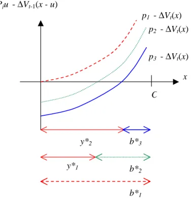
- 14 - Jean Michel Chapuis capacity threshold b*j is reached or the time ends, whichever come first. For an illustration, consider the case where n = 3 and p1 > p2 > p3. and the figure 2.2.
Figure 2-2 : Case with 3 fare classes
2.2.2 The control by time thresholds
Second, consider controlling the revenue through t, the time left, to accept (u = 1) or reject (u = 0) an incoming request. Based on previous properties of equation 1.2., one can show that the optimal policy is characterized by time thresholds. During the booking horizon, they are points in time before which requests are rejected7 and after which requests are accepted8. Since ∆Vt(x) is increasing in t, it follows that pju - ∆Vt-1(x
7 Because one expects to receive booking orders from clients willing to pay high fare (high
opportunity cost), justifying rejection.
8
Because it's too late to expect high fare requests to come (low opportunity cost), in such a quantity to fulfill the capacity.
Pju - ∆Vt-1(x - u) C x y*2 b*3 p3 - ∆Vt(x) p2 - ∆Vt(x) p1 - ∆Vt(x) y*1 b* 2 b*1
- 15 - Jean Michel Chapuis
- u) is decreasing in t. Thus, it is optimal to keep refusing incoming requests (not
increase u in a static formulation) until the previous term becomes positive.
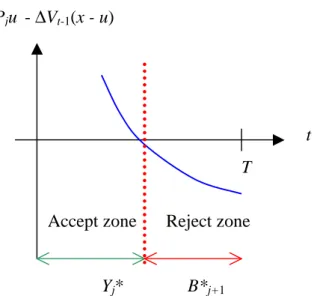
Figure 2-3: critical time threshold
Legend: For a given booking capacity x, a request for a seat of fare class j in decision period t is accepted if time remaining is short (less than Yj*, the critical time threshold) and rejected otherwise. The caps denote that the control is expressed on a time axis instead of a quantity axis.
This proposition is also easy to understand with the figure 2-1. Since ∆Vt(x) is increasing in t, one should accept more booking for a given j when remaining time lessens. In other words, as time elapses, the EMV decreases and the line lifts up. Then the optimal protection level y*j will shift to the left (decrease). The nested protection structure is kind of ...< y*tj−1< y*tj < y*tj+1 <... Pju - ∆Vt-1(x - u) T t Reject zone Accept zone Yj* B*j+1
- 16 - Jean Michel Chapuis
2.2.3 Bid prices
Finally, the optimal control can also be implemented through a table of bid prices, defined as πj+1(x) = ∆Vt(x). A bid price is the minimum amount of money to accept in exchange of a unit of capacity. Under mild assumptions (Gallego and Van Ryzin, 1994; Talluri and Van Ryzin, 1998), the optimal price path πj(x) is decreasing in
x and increasing in t. Dynamic pricing is becoming a real challenge for airlines since
low cost carriers are introducing less restricted fares. For example, Ryanair or Easyjet are not able to be sure that the more price sensitive passengers (low fare) book first. Then they apply a dynamic pricing strategy for a single product without price discrimination between their customers.
3 D
ISCUSSION AND CONCLUSIONThe use of Dynamic Programming in Revenue Management helps to decide whether to accept or reject an incoming booking reservation with more realism than older methods. There are two main points. One proposition of DP in RM is to relax the low-before-high fare order of arrival bookings. In practice, the DP provides the optimal
policy for the RM problem, by evaluating the whole tree of possibilities and making at
each point in time the decision that would imply higher future expected revenues, processing backward recursion. The dark side is the increase in the computation difficulties according to the dimension of the problem. This means that for a single product with 100 units to sell over a 200 time periods, the number of iterations is 100 x 200 = 20 000. But for three products using the same resource, this number becomes 100 x 2003 = 800 millions. Saranathan and Zhao (2005) had related the implementation of DP in United Airlines and that the company expects a 1 to 2 % increase in revenue ($ 158 billions of 2005 turnover).
- 17 - Jean Michel Chapuis The second interest of DP approach, and the main avenue for future research, is that it allows RM to incorporate the consumer choice in the optimization process. El-Haber and El-Taha (2004) formulate a dynamic programming model to solve the seat inventory control problem for a two-leg airline with realistic elements of consumer behavior. Ahead of the Origin and Destination formulation, they consider cancellation, no-shows and overbooking. Following Talluri and Van Ryzin (2003) work, Van Ryzin and Vulcano (2006) consider a revenue management, network capacity control problem in a setting where heterogeneous customers choose among the various products offered by a firm (e.g., different fight times, fare classes and/or routings). Customers may therefore substitute if their preferred products are not offered, even buy up. Their choice model is very general, simply specifying the probability of purchase for each fare product as a function of the set of fare products offered. Overall, the value of our paper is to facilitate the understanding of more complex, and probably more realistic, models of Revenue Management.
4 R
EFERENCESBELLMAN R., 1957, Applied Dynamic Programming, Princeton University Press; BELOBABA P.P., 1989, “Application Of A Probabilistic Decision Model To Airline Seat Inventory Control”, Operations Research, vol. 37, n. 2, pp. 183-198;
BERTSEKAS D., 1995, Dynamic Programming and Optimal Control, Athena Scientific, vol. 1, Belmont MA.;
BERTSIMAS D. AND DE BOER S., 2005, “Dynamic pricing and inventory control for multiple products”, Journal of Revenue and Pricing Management, vol. 3, n. 4, pp. 303-319 ;
BERTSIMAS D AND POPESCU I., 2003, “Revenue Management in a Dynamic Network Environment”, Transportation Science, vol. 37, n. 3, pp. 257-277 ;
BITRAN G. and MONDSCHEIN S., 1995, “An Application of Yield Management to the Hotel Industry considering Multiple Day Stays”, Operations Research, vol. 43, n.3, p. 427–443 ;
- 18 - Jean Michel Chapuis BITRAN G. AND CALDENTEY R., 2003, “An Overview of Pricing Models for Revenue Management”, Manufacturing and Service Operations Management, vol. 5, pp. 202-229;
BRUMELLE, S. AND MCGILL. J.I., 1993, “Airline Seat Allocation with Multiple Nested Fare Classes”, Operations Research, 137;
CHIANG, W-C., CHEN, J.C.H. AND XU, X., 2007, “An Overview of Research on Revenue Management: Current Issues and Future Research”, International Journal of
Revenue Management, vol. 1, n. 1, pp. 97–128.
CURRY R., 1990, “Optimal Seat Allocation with Fare Classes Nested by Origins and Destinations”, Transportation Science, vol. 24, p. 194–204 ;
EL-HABER S. AND EL-TAHA M., 2004, “Dynamic two-leg airline seat inventory control with overbooking, cancellations and no-shows”, Journal of Revenue and Pricing
Management, vol. 3, n. 2, pp. 143-170.
FENG Y. AND GALLEGO G., 2000, « Perishable asset revenue management with Markovian time dependent demand intensities », Management Science, vol. 46, n. 7, p. 941-957 ;
FENG Y. ET XIAO B., 2001, « A dynamic airline seat inventory control model and its optimal policy », Operations Research, vol. 49, n. 6, p. 938-952 ;
GALLEGO G. AND G. VAN RYZIN, 1994. “Optimal Dynamic Pricing of Inventories with Stochastic Demand over Finite Horizons”, Management Science, vol. 40, n.8, pp. 999-1020;
GALLEGO G. AND VAN RYZIN G., 1997, “A Multiproduct Dynamic Pricing Problem and its Applications to Network Yield Management”, Operations Research, vol. 45, n. 1, p. 24-42 ;
KIMES S.E., 1989, “Yield Management: A Tool for Capacity-Constrained Service Firms”, Journal of Operational Management, Vol. 8, n. 4, p.348-64 ;
KLEYWEGT A.J., 2001, “An Optimal Control Problem of Dynamic Pricing”,
Working paper, 25 p. ;
LAUTENBACHER C. AND STIDHAM S., 1999, “The Underlying Markov Decision Process in the Single-Leg Airline Yield Management problem”, Transportation Science, vol. 33, n. 2, p. 136–146 ;
LEE T. AND HERSH M., 1993, “A model for dynamic seat inventory control with multiple seat bookings”, Transportation Science, vol. 27, pp. 233-247 ;
LITTLEWOOD K., 1972, “Forecasting and Control of Passengers Bookings”, Proceeds of AGIFORS, Nathanya, Israel ;
- 19 - Jean Michel Chapuis MCGILL J.I. AND VAN RYZIN G.R., 1999, “Revenue Management: Research Overview and Prospects”, Transportation Science, vol. 33, n.2, pp. 233-257;
PFEIFER P.E., 1989, “The Airline Discount Fare Allocation Problem”, Decision
Sciences, vol. 20, n.1, pp. 149-157;
ROBINSON L.W., 1995, “Optimal and Approximate Control Policies for Airline Booking with Sequential Fare Classes”, Operations Research, vol. 43, n. 1, p. 252-263 ;
SARANATHAN K. AND ZHAO W., 2005, “Revenue Management in the New Management of the New Fare Environment ”, Proceeds of AGIFORS Reservation and Yield Management Study Group, Cape Town;
SMITH B.C., LEIMKUHLER J.F. AND DARROW R.M., 1992, “Yield Management at American Airlines”, interfaces, vol. 22, n. 1, pp. 8-31;
TALLURI K.T. AND VAN RYZIN G.J., 1998, « An aAnalysis of Bid-Price Controls for Network RM », Management Science, vol. 44, n. 11, p. 1577-1594 ;
TALLURI K.T. AND VAN RYZIN G.J., 2003, “Revenue Management under a General Discrete Choice Model of Consumer Behavior”, Management Science, vol. 50, n. 1, p. 15–33 ;
TALLURI K.T. AND VAN RYZIN G.J., 2004, “The Theory and Practice of Revenue Management”, 712 p.;
VAN RYZIN G.J. AND VULCANO G., 2006, “Computing Virtual Nesting Controls for Network Revenue Management Under Customer Choice Behavior”, Columbia
University working paper ;
WOLLMER R., 1992, “An Airline Seat Management Model for a Single Leg Route when Lower Fare Classes Book First”, Operations Research, vol. 40, p. 26-37 ;
YOU P.S., 2001, “Airline Seat Management with rejection-for-possible-upgrade decision”, Transportation science part B, vol. 35, pp. 507-524.
ZHAOW. AND ZHENG Y.-S., 2000, “Optimal Dynamic Pricing for Perishable Assets with Nonhomogeneous Demand”, Management Science, vol. 46, n. 3, p. 375– 388 ;
- 20 - Jean Michel Chapuis
5
APPENDICES5.1 Correspondence between DP and EMSR models
The recommendation about booking acceptance of DP models is similar to the one of EMSR models. For example, suppose there is one seat left to sell, and a potential customer has just called and asked to make a reservation for a discount fare. The flight will take off tomorrow. Thus T = 1, n = 2 (j = 1 – full fare – to 2 – discount fare –), and
{
1}
Pr 1 1
1= D ≥
λ
is the probability of an arrival of class 1 in the period 1 before departure. Since the potential discount customer hold the line, 2 Pr{
2 1}
11 = D ≥ =
λ
. Then equation 1.1. becomes : { }{
(
)
}
+ − = − ∈ p u V x u E x V j t u t 1 1 , 0 max ) ( = { }E p u { }E[
p pu]
{ }{
p p u}
x V u u j j u 2 2 1 1 1 1 1 , 0 2 1 1 , 0 2 1 1 , 0 max max max ) ( = + =λ
+λ
= ∈ ∈ = ∈∑
Then, the manager has to reject while
λ
1p1(1)+ p2(0)is greater thanλ
1p1(0)+ p2(1). In other words, the policy is close fare class j = 1 when1 2 1 p p >
λ
,or when the probability of spoilage is lower than the discount rate offered to customers :
{
}
1 2 1 1 1 Pr p p pD < = − . This is the EMSR rule assuming there is only one seat to sell next period.
- 21 - Jean Michel Chapuis 5.2 Appendix B { }
{
}
{ }{
}
{ }{
[
]
}
{ }{
[ ][
( ) ( )] [
( )]
}
max ) ( ) ( ) ( ] [ max )] ( [ ] [ max ) ( max ) ( 1 1 1 1 , 0 1 1 1 1 , 0 1 1 , 0 1 1 , 0 x V E x V u x V E u p E x V x V u x V E u p E u x V E u p E u x V u p E x V t t t j u t t t j u t j u t j u t − − − ∈ − − − ∈ − ∈ − ∈ + − − + = + − − + = − + = + − =The last term depends neither on the probability of an arrival in period t or the decision u made in t. In other words, this means that the optimization of the revenue from t-1 to 1 depends on neither what have been done before nor what happens today. Moreover, this is the true reason why the model is built assuming the demand is known in t before the decision to make. This term is then equal to Vt-1(x) and can be written out of the E[] and the max functions.
{ }