The impact of model grid zooming on tracer transport in the 1999/2000 Arctic polar vortex

HAL Id: hal-00295353

https://hal.archives-ouvertes.fr/hal-00295353

Submitted on 31 Oct 2003

HAL is a multi-disciplinary open access

archive for the deposit and dissemination of

sci-entific research documents, whether they are

pub-lished or not. The documents may come from

teaching and research institutions in France or

abroad, or from public or private research centers.

L’archive ouverte pluridisciplinaire HAL, est

destinée au dépôt et à la diffusion de documents

scientifiques de niveau recherche, publiés ou non,

émanant des établissements d’enseignement et de

recherche français ou étrangers, des laboratoires

publics ou privés.

in the 1999/2000 Arctic polar vortex

M. M. P. van den Broek, M. K. van Aalst, A. Bregman, M. Krol, J. Lelieveld,

G. C. Toon, S. Garcelon, G. M. Hansford, R. L. Jones, T. D. Gardiner

To cite this version:

M. M. P. van den Broek, M. K. van Aalst, A. Bregman, M. Krol, J. Lelieveld, et al.. The impact of

model grid zooming on tracer transport in the 1999/2000 Arctic polar vortex. Atmospheric Chemistry

and Physics, European Geosciences Union, 2003, 3 (5), pp.1833-1847. �hal-00295353�

Atmos. Chem. Phys., 3, 1833–1847, 2003

www.atmos-chem-phys.org/acp/3/1833/

Atmospheric

Chemistry

and Physics

The impact of model grid zooming on tracer transport in the

1999/2000 Arctic polar vortex

M. M. P. van den Broek1, M. K. van Aalst2, A. Bregman3, M. Krol2, J. Lelieveld4, G. C. Toon5, S. Garcelon6, G. M. Hansford6, R. L. Jones6, and T. D. Gardiner7

1_{Space Research Organization of the Netherlands (SRON), Utrecht, The Netherlands} 2_{Institute for Marine and Atmospheric Research (IMAU), Utrecht, The Netherlands} 3_{Royal Netherlands Meteorological Institute (KNMI), De Bilt, The Netherlands} 4_{Max-Planck-Institut f¨ur Chemie (MPI), Mainz, Germany}

5_{Jet Propulsion Laboratory (JPL), Pasadena, USA} 6_{Cambridge University, Cambridge, UK}

7_{National Physical Laboratory (NPL), Teddington, UK}

Received: 27 January 2003 – Published in Atmos. Chem. Phys. Discuss.: 9 May 2003 Revised: 8 October 2003 – Accepted: 17 October 2003 – Published: 31 October 2003

Abstract. We have used a 3-D chemistry transport model to evaluate the transport of HF and CH4in the stratosphere

during the Arctic winter of 1999/2000. Several model ex-periments were carried out with the use of a zoom algorithm to investigate the effect of different horizontal resolutions. Balloon-borne and satellite-borne observations of HF and CH4 were used to test the model. In addition, air mass

de-scent rates within the polar vortex were calculated and com-pared to observations.

Outside the vortex the model results agree well with the observations, but inside the vortex the model underestimates the observed vertical gradient in HF and CH4, even when

the highest available resolution (1◦×1◦) is applied. The cal-culated diabatic descent rates agree with observations above potential temperature levels of 450 K. These model results suggest that too strong mixing through the vortex edge could be a plausible cause for the model discrepancies, associated with the calculated mass fluxes, although other reasons are also discussed.

Based on our model experiments we conclude that a global 6◦×9◦resolution is too coarse to represent the polar vortex, whereas the higher resolutions, 3◦×2◦and 1◦×1◦, yield sim-ilar results, even with a 6◦×9◦resolution in the tropical re-gion.

Correspondence to: M. M. P. van den Broek

(broekvd@knmi.nl)

1 Introduction

Both 2-D and 3-D Chemistry Transport Models (CTMs) are widely used to evaluate the understanding of atmospheric processes and to study how possible future changes in emis-sions will affect the composition and state of the atmosphere. One important focus of stratospheric research with CTMs is the depletion of ozone, notably in the polar vortex and at mid-latitudes. Both transport and chemical processes influ-ence the ozone concentration, while its variability is mainly determined by dynamics (Chipperfield and Jones, 1999). To model stratospheric ozone and to estimate chemical ozone loss, it is therefore of great importance that ozone transport is modeled realistically.

Several studies tested modeled transport and investigated the related key model properties. In a 2-D latitude-longitude study on ozone depletion, Edouard et al. (1996) found a large impact of increasing horizontal resolution. Searle et al. (1998) repeated this study with contradictory results. Since both these studies concentrate on ozone depletion, both chemistry and transport are expected to influence this result. One method to evaluate model transport separately is by simulating long-lived tracers, which can then be tested against observations. HF, for example, is such a tracer, which is used in this study. In an earlier model evaluation, Chip-perfield et al. (1997) also simulated HF. They found a good agreement with observations, except in polar air where HF columns were underestimated. Rind et al. (1999) used CFC-11 and SF6 to evaluate model transport across the tropopause and found no improvement when they increased the vertical resolution of their general circulation model (GCM). They suggested that dynamical properties such as wave drag and

1834_{shown here.} M. M. P. van den Broek et al.: The impact of model grid zooming on tracer transport

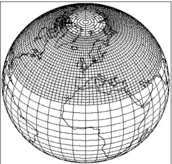
Fig. 1. An illustration of the horizontal zoom grid of TM5. Zoom

option Gl96 NH32 is shown here.

top altitude of the model should be improved with priority. Mahowald et al. (2002) point out that the choice of the ver-tical coordinate system, based on pressure or isentropes, im-pacts tracers such as water vapor and the age of air in the tropical stratosphere, with the isentropic coordinate system giving less diffusive and more realistic model results. A recent model intercomparison among 2-D models and 3-D CTMs showed that the calculated age of air was too low in almost all models (Hall et al., 1999). However, more recent analysis showed that the descent rates inside the polar vortex in the 3-D CTMs SLIMCAT and REPROBUS agreed reason-ably well with observations (Greenblatt et al., 2002). Plumb et al. (2002) modeled transport of N2O in the polar vortex for

the same winter using the CTM MATCH. They found that N2O was overestimated in the lower stratospheric vortex and

suggested that cross-vortex boundary transport was not accu-rately calculated or that inner-vortex mixing was too intense. It was suggested that this was related to the underlying mete-orological data, since doubling their original horizontal reso-lution of 2.8◦×2.8◦did not make a difference. Another study of N2O and NOy transport during this winter showed that

in-creasing the vertical resolution did not improve the compar-ison of model results with observations either (Considine et al., 2003).

In this study we explore the effect of horizontal resolu-tion and of using a zoom region on tracer distriburesolu-tions in more detail by model simulations of HF and CH4during the

1999/2000 winter, focusing on the Arctic polar vortex. We also evaluate diabatic descent rates to interpret the calculated tracer distributions. We employ the newly developed chem-istry transport model TM5 (Krol et al., 2003) to simulate

HF and CH4. TM5 contains a 2-way nesting zooming

al-gorithm (Krol et al., 2001), which is employed here to study the effect of resolution changes on transport. HF and CH4

are long-lived in the stratosphere and have lifetimes over 1 year below 10 hPa, and are therefore solely influenced by transport on shorter timescales. HF is produced in the up-per stratosphere by photochemical breakdown of CFCs. It has no chemical sinks in the stratosphere and its only known loss mechanism is downward transport and subsequent wet deposition in the troposphere. CH4 has the inverse profile,

with higher values in the troposphere due to emissions at the earth surface from biogenic and anthropogenic activity. Con-centrations drop with increasing altitude due to chemical loss by photo-dissociation and reaction with OH, O1D and Cl in the stratosphere and reaction with OH in the troposphere.

An important reason to focus on the 1999/2000 winter is the availability of observations of HF and CH4from the

com-bined SOLVE (Sage III Ozone Loss and Validation Experi-ment) and THESEO (THird European Stratospheric Exper-iment on Ozone) campaigns. Furthermore, a distinct polar vortex formed in the lower stratosphere after December 1st (Manney and Sabutis, 2000), which provides a good test case to study the isolation of the vortex.

We investigate modeled tracer distributions employing three different horizontal resolutions in the northern hemi-sphere, ranging from 9◦ longitude by 6◦ latitude to 1◦ lon-gitude by 1◦latitude. Van Aalst et al. (2003) carried out a model study with the same experimental set-up, using the MA-ECHAM climate model with assimilated meteorologi-cal data of the same time period.

The model experiments and the observations used are de-scribed in Sect. 2. Section 3 presents the model results and compares with the observations. A sensitivity test on the model initialization is carried out in Sect. 3.6. Discussion and conclusions follow in Sect. 4.

2 Model experiments 2.1 Model description

We have used the new global three-dimensional transport model, version 5 (TM5). The model is an extended ver-sion of the TM3 model that has been used in several previous stratospheric studies (Van den Broek et al., 2000; Bregman et al., 2000; Bregman et al., 2001). The new model is able to zoom horizontally over a certain area, e.g. Europe or the po-lar vortex, by selectively increasing the horizontal resolution. Krol et al. (2001) explain the mass conserving two-way nest-ing algorithm and show first model results for tropospheric

222_{Rn. Figure 1 gives an impression of the zooming}

op-tions in TM5 used in this study. Meteorological input for the model is provided by six-hourly ECMWF (European Cen-tre for Medium-Range Weather Forecasts) forecast fields of temperature, surface pressure, wind and humidity. The data

M. M. P. van den Broek et al.: The impact of model grid zooming on tracer transport 1835

Table 1. An overview of the different horizontal resolutions used in

this study

Region 1 (global) lon×lat Region 2 (zoom) lon×lat Gl 96 9◦×6◦

Gl96 NH32 9◦×6◦ 3◦×2◦(24◦N–90◦N) Gl 32 3◦×2◦

Gl32 NP11 3◦×2◦ 1◦×1◦(30◦N–90◦N)

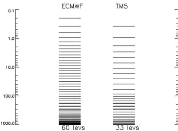
extend up to 0.2 hPa. The method to calculate mass fluxes from ECMWF winds has recently been improved (Bregman et al., 2003). We used a 33-layer subset of the 60 layer fields that are taken into account in the ECMWF model, with a re-duced number of levels in the tropospheric boundary layer and above 70 hPa. Before 12 October 1999 the ECMWF model used 50 vertical layers from which we derived a subset of 30 layers. Near the surface the model levels are defined as terrain following sigma coordinates whereas the layers above 100 hPa are defined at pressure surfaces. A hybrid of the two is used between the lower levels and the lower stratosphere. An example of the vertical grid in TM5, assuming a surface pressure of 1000 hPa, is shown in Fig. 2 together with the original ECMWF grid.

A mass flux advection scheme, using first order slopes (Russell and Lerner, 1981), is used to calculate tracer trans-port. A dynamical time step of 1800 s is applied for the coars-est grid (6◦latitude by 9◦longitude). For the 1◦by 1◦ resolu-tion a time step of 225 s is employed. Over the poles, the grid is reduced to avoid numerical instability through violation of the Courant Friedrichs-Lewy (CFL) condition (see Fig. 1). The physical parameterization of boundary layer diffusion and convection are identical to those of the TM3 model (Pe-ters et al., 2002), For instance, convection is calculated with the Tiedtke (1989) mass flux parameterization for cumulus clouds, including entrainment and detrainment in updrafts and downdrafts.

2.2 Experimental set-up

In this study, HF, and CH4are simulated for the Arctic

win-ter of 1999–2000. Four zooming options have been investi-gated (see Table 1), with a horizontal model resolution rang-ing from 9◦longitude by 6◦latitude globally, up to 1◦by 1◦ from 30◦to 90◦N.

The model integrations start at 1 September 1999. Ini-tialization is based on zonally averaged observations of the HALOE (HALogen Occultation Experiment) sunset sweep of 7 August to 22 September 1999, which ranged from 73.9◦N to 63.5◦S. In regions for which observations are not available (at the poles, in the troposphere and in a gap in the HALOE data between 43◦N and 62◦N), the ini-tial concentrations are linearly inter- or extrapolated from nearby latitudes. In the vertical direction, we prescribe

tropo-Figure 2.The vertical grid of TM5 and the original ECMWF vertical grid.

Fig. 2. The vertical grid of TM5 and the original ECMWF vertical

grid.

spheric values of 0 ppbv HF and 1.76 ppmv CH4, distributed

slightly over the two hemispheres by adding a 0.02 ppmv sine function. A log-pressure interpolation is applied when no HALOE data are available at a certain altitude.

Removal of HF by wet deposition has been implemented in TM5 by assuming a lifetime of 5 days below 400 hPa, as in Chipperfield et al. (1997). In the top two levels CH4and HF

are constrained with monthly zonally averaged UARS data (Randel et al., 1998), since chemical production (of HF) and destruction (of CH4) are not included in the model.

Sensi-tivity runs carried out by Van Aalst et al. (2003) show that stratospheric washout of HF and prescribing the top bound-ary concentrations for both tracers have only a small or neg-ligible effect on the tracer fields for the integration period considered in this study. In addition, they found that ignor-ing chemical destruction of CH4causes a small deviation of

less than 10%, and only above 20 hPa.

2.3 Observations during the 1999–2000 winter

The lower stratosphere was extremely cold during the Arctic winter of 1999–2000, especially in the early winter. Despite these low temperatures, the lower stratospheric vortex was weak until December and formed slowly compared to other cold winters. In the upper and middle stratosphere, a dis-tinct vortex was already discernable on 1 November. By the end of December, the vortex was established throughout the stratosphere (Manney and Sabutis, 2000).

Several measurements of CH4and HF were used for

com-parison with the model results. (i) The balloon-borne Tun-able Diode Laser Absorption Spectrometer (TDLAS) mea-sured in-situ profiles of CH4. The flights took place on 28

January, 9, 13, and 27 February and 25 March 2000 and samples were taken inside, outside and at the edge of the vortex (Garcelon et al., 2002). (ii) Balloon-borne observa-tions of HF and CH4 were carried out with the JPL MkIV

0 .5 1. 1.5 _{0 .5} 1. 1.5 0 .5 1. 1.5 2. 2. 1. 1.5 .5

R-0.921

No.=694

R=0.957

No.=694

R=0.962

No.=694

Gl96 run

Gl32 run

Gl32_NP11 run

HALOE HF [ppbv]

TM

5

H

F

[p

pb

v]

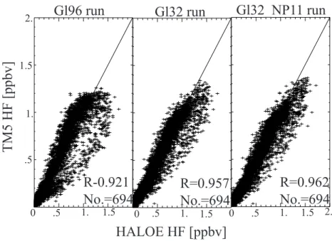
Fig. 3a. Correlation between HALOE observations and TM5 model output for three different model resolutions: Gl96 (9◦×6◦), Gl32 (3◦×2◦) and Gl32 NP11 (1◦×1◦, 3◦×2◦south of 30◦N), from December 1999 to March 2000, north of 30◦N and pressure <150 hPa. The number of profiles used is given as well.

interferometer (Toon et al., 1999) in the inner vortex; both at the start of vortex formation on 3 December 1999 and close to vortex break up on 15 March 2000. (iii) The HALOE in-strument observed both CH4and HF, collecting 8–15 profiles

each day at two latitude bands (Russell et al., 1993). Usually, HALOE observations do not extend poleward far enough to reach the vortex, but on 20 February 2000 at 56◦N some pro-files were obtained at the edge of the vortex.

All these observations have been compared with the TM5 results. In addition, diabatic descent rates within the vortex, calculated by the model, have been compared with those de-rived from CH4observations (Greenblatt et al., 2002).

3 Results

3.1 HALOE HF profiles

The HALOE instrument has sampled many mid-latitude pro-files of HF during the ’99-’00 winter. The errors within the HALOE HF profiles are small. The mean difference be-tween HALOE HF and correlative balloon underflight mea-surements is less than 7% in the altitude range between 5 hPa and 50 hPa (Russell et al., 1996).

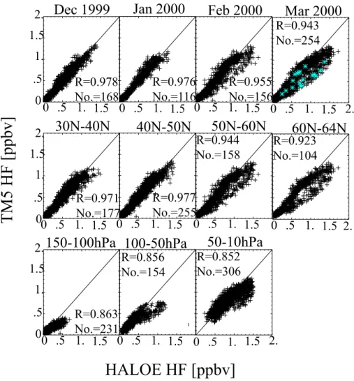
All available Northern hemispheric mid-latitude HALOE HF observations from December 1999 to March 2000 have been compared to the modeled fields. North of 30◦N, 649 profiles were measured in total. The bulk of the measure-ments were carried out outside the polar vortex. Figures 3a and b show the correlations of these observations with the TM5 model results. The TM5 results have been matched

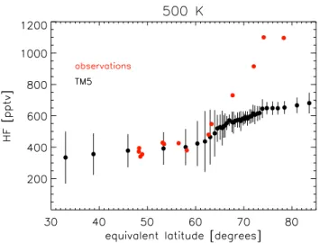
with the measurements by using the results of the model grid-box and time zone (within 12 hours) in which the HALOE data were observed. Since the HALOE instrument pro-duces a high vertical resolution compared to the TM5 model, HALOE observations within one TM5 vertical layer have been averaged. Figure 3a shows all correlations for 3 dif-ferent horizontal model resolutions: 9◦×6◦ (Gl96), 3◦×2◦ (Gl32) and 1◦×1◦(Gl32 NP11, with 3◦×2◦south of 30◦N). Independent of resolution, the correlation between the model results and the observations is good. The gl69 run shows the largest scatter with a tendency to underestimate the tracer distribution. The results from higher resolutions show much less scatter. Note that the correlation hardly improves any further when going from a 3◦_×2◦ _{to a 1}◦_×1◦ _resolution. Nevertheless, significant variability is present, even at the highest resolution. We have separated these relationships in time, latitude, and pressure to investigate the origin of this variability. Figure 3b shows the results from the gl23 run. The significant underestimation becomes primarily visible at the end of the winter (March) at high latitudes between 50– 100 hPa. We have selected 15 March 2000 to show that the samples of this “branch” of data originate from the polar vor-tex (blue crosses). We therefore compared the model results with all HALOE profiles on 15 March on an equivalent lati-tude grid at a potential temperature level of 500 K in Fig. 3c. One can clearly see that the model deviates at high equivalent latitudes. The agreement is good at midlatitudes where all observations fall within the model variability (2σ ) for each equivalent latitude bin. This indicates that the model devia-tions only occur in polar vortex air.

M. M. P. van den Broek et al.: The impact of model grid zooming on tracer transport 1837

0 .5 1. 1.5 0 .5 1. 1.5 0 .5 1. 1.5 0 .5 1. 1.5

0 .5 1. 1.5 0 .5 1. 1.5 0 .5 1. 1.5 0 .5 1. 1.5

0 .5 1. 1.5

0 .5 1. 1.5

0 .5 1. 1.5

2.

2.

2.

2.

1.

1.5

.5

0

2.

1.

1.5

.5

0

2.

1.

1.5

.5

0

Dec 1999

Jan 2000

Feb 2000

Mar 2000

30N-40N

40N-50N

50N-60N

_60N-64N

150-100hPa 100-50hPa

50-10hPa

HALOE HF [ppbv]

TM

5

H

F

[p

pb

v]

R=0.978

No.=168

R=0.976

No.=116

R=0.955

No.=156

R=0.943

No.=254

R=0.971

No.=177

R=0.977

No.=255

R=0.944

No.=158

R=0.923

No.=104

R=0.863

No.=231

R=0.856

No.=154

R=0.852

No.=306

Fig. 3b. Correlation between HALOE observations and TM5 model output for the Gl32 run, divided among 4 time periods (December

1999–March 2000), 4 latitudes (30–40◦N, 40–50◦N, 50–60◦N and 60–63◦N) and 4 altitude regions (150–100 hPa, 100–50 hPa, 50–10 hPa, 10–1 hPa). For the different time periods and latitudes, the number of profiles is given as well (15 comparisons per profile). The blue crosses denote observations of 15 March between 100 and 50 hPa.

3.2 TDLAS CH4observations in/out of the vortex

As a next step, we compared modeled CH4profiles to CH4

profiles that have been measured by means of the balloon-borne TDLAS spectrometer, both inside and outside the po-lar vortex. The result is shown in Fig. 4a. The estimated er-ror for the observations is about 10% (Garcelon et al., 2002). Clearly, as in Fig. 3, the model results compare reasonably well with the observations outside the vortex, whereas the model results within and at the inner edge of the vortex indi-cate significant overestimation. As in Fig. 3, it is remarkable that the model results are very similar for all zooming ex-periments, including the 1◦by 1◦resolution. The Gl 96 run shows the largest overestimation, implying that this resolu-tion is too coarse for a realistic representaresolu-tion of the tracer distribution.

The good agreement between model and observations out-side the vortex was also indicated by the HALOE profile

comparisons, especially below 10 hPa (see Fig. 3). However, inside and at the edge of the vortex the CH4vertical gradient

increases with time, which is obviously not fully captured by the model.

Figure 4b shows the modeled horizontal gradients on a pressure level of approximately 75 hPa across the vortex edge between Kiruna, the site of the balloon observation, and cen-tral Europe on 13 February 2000. The coarser Gl 96 model run results in a gradient of ∼0.1 ppmv between Kiruna and central Europe, whereas the Gl 32 and NP 11 runs gives a larger gradient of ∼0.2 ppmv. Nevertheless, these gradients are smaller than the differences between the model and the observation at this altitude, which is about 0.35 ppmv (see Fig. 4a). The 1◦by 1◦run does show a sharper gradient, as can be expected, with more distinct features. This may be important when species with large concentration gradients over the vortex edge are studied.

Fig. 3c. HF volume mixing ratio from HALOE observations

(aster-isks) and TM5 simulations (black dots), along equivalent latitude. Results are shown for 15 March 2000 on the 500 K potential tem-perature level. The vertical bars denote the model variability (2σ ) for each equivalent latitude bin (2◦).

3.3 MkIV inner vortex observations in early and late winter In Fig. 5 TM5 results are compared to HF and CH4

mea-surements by the MkIV interferometer, focusing here on the lower stratosphere. The observations were carried out inside the polar vortex in the beginning of winter, on 3 December, when the vortex was just formed in the lower stratosphere, and on 15 March 2000, just before the vortex break-up. Also in this comparison, HF is consistently underestimated and CH4is overestimated, both at the beginning and at the end of

winter, and the differences between the model runs are simi-lar to the earlier comparisons. However, on 3 December, the difference between model and observation occurs only above 50 hPa while by March 15, the difference is seen throughout the lower stratosphere. Above 15 hPa HF steeply decreases and CH4increases on 15 March. PV maps indicate that the

MkIV observations above 15 hPa were at the edge of, or out-side, the vortex, which explains the gradient reversal. The discrepancies found so early in winter suggest a potential im-pact from inaccuracies in the initial tracer field. Later we will demonstrate the sensitivity of the model results for the initial tracer fields.

3.4 HALOE HF longitude cross section

Fifteen HALOE HF sunrise profiles, observed on 20 Febru-ary 2002 at 56◦N, have been compiled in a longitudinal graph and are compared with TM5 results (Fig. 6). The HALOE observations comprise both vortex and non-vortex air. For example, the feature with increased HF values be-tween 90◦E and 60◦E and 50 Pa and 10 hPa represents air from the vortex edge. An increased vertical gradient in HF is visible below this area, between 100 hPa and 20 hPa. Another

small feature of increased HF is discernable near 100 hPa, around 150◦_E–180◦_E.

More obvious than in the previously discussed profile comparisons, the Gl 96 run is too coarse to simulate trans-port within or across the edge of the vortex, since none of the observed longitudinal features is captured (Fig. 6b). All other model runs capture the observed longitudinal features well and again they produce similar results. On the other hand, the model underestimates the vertical gradient between 100 hPa and 1 hPa at all longitudes, and especially inside the vortex between 150◦E and 180◦E. This is in agreement with the profile comparisons discussed above (Figs. 4 and 5). The discrepancy between 10 and 1 hPa is also visible in the late winter mid-latitude profiles shown in Fig. 3 and may be at-tributed to the mixing of vortex air with mid-latitude air.

The vortex air sampled at 56◦N was situated at the edge, which can be seen from the modeled latitudinal cross-sections at 50◦N and 62◦N (not shown here). The represen-tation of the vortex edge may contribute to the discrepancies with the observations there, due to the large gradients of HF across the edge of the vortex. At 62◦N for example, situated more inside the vortex, the sharp vertical gradient matches much better with the HALOE observations at 56◦_{N (see also} van Aalst et al., 2003).

3.5 Descent rates

One likely cause of the model-observations discrepancies could be the underestimate of the diabatic descent by the model. To evaluate the possible origin of these discrepan-cies, we calculated the modeled vertical descent rates inside the vortex from 1 December to 1 March 2000 and compared those with observed descent rates (i.e. derived from observa-tions). It should be kept in mind that such comparisons do not separate vertical and horizontal transport, so that devia-tions can be caused by inaccuracies in the mass flux repre-sentation in TM5 in both directions. The observed descent is derived from a number of CH4observations inside the vortex

and agrees with calculations carried out with a large number of N2O observations (Greenblatt et al., 2002).

Figure 7 shows the decrease of potential temperature along five CH4 isopleths throughout the winter. The black

lines shows inner vortex descent calculated from five ob-served profiles of CH4 during the SOLVE/THESEO

cam-paign [Greenblatt et al., 2002]. The red lines represent the descent of CH4calculated with TM5. On each first day of

the month, zonal winds and PV gradients were used to calcu-late vortex average profiles of potential temperature and CH4

(see also van Aalst et al. [2003]). We restricted the sampling to those profiles that were located within the vortex in the full altitude range between 100 and 10 hPa. Inner vortex air was selected by sampling within the area bordered by the steepest gradient in PV, according to the ECMWF forecasts.

Figure 7 shows that, except for the “Gl 96” run, the cal-culated descent rates during the winter agree quite well with

M. M. P. van den Broek et al.: The impact of model grid zooming on tracer transport 1839 TDLAS obs. Gl96 Gl96_NH32 Gl32 Gl32_NP11 10 100 1000 P [h Pa ] 10 100 1000 P [h Pa ] 10 100 1000 P [h Pa ] 10 100 1000 P [h Pa ] 10 100 1000 P [h Pa ] 0.0 0.5 1.0 1.5 2.0 CH4 [ppmv] 0.0 0.5 1.0 1.5 2.0 CH4 [ppmv] 0.0 0.5 CH4 [ppmv]1.0 1.5 2.0 0.0 0.5 1.0 1.5 2.0 CH4 [ppmv] 0.0 0.5CH4 [ppmv]1.0 1.5 2.0

Jan 28 2000 (in vortex)

_{Feb 09 2000 (out)}

Feb 13 2000 (edge)

Feb 09 2000 (edge)

Mar 25 2000 (out)

Fig. 4a. Modeled CH4[ppmv] compared to TDLAS profiles, on 28 January, 9, 13 and 27 February and 25 March 2000.

those observed, except in the layer below θ ∼450 K, which is the layer undergoing the highest ozone loss. The discrepancy increases closer to the vortex lower boundary, i.e. ∼400 K, especially in early winter. Largest descent takes places from December to January, slowing down in February and being

close to zero after the first of March. Increasing the hori-zontal resolution in the zooming experiments, either in the tropics or in the polar region, has no effect on these results.

Initially, modeled potential temperature on 1 December 1999 has been synchronized with the observed θ profiles.

1.61 1.59 1.57 1.55 1.53 1.51 1.49 1.47 1.45 1.43 1.41 1.39 1.37 1.35 1.33 1.31 1.29

80N

50N

10E

30E

NP11, CH4 [ppmv] Feb 13 2000 ~`75hPa

*

80N

Gl32, CH4 [ppmv] Feb 13 2000 ~`75hPa

50N

10E

30E

10E

30E

Gl96, CH4 [ppmv] Feb 13 2000 ~`75hPa

80N

50N

Fig. 4b. Horizontal field of CH4

[ppmv] around Kiruna on 13 Febru-ary 2000, at a pressure level of ap-proximately 75 hPa. The three dif-ferent model runs, NP 11, Gl 32 and Gl 96 show how horizontal gradients across the vortex edge are affected by the model resolution.

M. M. P. van den Broek et al.: The impact of model grid zooming on tracer transport 1841

HF, Dec 3 1999

HF, Mar 15 2000

CH4, Dec 3 1999

CH4, Mar 15 2000

10

100

P

[h

Pa

]

10

100

P

[h

Pa

]

10

100

P

[h

Pa

]

10

100

P

[h

Pa

]

0

0.5

1.0 1.5

2.0

0

0.5

1.0 1.5

2.0

0

_0.5

1.0 1.5

2.0

0

_0.5

1.0 1.5

2.0

[ppbv]

[ppbv]

[ppbv]

[ppbv]

Fig. 5. Modeled HF [ppbv] and CH₄[ppmv] compared to MkIV profiles on 3 December 1999 and 15 March 2000.

Note that at the start of this calculation on 1 December, the offset in potential temperature for comparable CH4 volume

mixing ratios is about 50 K above 500 K. Around 450 K the offset is 20 K, whereas the offset has disappeared around 400 K and layers below. Thus, the model does not simu-late the tracer fields above 450 K correctly, at the start of this comparison on 1 December. This is in agreement with the modeled overestimation of CH4and underestimation of HF

with respect to the MkIV observations on 3 December, illus-trated in Fig. 5.

Similar pre-winter offsets are also found with the 3-D CTMs REPROBUS and SLIMCAT using the same set of ob-servations (Greenblatt et al., 2002). Greenblatt et al. (2002) compared modeled and observed descent rates in a similar

way as discussed here. Both models showed similar descent rates as TM5, although REPROBUS descent is somewhat faster than the observed descent in the beginning of winter in the lower stratosphere. In addition, similar results are found with the MA-ECHAM model (van Aalst et al., 2003). 3.6 Sensitivity of the initialization

The model validation gives arguments to question the influ-ence of the initial fields on the tracer distribution, as men-tioned earlier. The initialization of the model on 1 Septem-ber 1999 was based on the HALOE observations of August and September 1999. The northernmost latitude in this field is 73.9◦N. Therefore the species concentrations in the polar region outside the observed area were extrapolated from this

V e rs ion_ 1 9 /3 0 8 4 _ 3 0 8 4 . gif 1.80 1.62 1.44 1.26 1.08 0.90 0.72 0.54 0.36 0.18 0.0 0 60 120 180 -120 -60 0 0.01 0.10 1.00 10.0 100. longitude P [h Pa ] b. HF, Feb 20 2000, Gl96 d. HF, Feb 20 2000, Gl23 c. HF, Feb 20 2000, Gl96_NH32 0.2 1.0 10. 100 P [h Pa ] 0.2 1.0 10. 100 P [h Pa ] 0.2 1.0 10. 100 P [h Pa ] 180 0 60 120 -120 -60 0 longitude 180 0 60 120 -120 -60 0 longitude 180 0 60 120 -120 -60 0 longitude e. HF, Feb 20 2000, Gl23_NP11 180 0 60 120 -120 -60 0.2 1.0 10. 100 0 longitude P [h Pa ]

a. HALOE HF Press. vs Longit. Sunrise Feb 20 2000 at 56 N

Fig. 6. Modeled HF [ppbv] compared to HALOE observations on 00-02-20, longitudinal cross section at 56◦N.

latitude. Despite this caveat, the method was applied to use as much observations as possible. Another option for initial-ization is the use of 3-D model output fields of full chemistry runs.

To test the impact of the initial fields we have performed a run with the Gl32 resolution, starting on 20 October 1999 and using an initialization provided by the full chemistry ARPROBUS climate model (WMO, 1999). A CTM model study using the same initialization and meteorological input showed a good agreement with inner vortex CH4profiles (G.

Barthet and F. Lef`evre, personal communication).

Figure 8 shows a comparison with the TDLAS and MkIV balloon observations similar to Figs. 4a and 5, with the old and new initialization. The new initialization has resulted in consequently lower CH4 concentrations. Inside the vortex,

this means that the model gives more realistic results. The deviation with the two TDLAS profiles sampled outside the vortex is small as well, in both model runs.

Figure 9 shows the dependence of the correlation between HALOE observations and TM5 results on the initialization. All data from December 1999– March 2000, north of 30?N have been included. As mentioned earlier, the bulk of these

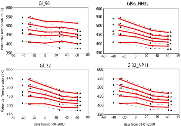
M. M. P. van den Broek et al.: The impact of model grid zooming on tracer transport 1843 600 550 500 450 400 350 600 550 500 450 400 350 600 550 500 450 400 350 600 550 500 450 400 350

Gl_96

Gl96_NH32

Gl32_NP11

Gl_32

Fig. 7. Potential temperature throughout the winter of 1999–2000 along CH4isopleths for observations (Greenblatt et al., 2002) in

black-dotted lines, with the triangles representing the profile observations, and for model results on each first day of the month (red circles connected by solid lines) from all zooming options.

observations are outside the polar vortex. From these re-sults it can be seen that the original HALOE initialization gives a slightly better correlation with the observations. The ARPROBUS initialization gives lower model concentrations. In agreement with the HF comparisons (Figs. 3a, b and c), the samples showing overestimation all originate from the polar vortex. The shift caused by the ARPROBUS initialisation results in better agreement for polar vortex air and slightly worse agreement for extra-vortex air, although the correla-tion remains good. Thus, this figure clearly shows that the initialization does have an effect on the results. However, it does not affect the relative difference between mid-latitudes and the polar vortex.

4 Discussion and conclusions

We have evaluated the 3D chemistry transport model TM5 with the stratospheric tracers HF and CH4during the Arctic

winter of 1999/2000 and tested the new model zooming algo-rithm. The results of our model experiments, applying three different resolutions of 6◦×9◦, 3◦×2◦and 1◦×1◦, have been compared to observations. As can be expected, the coars-est resolution of 6◦latitude by 9◦ longitude produces rela-tively large errors. The longitudinal variation as compared to the HALOE HF observations near the vortex edge, and

inner vortex descent are simulated unrealistically with this resolution. Such discrepancies should be considered since many climate model integrations are performed with similar resolutions (e.g. Pawson et al., 2000, Austin et al., 2003). Outside the vortex, the results of the 2◦_{by 3}◦_{run agree} bet-ter with the observations. Remarkably, the tracer profiles are similar if a 6◦by 9◦resolution is used in the southern hemi-sphere and tropics instead of 2◦by 3◦. Apart from the sig-nificant improvement when increasing the resolution from 9◦ by 6◦to 3◦by 2◦, further increase of the horizontal resolu-tion does not improve, or worsen, the comparison with the observations in this model set-up. Nevertheless, differences between the 3◦×2◦and the 1◦×1◦runs arise close to large gradients such as the vortex edge, which may be important when species with larger concentration gradients are studied. The close resemblance between the results of the uniform 3◦_×2◦ _{run and the northern hemisphere 3}◦_×2◦ _{run shows} the applicability of the TM5 zooming algorithm. Thus, high-resolution simulations become feasible. It is intended to compare these simulations to observations from measure-ments campaigns and satellite instrumeasure-ments in the (lower) stratosphere.

The model comparisons with balloon and satellite profiles measured inside the vortex give an underestimation of HF and subsequent overestimation of CH4for each resolution.

balloon obs. Init. ARPROB. Init. HALOE 10 100 1000 P[ hP a] 10 100 1000 P[ hP a] 10 100 1000 P[ hP a] 10 100 1000 P[ hP a] 10 100 1000 P[ hP a] 10 100 1000 P[ hP a] 10 100 1000 P[ hP a] 0. 0.5 1.0 1.5 CH4 [ppmv] 2.0 0. 0.5CH4 [ppmv]1.0 1.5 2.0 0. 0.5_{CH4 [ppmv]}1.0 1.5 2.0 0. 0.5_{CH4 [ppmv]}1.0 1.5 2.0 0. 0.5_{CH4 [ppmv]}1.0 1.5 2.0 0. 0.5 1.0 1.5 CH4 [ppmv] 2.0 0. 0.5CH4 [ppmv]1.0 1.5 2.0

TDLAS 2000-01-28 (in vortex)

TDLAS 2000-02-09 (out)

TDLAS 2000-02-13 (edge)

TDLAS 2000-02-27 (edge)

TDLAS 2000-03-25 (out)

MkIV 1999-12-03 (in)

MkIV 2000-03-15 (in)

Fig. 8. TDLAS and MkIV balloon-borne observations of CH4from 3 December to 25 March 2000 compared to TM5 output with two

different initialisations. The TDLAS measurements are both inside and outside the vortex, whereas the MkIV measurements are all sampled inside the vortex.

M. M. P. van den Broek et al.: The impact of model grid zooming on tracer transport 1845

R=0.906

R=0.889

HALOE CH4 [ppmv]

TM

5

C

H

4

[p

pm

v]

Init. ARPROBUS

Init. HALOE

Fig. 9. Correlation between HALOE observations and TM5 model output from December 1999 to March 2000, for two different

initializa-tions. These are described in detail in the text.

Our model analysis shows that these model deviations are restricted to polar vortex air. Outside, the HF and CH4

dis-tribution are simulated in agreement with observations. Comparisons with observed tracer isopleths show reason-able agreement in vortex descent for the higher grid reso-lutions. However, this comparison does not separate hori-zontal and vertical model transport, so that both may have contributed to the discrepancies. A way to separate hor-izontal and vertical transport was described by Considine et al. (2003). They isolated the vertical model transport by eliminating tracer concentration gradients along the isen-tropic model levels. Their conclusions point towards com-pensating errors in the vertical and the horizontal transport.

Additional aspects of the exerimental set-up may have contributed to the inner vortex discrepancy. Firstly, it can be ruled out that these discrepancies are caused by uncertainties in boundary conditions at the top and bottom of the model and tropospheric rain-out, as was investigated by van Aalst et al. (2003).

Secondly, some of the comparisons between model and measurements in early winter suggest that the initialization could be in error. The combined time series of the calcu-lated and observed CH4 and HF profiles (Figs. 4a and 5)

show that the inner vortex discrepancy already starts during early winter (note that the discrepancy is already present on 3 December). We tested whether a different initialization was able to explain the discrepancies. A better agreement with observations was indeed achieved within the vortex region,

explaining the early winter offset. It, however, leads to a worse agreement at mid-latitudes (Fig. 9). Thus, an inaccu-rate initialization may lead to an offset, but it cannot fully explain the discrepancies found in the vertical gradient and over time.

Another possible reason for the model discrepancies could be found in the vortex formation. The ECWMF data extend only to 0.2 hPa where observations become sparse. Since the vortex was already formed on 1 November in the upper stratosphere (Manney and Sabutis, 2000), this region is very critical when simulating the early winter vortex. It may indi-cate that either diabatic descent or horizontal transport is not well represented in the model, thus the underlying meteo-rology from ECMWF does not properly represent the down-ward or horizontal transport in the polar vortex. In this study, we increased the horizontal resolution of TM5 up to 1◦×1◦ for a relatively large area (northward of 30◦N). Nevertheless, the discrepancies remain, which may be an indication that the accuracy of the mass fluxes as provided by ECMWF is insuf-ficient (Considine et al., 2003; Plumb et al., 2002). Recent studies indicate that errors in the stratospheric circulation in assimilated meteo fields exist that may play a crucial role here, e.g. during the formation of the winter vortex (Kawa et al., 2003).

Finally, other model characteristics such as the vertical resolution, the advection scheme and the reduced grid used in the polar region have not been investigated. All of these parameters are being addressed with the TM5 model by

including all (60) ECMWF model layers, by removal of the reduced grid and by using a higher order advection scheme (Krol et al., manuscript in preparation).

Acknowledgements. The authors wish to express their gratitude to

the HALOE team for providing us with their observations. We thank the other members of the TDLAS and MkIV teams, especially I. H. Howieson, N. R. Swann and P. T. Woods from the National Physical Laboratory. Benedikt Steil, Christoph Br¨uhl from the Max Planck Institute for Chemistry in Mainz and J. Greenblatt, at Prince-ton University, are thanked for fruitful discussions. The second ini-tialization was provided by Gwenael Barthet and Franck Lef`evre, for which we thank them. We also thank Arjo Segers and Peter van Velthoven from the Royal Netherlands Meteorological Institute for providing the software to process the meteorological fields. Bram Bregman is funded by the EC project TOPOZ III EVK2-CT-2001-00102.

References

Austin, J., Shindell, D., Beagley, S. R., Br¨uhl, C., Dameris, M., Manzini, E., Nagashima, T., Newman, P., Pawson, S., Pitari, G., Rozanov, E., Schnadt, C., and Shepherd, T. G.: Uncertainties and assessments of chemistry-climate models of the stratosphere, Atmos. Chem. Phys., 3, 1–27, 2003.

Bregman, A., Lelieveld, J., van den Broek, M., Fischer, H., Sieg-mund, P., and Bujok, O.: The N2O and O2relationship for

mix-ing processes as represented by a three-dimensional chemistry-transport model, J. Geophys. Res., 105, 17 279–17 290, 2000. Bregman, A., Krol, M. C., Teyssedre, H., Norton, W. A., Iwi, A.,

Chipperfield, M., Pitari, G., Sundet, J. K., and Lelieveld, J.: Chemistry-Transport model comparison with ozone observations in the midlatitude lowermost stratosphere, J. Geophys. Res., 106, 17 479–17 496, 2001.

Bregman, A., Segers, A., Krol, M., Meijer, E., and van Velthoven, P.: On the use of mass-conserving wind fields in chemistry-transport models, Atm. Chem. Phys., 3, 447–457, 2003. Chipperfield, M. P., Burton, M., Bell, W., Walsh, C. P.,

Blumen-stock, T., Coffey, M. T., Hannigan, J. W., Mankin, W. G., Galle, B., Mellqvist, J., Mahieu, E., Zander, R., Notholt, J., Sen, B., and Toon, G. C.: On the use of HF as a reference for the comparison of stratospheric observations and models, J. Geophys. Res., 102, 12 901–12 919, 1997.

Chipperfield, M. P. and Jones, R. L.: Relative influences of atmo-spheric chemistry and transport on Arctic ozone trends, Nature, 400, 551–553, 1999.

Considine, D. B., Kawa, S. R., Schoeberl, M. R., and Douglass, A. R.: N2O and NOy observations in the 1999/2000 Arctic polar

vortex: Implications for transport processes in a CTM, J. Geo-phys. Res., 108, 10.1029/2002JD002525, 2003.

Edouard, S., Legras, B., Lef`evre, F., and Eymard, R.: The effect of small-scale inhomogeneities on ozone depletion in the Arctic, Nature, 384, 444–446, 1996.

Garcelon, S., Gardiner, T. D., Hansford, G. M., Harris, N. R. P., Howieson, I. H., Jones, R. L., McIntyre, J. D., Pyle, J. A., Robin-son, A. D., Swann, N. R., and Woods, P. T.: Investigation of CH4and CFC-11 vertical profiles in the Arctic vortex during the

SOLVE/THESEO 2000 campaign, poster presentation at EGS, Nice, 2002.

Greenblatt, J. B., Jost, H. J., Loewenstein, M., Podolske, J. R., Hurst, D. F., Elkins, J. W., Schauffler, S. M., Atlas, E. L., Her-man, R. L., Webster, C. R., Bui, T. P., Moore, F. L., Ray, E. A., Oltmans, S., Voemel, H., Blavier, J.-F., Sen, B., Stachnik, R. A., Toon, G. C., Engel, A., Mueller, M., Schmidt, U., Bremer, H., Pierce, R. B., Sinnhuber, B.-M., Chipperfield, M., Lefevre, F.: Tracer-based determination of vortex descent in the 1999–2000 Arctic winter, J. Geophys. Res., 107, 10.1029/201JD000937, 2002.

Hall, T. M., Waugh, D. W., Boering, K. A., Plumb, R. A.: Evalua-tion of transport in stratospheric models, J. Geophys. Res., 104, 18 815–18 839, 1999.

Kawa, S. R., Bevilacqua, R. M., Margitan, J. J., Douglass, A. R., Schoeberl, M. R., Hoppel, K. W., and Sen, B.: Interaction be-tween dynamics and chemistry of ozone in the setup phase of the Northern Hemisphere polar vortex, J.Geophys. Res., 108, 10.1029/2001JD001527, 2003.

Krol, M. C., Peters, W., Berkvens, P. J. F., and Botchev, M. A.: A New Algorithm for two-way nesting in global models: Principles and Applications, in: Proc. 2nd Int. Conf. Air Pollution Model-ing and Simulation, edited by Sportisse, B., 9–12 April 2001, Champs-sur-Marne, Springer, Berlin, Heidelberg and New York, 225–235, 2002.

Krol, M. C., Lelieveld, J., Oram, D. E., Sturrock, G. A., Penkett, S. A., Brenninkmeier, C. A. M., Gros, V., Williams, J., and Scheeren, H. A.: Continuing emissions of methyl chloroform from Europe, Nature, 421, 131–135, 2003.

Mahowald, N. M., Plumb, R. A., Rasch, P. J., del Corral, J., Sassi, F., and Heres, W.: Stratospheric transport in a 3-dimensional isentropic coordinate model, J. Geophys. Res., 107, 10.1029/2001JD001313, 2002.

Manney, G. L. and Sabutis, J. L.: Development of the polar vortex in the 1999–2000 Arctic winter stratosphere, Geophys. Res. Lett., 27, 2589–2592, 2000.

Pawson, S., Kodera, K., Hamilton, K., Shepherd, T. G., Beagley, S. R., Boville, B. A., Farrara, J. D., Fairlie, T. D. A., Kitoh, A., La-hoz, W. A., Langematz, U., Manzini, E., Rind, D. H., Scaife, A. A., Shibata, K., Simon, P., Swinbank, R., Takacs, L., Wilson, R. J., Al-Saadi, J. A., Amodei, M., Chiba, M., Coy, L., de Grandpr´e, J., Eckman, R. S., Fiorino, M., Grose, W. L., Koide, H., Koshyk, J. N., Li, D., Lerner, J., Mahlman, J. D., McFarlane, N. A., Me-choso, C. R., Molod, A., O’Neill, A., Pierce, R. B., Randel, W. J., Rood, R. B., and Wu, F.: The GCM-Reality Intercomparison Project for SPARC (GRIPS): Scientific issues and initial results, Bull. Am. Meteor. Soc., 81, 781–796, 2000.

Peters, W., Krol, M., Dentener, F., Thompson, A. M., and Lelieveld, J.: Chemistry-transport modeling of the satellite observed distri-bution of tropical tropospheric ozone, Atmospheric Chemistry and Physics, 2, 103–120, 2002.

Plumb, R. A., Heres, W., Neu, J. L., Mahowald, N. M., del Corral, J., Toon, G. C., Ray, E. R., Moore, F., Andrews, A. E.: Global tracer modeling during SOLVE: High latitude descent and mix-ing, J. Geophys. Res., 107, 10.1029/2001JD001023, 2002. Randel, W. J., Wu, F., Russell III, J. M., Roche, A., and Waters,

J. W.: Seasonal cycles and QBO variations in stratospheric CH4

and H2O observed in UARS HALOE data, J. Atmos. Sci., 55,

163–185, 1998.

Rind, D., Lerner, J., Shah, K., and Suozzo, R.: Use of on-line tracers as a diagnostic tool in general circulation model development 2,

M. M. P. van den Broek et al.: The impact of model grid zooming on tracer transport 1847

Transport between the troposphere and stratosphere, J. Geophys. Res., 104, 9151–9167, 1999.

Russell, G. L. and Lerner, J. A.: A new finite-differencing scheme for the tracer transport equation, J. Appl. Meteorol., 20, 1483– 1498, 1981.

Russell III, J. M., Gordley, L. L., Park, J. H., Drayson, S. R., Hes-keth, D. H., Cicerone, R. J., Tuck, A. F., Frederick, J. E., Harries, J. E., and Crutzen, P. J.: The Halogen Occultation Experiment, J. Geophys. Res., 98, 10 777–10 797, 1993.

Russell III, J. M., Deaver, L. E., Luo, M., Cicerone, R. J., Park, J. H., Gordley, L. L., Toon, G. C., Gunson, M. R., Traub, W. A., Johnson, D. G., Jucks, K. W., Zander, R., and Nolt, I. G.: Vali-dation of hydrogen fluoride measurements made by the Halogen Occultation Experiment from the UARS Platform, J. Geophys. Res., 101, 10 163–10 174, 1996.

Searle, K. R., Chipperfield, M. P., Bekki, S., and Pyle, J. A.: The im-pact of spatial averaging on calculated polar ozone loss: I. Model Experiments, J. Geophys. Res., 103, 25 397–25 408, 1998. Tiedtke, M.: A comprehensive mass flux scheme for cumulus

parameterization in large-scale models, Mon. Wea. Rev., 117, 1779–1800, 1989.

Toon, G. C., Blavier, J.-F., Sen, B., Margitan, J. J., Webster, C. R., May, R. D., Fahey, D., Gao, R., Del Negro, L., Proffitt, M., Elkins, J., Romashkin, P. A., Hurst, D. F., Oltmans, S., Atlas, E., Schauffler, S., Flocke, F., Bui, T. P., Stimpfle, R. M., Boone, G. P., Voss, P. B., Cohen, R. C.: Comparison of MkIV balloon and ER-2 aircraft measurements of atmospheric trace gases, J. Geophys. Res., 104, 26 779–26 790, 1999.

Van Aalst, M. K., van den Broek, M. M. P., Bregman, A., Br¨uhl, C., Steil, B., Roelofs, G. J., and Lelieveld, J.: Trace gas transport in the 1999/2000 Arctic vortex: comparison of nudged GCM runs with observations, Atm. Chem. Phys. Discuss., 3, 2465–2497, 2003.

Van den Broek, M. M. P., Bregman, A., and Lelieveld, J.: Model study of stratospheric chlorine activation and ozone loss dur-ing the 1996/1997 winter, J. Geophys. Res., 105, 28 961–28 977, 2000.

World Meteorological Organization (WMO): Scientific Assessment of ozone depletion: 1998, Global ozone research and monitoring project, WMO Rep. 44, 1999.