Statistics and Polarization of Type III Radio Bursts Observed in the Inner Heliosphere

(1)

HAL Id: insu-02942230

https://hal-insu.archives-ouvertes.fr/insu-02942230

Submitted on 18 Sep 2020

HAL is a multi-disciplinary open access

archive for the deposit and dissemination of

sci-entific research documents, whether they are

pub-lished or not. The documents may come from

teaching and research institutions in France or

abroad, or from public or private research centers.

L’archive ouverte pluridisciplinaire HAL, est

destinée au dépôt et à la diffusion de documents

scientifiques de niveau recherche, publiés ou non,

émanant des établissements d’enseignement et de

recherche français ou étrangers, des laboratoires

publics ou privés.

Observed in the Inner Heliosphere

Marc Pulupa, Stuart D. Bale, Samuel T. Badman, J.W. Bonnell, Anthony W.

Case, Thierry Dudok de Wit, Keith Goetz, Peter R. Harvey, Alexander M.

Hegedus, Justin C. Kasper, et al.

To cite this version:

Marc Pulupa, Stuart D. Bale, Samuel T. Badman, J.W. Bonnell, Anthony W. Case, et al.. Statistics

and Polarization of Type III Radio Bursts Observed in the Inner Heliosphere. Astrophysical Journal

Supplement, American Astronomical Society, 2020, Early Results from Parker Solar Probe: Ushering

a New Frontier in Space Exploration, 246 (2), pp.49. �10.3847/1538-4365/ab5dc0�. �insu-02942230�

(2)

Typeset using LA_{TEX twocolumn style in AASTeX63}

Statistics and Polarization of Type III Radio Bursts Observed in the Inner Heliosphere

Marc Pulupa,1 Stuart D. Bale,2, 1, 3, 4 Samuel T. Badman,2, 1 J. W. Bonnell,1 Anthony W. Case,5

Thierry Dudok de Wit,6 Keith Goetz,7 Peter R. Harvey,1 Alexander M. Hegedus,8 Justin C. Kasper,8, 9

Kelly E. Korreck,5Vladimir Krasnoselskikh,6 Davin Larson,1 Alain Lecacheux,10Roberto Livi,1

Robert J. MacDowall,11 Milan Maksimovic,10David M. Malaspina,12 Juan Carlos Mart´ınez Oliveros,1

Nicole Meyer-Vernet,10 Michel Moncuquet,10 Michael Stevens,5 andPhyllis Whittlesey1

1_{Space Sciences Laboratory, University of California, Berkeley, CA 94720-7450, USA} 2_{Physics Department, University of California, Berkeley, CA 94720-7300, USA}

3_{The Blackett Laboratory, Imperial College London, London, SW7 2AZ, UK} 4_{School of Physics and Astronomy, Queen Mary University of London, London E1 4NS, UK}

5_{Smithsonian Astrophysical Observatory, Cambridge, MA 02138, USA} 6_{LPC2E, CNRS and University of Orl´}_{eans, Orl´}_{eans, France}

7_{School of Physics and Astronomy, University of Minnesota, Minneapolis, MN 55455, USA} 8_{Climate and Space Sciences and Engineering, University of Michigan, Ann Arbor, MI 48109, USA}

9_{Smithsonian Astrophysical Observatory, Cambridge, MA 02138 USA}

10_{LESIA, Observatoire de Paris, Universit´}_{e PSL, CNRS, Sorbonne Universit´}_{e, Universit´}_{e de Paris, 5 place Jules Janssen, 92195}

Meudon,France

11_{Solar System Exploration Division, NASA/Goddard Space Flight Center, Greenbelt, MD, 20771} 12_{Laboratory for Atmospheric and Space Physics, University of Colorado, Boulder, CO 80303, USA}

(Received September 20, 2019; Revised November 22, 2019; Accepted November 27, 2019)

Submitted to ApJS ABSTRACT

We present initial results from the Radio Frequency Spectrometer (RFS), the high frequency compo-nent of the FIELDS experiment on the Parker Solar Probe (PSP). During the first PSP solar encounter (2018 November), only a few small radio bursts were observed. During the second encounter (2019 April), copious Type III radio bursts occurred, including intervals of radio storms where bursts oc-curred continuously. In this paper, we present initial observations of the characteristics of Type III radio bursts in the inner heliosphere, calculating occurrence rates, amplitude distributions, and spec-tral properties of the observed bursts. We also report observations of several bursts during the second encounter which display circular polarization in the right hand polarized sense, with a degree of polar-ization of 0.15 − 0.38 in the range from 8-12 MHz. The degree of polarpolar-ization can be explained either by depolarization of initially 100% polarized o-mode emission, or by direct generation of emission in the o and x-mode simultaneously. Direct in situ observations in future PSP encounters could provide data which can distinguish these mechanisms.

Keywords: Solar radio emission (1522), Radio bursts (1339), Heliosphere (711), Space vehicle instru-ments (1548)

1. INTRODUCTION

Type III radio bursts are signatures of electrons ac-celerated in solar flares and propagating throughout the

heliosphere (Reid & Ratcliffe 2014). Type IIIs were

ob-Corresponding author: Marc Pulupa

pulupa@berkeley.edu

served and classified in the early days of solar radio

observations (Wild & McCready 1950), distinguished

from other types of radio emission by their character-istic frequency drift rate. The basic mechanism of Type

III emission was proposed byGinzburg & Zhelezniakov

(1958): an accelerated electron beam becomes dispersed

in velocity as the electrons propagate outwards from the sun, generating bump-on-tail distribution functions

(3)

which are unstable to the growth of Langmuir waves

at the local plasma frequency fpe. The Langmuir waves

are then mode converted to electromagnetic radiation at

fpeand 2fpe, which can be remotely observed by ground

and space based observatories (Melrose 2017, and

refer-ences therein). Spacecraft observations of Type III ra-dio bursts have directly measured the Langmuir waves and the electron beams associated with the radio

emis-sion (Gurnett & Anderson 1976;Kellogg 1980;Lin et al.

1981;Ergun et al. 1998).

Type III radio bursts have been observed to be par-tially circularly polarized using ground-based

observa-tions (Dulk & Suzuki 1980;Suzuki & Dulk 1985;

Sasiku-mar Raja & Ramesh 2013). Dulk & Suzuki(1980)

stud-ied Type IIIs from 24-220 MHz and found an average circular polarization fraction of 0.35 for the fundamen-tal component and 0.11 for the harmonic component. At the lower frequencies observed by space-based radio in-struments, observations of circular polarization are

un-common (Cecconi 2019), although there are a few

obser-vations of polarized Type III radio bursts (Hanasz et al.

1980) and Type III storms (Reiner et al. 2007).

This paper presents initial radio observations from the Parker Solar Probe (PSP) spacecraft. The

space-craft and instrument are described in Section2, and an

overview of observations is presented in Section3. The

statistics of Type IIIs observed by PSP are presented

in Section4, and measurements of circular polarization

are shown in Section 5. The results are summarized

and prospects for future observations later in the PSP

mission are discussed in Section6.

2. DATA

The PSP spacecraft (Fox et al. 2016) was launched in

August 2018, with a mission to study the physics of the inner heliosphere and solar corona using in situ and re-mote sensing observations. The FIELDS experiment for

PSP (Bale et al. 2016) provides the electric and

mag-netic measurements for the mission.

The concept of operations for PSP divides each orbit into an encounter and a cruise phase. During encounter

phase, when the spacecraft is within 0.25 AU (54 R)

from the sun, all instruments are on continuously and record data at high rates. During cruise phase, instru-ments are on intermittently (due to power constraints and spacecraft activities) and record data at reduced rates.

Data presented in this paper come from the first two PSP solar encounters (E01 and E02). Perihelion for E01 occurred on 2018 Nov 6, and for E02 on 2019 April 4. For both E01 and E02, the perihelion distance was

ap-proximately 35.7 R, and the encounter phase lasted for

approximately 5.7 days before and after perihelion. The FIELDS magnetic field sensors consist of two flux-gate magnetometers (MAG) and a search coil magne-tometer (SCM), with all three sensors mounted on a boom extending behind the spacecraft. The FIELDS electric field sensors consist of four monopole electric field antennas (V1-V4), each 2 m long, mounted near the edge of the PSP heat shield, and a fifth (V5) dipole, 21 cm long, mounted on the magnetometer boom.

These sensors are used as inputs to receivers within the FIELDS Main Electronics Package (MEP). The FIELDS radio observations are made by the Radio

Fre-quency Spectrometer (RFS) (Pulupa et al. 2017), a dual

channel receiver and spectrometer with a bandwith of 10.5 kHz-19.2 MHz. RFS reduced data products are pro-duced in two sub-bandwidths, the Low Frequency Re-ceiver (LFR) and the High Frequency ReRe-ceiver (HFR), with the LFR frequency range from 10.5 kHz-1.7 MHz, and the HFR range from 1.3 MHz-19.2 MHz. The RFS can measure signals from the V1-V4 antenna pream-plifiers and one axis of the SCM. The electric field in-puts for RFS can be configured to measure monopole or dipole signals, with a dipole measurement consisting of the difference between any two antennas.

3. RFS INITIAL PERFORMANCE

During E01 and E02, the RFS input channels (for both HFR and LFR spectra) were set to the two pairs of crossed dipoles, V1-V2 and V3-V4. Auto-correlation and cross-correlation spectra were recorded continuously during both encounters at a cadence of 1 spectrum per ∼7 seconds. During encounter periods, the FIELDS in-strument is on continuously. Outside of encounter, the FIELDS instrument is on whenever possible, taking data at reduced “cruise mode” rates. During cruise mode, the RFS cadence for HFR and LFR auto and cross spectra is 1 spectrum per ∼56 seconds.

The two encounters were remarkably different in terms of solar radio activity. During E01, only a few small ra-dio bursts were observed during the entire encounter, while during E02 an active region on the sun produced copious small-to-medium sized flares, producing RFS signatures in the form of Type III radio bursts. Compar-isons of SDO/AIA and STEREO/EUVI images are con-sistent with the radio emissions observed in Encounter 2 originating primarily from active region NOAA 12738,

at a Carrington longitude of ∼300◦.

Figure1 shows a broad overview of the first two PSP

encounters as observed in the RFS data. For each en-counter, data is shown for an 11 day interval centered on

(4)

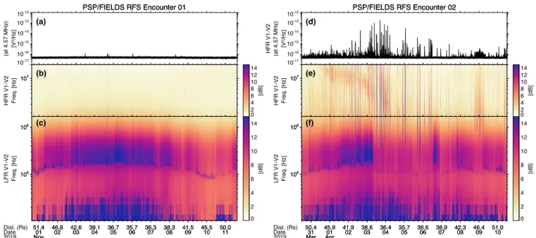
Inner Heliosphere Type III Bursts PSP/FIELDS RFS Encounter 01 PSP/FIELDS RFS Encounter 01 10-17 10-16 10-15 10-14 10-13 10-12 HFR V1-V2 (at 4.57 MHz) [V 2/Hz] 107 HFR V1-V2 Freq. [Hz] 107 0 2 4 6 8 10 12 14 [dB] 51.4 01 Nov 46.8 02 42.603 39.104 36.705 35.706 36.307 38.308 41.509 45.510 50.011 105 106 LFR V1-V2 Freq. [Hz] 51.4 01 Nov 46.8 02 42.603 39.104 36.705 35.706 36.307 38.308 41.509 45.510 50.011 105 106 0 2 4 6 8 10 12 14 [dB] Dist. (Rs) Date 2018 PSP/FIELDS RFS Encounter 02 PSP/FIELDS RFS Encounter 02 10-17 10-16 10-15 10-14 10-13 10-12 HFR V1-V2 (at 4.57 MHz) [V 2/Hz] 107 HFR V1-V2 Freq. [Hz] 107 0 2 4 6 8 10 12 14 [dB] 50.4 31 Mar 45.9 01 Apr 41.9 02 38.603 36.404 35.705 36.606 38.907 42.308 46.409 51.010 105 106 LFR V1-V2 Freq. [Hz] 50.4 31 Mar 45.9 01 Apr 41.9 02 38.603 36.404 35.705 36.606 38.907 42.308 46.409 51.010 105 106 0 2 4 6 8 10 12 14 [dB] Dist. (Rs) Date 2019 (a) (d) (b) (c) (f) (e)

Figure 1. Comparison of RFS observations from PSP Encounters 1 and 2. The two encounters were radically different in terms of radio emission, with Encounter 1 extremely quiet aside from a few small events, and Encounter 2 filled with numerous Type III radio bursts.

The absence of any significant radio activity is evident in the top two panels, which shows a cut through the

HFR spectrogram at 4.57 MHz (Fig. 1a) and the full

HFR spectrogram (Fig. 1b). The several small peaks

which are visible in Fig. 1a correspond to a few weak

Type III radio bursts and intervals of Jovian emission which occurred during E01.

The bottom panel shows the full LFR spectrogram

(Fig. 1c). At frequencies up to several hundred kHz,

the LFR spectrogram is dominated by the in situ signals

from shot noise and quasi-thermal noise (QTN) (

Meyer-Vernet & Perche 1989). The QTN feature at ∼90-150

kHz is the plasma peak, which allows RFS to make an

accurate absolute determination of fpeand therefore the

total electron density. The prominence of the plasma peak depends on the ratio of Debye length to antenna length, and for the 2 m FIELDS antennas the peak is

well resolved when fpe& 90 kHz. For a detailed analysis

of the QTN spectrum during the first two PSP

encoun-ters, seeMoncuquet et al.(2020).

Also visible in the LFR spectrogram are low frequency waves (observed from 10-30 kHz in LFR) which are

cor-related with near-fce waves observed at lower

frequen-cies (Malaspina et al. 2020), and large amplitude

electro-static Langmuir waves near the plasma frequency, which are evidence for electron beams in the inner heliosphere

(Bale et al. 2020).

The right panels of Figure1show the same data

prod-ucts for E02. During E02, the sun was much more active than during E01, as is apparent in the HFR time

se-ries (1d) and spectrogram (1e). In radio, the E02 solar

activity is dominated by Type III radio bursts, which are the strongest emissions in the HFR frequency range. Multiple Type IIIs occurred on a daily basis through-out E02, reaching a peak in intensity during ∼April 3-4.

As in E01, the LFR spectrum in E02 (1f) shows the

plasma line and electrostatic waves. The drop in den-sity on April 3 is consistent with measurements from

the SWEAP electron and ion detectors (Halekas et al.

2020).

After E02, a separate, nearly-continuous storm of ra-dio bursts lasting many days occurred in mid to late April, with the most intense period on April 16-19. Dur-ing this storm interval, the PSP spacecraft had daily contacts with the NASA Deep Space Network (DSN), for transmission of encounter data the ground. While the spacecraft is transmitting data, the instruments are turned off, so the PSP observations of this burst storm contain large daily data gaps. This interval is discussed

further in Sections4and5.

The spectrogram panels in Figure 1 are presented in

units of dB above background. This presentation was

chosen (rather than presenting the data in the V2_/Hz

units of spectral density) to facilitate the display of large Type III signals without erasing faint features like the plasma line and weak radio bursts, and to avoid the spectrogram color scale being dominated by the shot noise spectrum in the LFR. The background measure-ment used to produce the plot is based on spectra ob-served during a quiet period on 2018 October 6-7. This background spectrum, as well as several example spectra

(5)

from intervals during E01 and E02, is shown in Figure

2.

Figure 2a shows spectra from several quiet intervals

observed during E01. The falling, approximately power law spectrum which predominates in the LFR frequency range is a combination of shot noise and QTN. Each

E01 interval shown in Fig. 2a is an average of all RFS

Channel 0 (V1-V2) auto spectra observed over 1 hour of undisturbed solar wind, with no large fluctuations in density and no noticeable radio emission. The small rise in each spectrum at & 100 kHz is the plasma peak. Both the level of the shot noise/QTN spectrum and the frequency of the plasma peak increase with increasing density as PSP approaches close to the Sun.

In the HFR frequency range, the shot noise/QTN sig-nal decreases below the sigsig-nal from the galactic

syn-chrotron spectrum (Novaco & Brown 1978), which is the

smallest signal measured by the RFS and is on the same order as the RFS preamp/receiver input noise. The level of the galactic synchrotron spectrum enables an accurate measurement of the effective antenna length for

space-craft radio receivers (Eastwood et al. 2009; Zaslavsky

et al. 2011). Preliminary calibrations for the RFS

indi-cate an effective length of ∼3 m when the crossed dipole antennas (V1-V2 and V3-V4) are used as inputs to the two RFS channels.

Figure2b shows several shorter intervals (1-3 minutes)

during the more active E02, on April 3. The spectra are

less smooth than those in2a due to the shorter

averag-ing intervals. One interval, from 16:35-16:38, shows a

similar undisturbed profile as those shown in 2a. The

other spectra are taken during a typical large radio burst observed during Encounter 2. As seen at 1 AU, peak

ra-dio intensity occurs at frequencies of ∼ 1 MHz (Krupar

et al. 2014b). Detailed comparison of radio burst

inten-sity profiles in the inner heliosphere to those observed at 1 AU is beyond the scope of this work, but is likely to be a fruitful area of research as PSP approaches closer to the Sun–especially when the launch of Solar Orbiter adds another point to the available observations.

In Figure 2, the frequency coverage of the LFR and

HFR data products is shown below the spectra. The lowest frequency bin in LFR is not shown, since it is

dominated by the plasma waves described byMalaspina

et al.(2020) which vary over the averaging intervals used

in the figure. Several of the highest HFR frequency bins above 16 MHz are also not included, since they contain some aliased power from above the Nyquist frequency of 19.2 MHz.

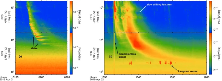
Figure 3 shows examples of events observed by RFS

during Encounter 2. The burst observed on April 1,

shown in Fig. 3a, is a Type IIIb burst, featuring

frequency structures known as striae (de La Noe &

Boischot 1972). The striae are associated with density

inhomogeneities in the source region of the burst (

Kon-tar et al. 2017; Sharykin et al. 2018). Fig. 3b shows

a large amplitude, event observed on April 2, with

slowly drifting Type II-like features from ∼5–10 MHz. The vertical feature near the start of the event is dis-persionless, to the time resolution of the measurement, and extends below the local plasma frequency, indicat-ing that it cannot be freely propagatindicat-ing radio emission. We suggest that this dispersionless signal corresponds to a change in the relative floating voltage of the an-tennas and spacecraft (and therefore system gain) due to photoemission from the impulsive UV emission

as-sociated with the source flare. Electrostatic Langmuir

waves are observed near the plasma frequency and could possibly be associated with the radio burst–however, we note that PSP frequently observes Langmuir waves in the inner heliosphere in the absence of radio emission

(Bale et al. 2020).

Before proceeding to detailed analysis of the radio bursts observed in E02, we note some limitations to these initial results. The calibration of the antenna ef-fective vectors has not yet been completed, so we present

results in units of power spectral density (PSD), V2/Hz,

rather than physical units of sfu or W/m2_/Hz.

How-ever, on-orbit measurements during spacecraft maneu-vers have indicated that the RFS receiver is sufficiently sensitive for observations of the galactic synchrotron spectrum, making an accurate absolute calibration in

the manner of Eastwood et al. (2009) and Zaslavsky

et al.(2011) possible.

We also note that in the statistical analysis presented in the following section, the measured PSD for observed

bursts has been radially scaled by a factor of (R/R0)2,

where R0 = 35.7R is the perihelion radius and R is

the radial distance of PSP from the sun. This rough scaling gives a first order correction to allow for

com-parison of burst amplitudes over the encounter. For

the radial distance range shown in Figure 1, this is a

factor of ∼2 between the closest and most distant

sam-ples in the spectrogram ((54 R/37.5 R)2). A more

accurate scale factor would correct for the radial dis-tance of the emission, which over the frequency range of 1–16 MHz corresponds to radial distances of 1.6–5

R (Leblanc et al. 1998). This second order correction

could increase or decrease the observed amplitude rela-tive to the source amplitude, depending on the location of the radio emission. As the PSP perihelion distance decreases throughout the mission, the importance of this correction will increase, and will likely require detailed goniopolarimetric/direction finding analysis for

(6)

determi-Inner Heliosphere Type III Bursts

Example RFS spectra from Encounter 01

10 kHz 100 kHz 1 MHz 10 MHz 10-17 10-16 10-15 10-14 10-13 10-12 Auto PSD V1-V2 [V 2/Hz] LFR HFR 2018-11-04 04:00-05:00 2018-11-02 16:00-17:00 2018-11-01 04:00-05:00 Bkgd. (2018 Oct 06-07)

Example RFS spectra from Encounter 02

10 kHz 100 kHz 1 MHz 10 MHz 10-17 10-16 10-15 10-14 10-13 10-12 Auto PSD V1-V2 [V 2/Hz] LFR HFR 2019-04-03 16:35-16:38 2019-04-03 16:50-16:51 2019-04-03 16:52-16:54 2019-04-03 16:57-17:00 Bkgd. (2018 Oct 06-07) (a) (b)

Figure 2. Example RFS spectra from the first two PSP encounters. The left plot, from Encounter 1, shows typical quiet time RFS auto spectra, displaying the shot noise spectrum and the plasma peak in the LFR frequency range, and the galactic radio background in the HFR range. The Encounter 2 plot on the right shows typical spectra observed during a Type III radio burst.

107 RFS HFR V1-V2 Freq. [Hz] 107 10-16 10-15 PSD [V 2/Hz] 0155 0200 0205 105 106 RFS LFR V1-V2 Freq. [Hz] 0155 0200 0205 105 106 10-16 10-15 PSD [V 2/Hz] hhmm 2019 Apr 01 107 RFS HFR V1-V2 Freq. [Hz] 107 10-16 10-15 10-14 PSD [V 2/Hz] 1530 1540 1550 1600 105 106 RFS LFR V1-V2 Freq. [Hz] 1530 1540 1550 1600 105 106 10-16 10-15 10-14 PSD [V 2/Hz] hhmm 2019 Apr 02 (a) (a) (b) striae dispersionless signal Langmuir waves slow drifting features

Figure 3. Examples of radio bursts observed during PSP Encounter 2. The left plot (a) shows a Type III with striations due to density fluctuations, and the right plot (b) shows a strong event with a vertical (dispersionless) signal near the start and slowly-drifting Type II-like features.

nation of the source location (Cecconi et al. 2008;

Kru-par et al. 2014a).

Due to these limitations of the current data set, in this work we restrict analysis to quantities (power law indices, waiting time distribution, and relative polariza-tion) that do not depend on absolute determination of amplitude.

4. STATISTICS OF TYPE III RADIO BURSTS

DURING E02

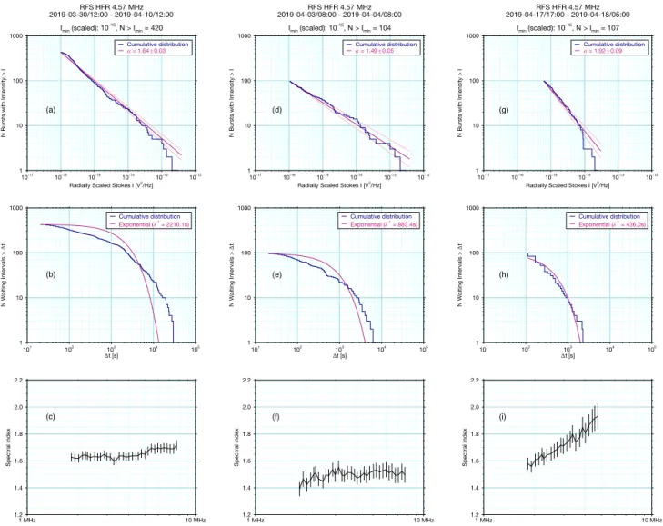
Figure 4 shows some basic statistical parameters of

Type III radio bursts observed during E02. Three time

intervals are presented: in the first column (Figure4

a-c), statistics are shown for the entire encounter, using

the same time range as in Figure1. The second column

covers a single 24 hour period from 2019 April 03/08:00 to 2019 April 04/08:00, which was the most intense pe-riod of radio burst activity during E02. The final column covers an interval during the mid-April Type III storm, when the RFS instrument was turned on and making

ob-servations at a reduced cruise mode rate. Figure6shows

HFR observations during this portion of the storm. Individual bursts were detected in the RFS spectro-grams by identifying maxima in cuts through the

(7)

spec-trogram at a given frequency. Bursts were required to be above a threshold value to eliminate random fluctua-tions, the effects of high frequency electron thermal noise

(Maksimovic et al. 2020), and observed Jovian emission.

For all analyzed intervals, a minimum scaled PSD of

Imin= 10−16V2/Hz was used as a threshold. To

calcu-late intensity I, we used the sum of the V 1 − V 2 and V 3 − V 4 cross dipoles.

A lower threshold for I would result in a count of & 1000 Type III radio bursts observed during E02, but would be contaminated by some non-Type III sources

described above. Above the threshold, there are 420

bursts during the 11 days of E02, 104 bursts during the most intense 24 hour period on April 3/08:00 to April 4/08:00, and 107 during the 12 hour segment of the Type III storm from April 17/17:00 to April 18/05:00.

The top panels of Figure 4 show the distribution of

PSD for all bursts > Imin at a sample HFR frequency

of 4.57 MHz. Following the technique used in (

East-wood et al. 2010), we plot the cumulative distribution

of burst intensity I and calculate a power law index α using the maximum likelihood method. From an

inten-sity distribution f (I) ∝ I−α_{, α and σ}

αcan be computed

as (Wheatland 2004):

α = N

ΣN

i=1ln(Ii/Imin)

+ 1 (1)

σα≈ (α − 1)N1/2 (2)

In the cumulative distribution plots shown in Fig.

4(a,d,g), a power law index of α corresponds to a slope

of −α + 1. For each interval, the intensity

distribu-tion follows a power law reasonably well within the

expected uncertainty. The power law index is

flat-test (α = 1.49 ± 0.05) during the time period of the

most intense bursts (Figure4d), somewhat steeper (α =

1.64 ± 0.03) over the entire encounter (Figure 4a), and

steepest (α = 1.92 ± 0.03) during the burst storm

(Fig-ure 4g). The power law index during the storm agrees

reasonably well with the index of 2.10±0.05 observed by

Eastwood et al.(2010) at 5.025 MHz, while the steeper

index observed during the non-storm encounter period

agrees with the index of 1.69 found byFitzenreiter et al.

(1976).

Cumulative waiting time distributions are shown in

Figure4(b,e,h). For reference, a model waiting time

dis-tribution curve corresponding to a simple Poisson pro-cess is plotted along with the cumulative distributions. This model is given by:

N (twait> ∆t) ∝ exp−λ∆t (3)

where λ is the rate of occurrence of bursts during the interval. The Type III storm interval appears to be con-sistent with a single continuous Poisson process, while the waiting time distributions during encounter display more structure, corresponding to distinct intervals of dif-ferent activity. A Bayesian block analysis of the type

performed by Eastwood et al. (2010) could be used to

separate sub-intervals during the encounter, with each distinct sub-interval associated with an independent rate of burst activity.

The variation of spectral index α with frequency is

shown in Figure 4(c,f,i). We have limited the

fre-quency range in these plots to f < 8 MHz, because there is an intermittent source of noise (possibly instru-ment or spacecraft-generated) which occurs sporadically throughout the encounter for a single spectra measure-ment at frequencies above 8 MHz. In the case of the Type III storm, we have further limited our analysis to below 5 MHz, because above 5 MHz the radio bursts have a duration lower than the cadence of the obser-vations. We also limit the frequency range to f > 1.8 MHz, to avoid the effects of the high frequency tail of the QTN spectrum during encounter.

During the encounter period the spectral index re-mained at α ∼ 1.6 − 1.7 from 1.8 − 8 MHz, with a possible steepening at higher frequencies. During the 24 hour peak intensity period, the spectral index was slightly lower at α ∼ 1.4 − 1.5, and nearly constant over the entire frequency range. In contrast, and also in

con-trast to the storm analyzed byEastwood et al.(2010),

the late April storm becomes steeper with increasing frequency, from α ∼ 1.6 at 1.8 MHz to α ∼ 1.9 at 8 MHz.

Variation in α with frequency may be due to the lo-cation of the active region relative to the spacecraft, the

refraction of emitted radiation (Thejappa et al. 2012),

and scattering of the emission as it propagates.

Multi-point measurements of directivity patterns (Lecacheux

et al. 1989;Bonnin et al. 2008;Reiner et al. 2009), and

the study of many burst intervals will be useful in de-termining why some periods exhibit no variation of α

with frequency (Eastwood et al. (2010), the encounter

periods analyzed here) and some periods exhibit definite

trends (Fitzenreiter et al.(1976), the late April storm

analyzed in this paper).

5. POLARIZATION OF TYPE III RADIO BURSTS

In this section, we describe the circular polarization observed for a subset of radio bursts during E02. The analysis in the previous section employed the Stokes in-tensity (I) parameter. From the RFS auto and cross spectra products, it is also possible to calculate the

(8)

Inner Heliosphere Type III Bursts 1 MHz 10 MHz 1.2 1.4 1.6 1.8 2.0 2.2 Spectral index 1 MHz 10 MHz 1.2 1.4 1.6 1.8 2.0 2.2 Spectral index 1 MHz 10 MHz 1.2 1.4 1.6 1.8 2.0 2.2 Spectral index 101 ₁₀2 ₁₀3 ₁₀4 ₁₀5 Dt [s] 1 10 100 1000 N Waiting Intervals > D t Cumulative distribution Exponential (l-1_{= 2210.1s)} 101 ₁₀2 ₁₀3 ₁₀4 ₁₀5 Dt [s] 1 10 100 1000 N Waiting Intervals > D t Cumulative distribution Exponential (l-1_{= 883.4s)} 101 ₁₀2 ₁₀3 ₁₀4 ₁₀5 Dt [s] 1 10 100 1000 N Waiting Intervals > D t Cumulative distribution Exponential (l-1_{= 436.0s)} RFS HFR 4.57 MHz 2019-03-30/12:00 - 2019-04-10/12:00 Imin (scaled): 10-16_{, N > Imin = 420}

10-17 ₁₀-16 ₁₀-15 ₁₀-14 ₁₀-13 ₁₀-12

Radially Scaled Stokes I [V2_/Hz]

1 10 100 1000

N Bursts with Intensity > I

Cumulative distribution a = 1.64±0.03

RFS HFR 4.57 MHz 2019-04-03/08:00 - 2019-04-04/08:00

Imin (scaled): 10-16_{, N > Imin = 104}

10-17 ₁₀-16 ₁₀-15 ₁₀-14 ₁₀-13 ₁₀-12

1 10 100 1000

Cumulative distribution a = 1.49±0.05

RFS HFR 4.57 MHz 2019-04-17/17:00 - 2019-04-18/05:00

Imin (scaled): 10-16_{, N > Imin = 107}

10-17 ₁₀-16 ₁₀-15 ₁₀-14 ₁₀-13 ₁₀-12

1 10 100 1000

Cumulative distribution a = 1.92±0.09 (a) (b) (c) (d) (e) (f) (g) (h) (i)

Figure 4. Statistics of Type III radio burst occurrence during and after PSP Encounter 2. The three columns show statistics for an interval covering all of Encounter 2 (a-c), the 24 hours showing the most intense burst activity (d-f), and a post-encounter interval during a Type III storm (g-i). Each column shows the distribution of burst intensity (top), the waiting time distribution (center), and the variation in power law index α with frequency (bottom).

Stokes Q, U , and V parameters, representing the lin-ear (Q, U ) and circular (V ) polarization:

I = V12V12∗ + V34V34∗ (4)

Q = V12V12∗ − V34V34∗ (5)

U = V12V34∗ + (V12V34∗)∗ (6)

iV = V12V34∗ − (V12V34∗)

∗ ₍₇₎

where V12V12∗ and V34V34∗ are the RFS auto spectra

from the V 1 − V 2 and V 3 − V 4 channels, and V12V34∗ is

the RFS cross spectrum. Note that we use the conven-tion where right-hand circular (RHC) polarizaconven-tion in-dicates an electric field vector rotating clockwise when viewed from the radio source in the direction of

propaga-tion towards the spacecraft. In Equapropaga-tion7, V < 0

corre-sponds to RHC polarization. Although we can in princi-ple calculate all Stokes polarization parameters, we only present V here because the linear polarization Stokes

parameters are affected by Faraday rotation (Suzuki &

Dulk 1985) so any source linear polarization (U , Q) is

unlikely to be measurable remotely.

In general, calculation of the Stokes parameters re-quires correction by the Mueller matrix, which compen-sates for instrumental effects on observed polarization

of radio sources (e.g. Heiles et al. 2001). For the case

of short dipole antennas such as the 2 m FIELDS an-tennas, the effective length vectors of the antennas are real-valued and this correction is substantially simplified

(Lecacheux 2011). Under the assumption that the true

linear polarization of the Type III emission is negligible, and noting that Q ≈ U ≈ 0 during the burst intervals

(9)

where circular polarization V was observed, Equation 6

of Lecacheux (2011) shows that a simple computation

of relative circular polarization (V /I) is approximately valid even without detailed consideration of arrival di-rection or cordi-rections for antenna non-orthogonality.

5.1. Polarization of individual radio bursts observed near perihelion

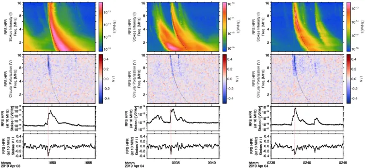
Figure5shows I and V /I spectrograms and time

pro-files (at 10 MHz) for three radio bursts exhibiting cir-cular polarization (out of seven bursts identified in E02 with clear signatures of circular polarization). In each burst, RHC polarization is present for a short time near the leading edge of the burst, at frequencies above ∼6

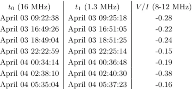
MHz. Table1 presents the time of the leading edge of

the burst near the top and bottom of the HFR range (t0

and t1), and the fraction of circular polarization V /I,

observed for each of the seven individual bursts ana-lyzed in this study. In addition to the seven bursts an-alyzed here, numerous other bursts presented weaker, marginally distinguishable signals. For example, in

Fig-ure 5, the weaker Type IIIs starting at approximately

00:35:30 and 02:41:00 display faint possible signals of circular polarization. t0 (16 MHz) t1 (1.3 MHz) V /I (8-12 MHz) April 03 09:22:38 April 03 09:25:18 -0.28 April 03 16:49:26 April 03 16:51:05 -0.22 April 03 18:49:04 April 03 18:51:25 -0.24 April 03 22:22:59 April 03 22:25:14 -0.15 April 04 00:34:14 April 04 00:36:48 -0.19 April 04 02:38:10 April 04 02:40:30 -0.38 April 04 05:35:04 April 04 05:37:23 -0.16

Table 1. Time and circular polarization for seven radio

bursts observed during Encounter 2. The times t0 and t1

correspond to the times of the leading edge of the radio burst. The dotted frequency profiles shown in Figure5are derived from these times.

5.2. Polarization of Type III storm

As mentioned in previous sections, a days-long Type III storm was observed by RFS during mid-late April. At this time, the FIELDS instruments were in cruise mode, recording spectra approximately once per 56

sec-onds. An example interval is shown in Figure 6.

Un-like any of the active periods observed during the en-counter, this storm exhibited significant circular polar-ization throughout the storm period, associated with nearly every observed burst. As in the bursts observed during encounter, the polarized emission is overwhelm-ingly in the RHC sense. The average degree of

polariza-tion increases slightly with frequency, from about −0.1 at 1 MHz to −0.2 at 5 MHz (above 5 MHz, the cruise mode cadence is too slow to clearly distinguish individ-ual bursts).

5.3. Analysis of Polarization Observations

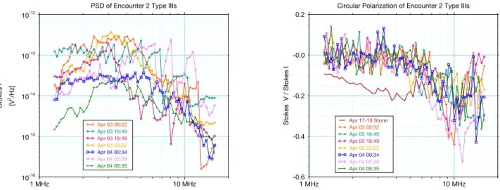
Figure7shows profiles of Stokes intensity I and

circu-lar pocircu-larization V /I for the bursts in Table1. The

pro-files are based on cuts through the spectrogram plots at

the times defined in Table1, which are shown as dotted

lines in Figure 5. The intensity profiles are consistent

with typical Type III profiles observed at 1 AU (Krupar

et al. 2014b). It is not immediately apparent why only a

small fraction of bursts observed during E02 showed sig-natures of circular polarization. From comparing Figure

7with Figure4d, it is clear that the seven bursts

show-ing circular polarization are relatively high in amplitude. However, many comparably large bursts, including the

two examples in Figure3, did not show signs of

circu-lar pocircu-larization, and the small number of observations (N = 7) does not permit a detailed quantitative analy-sis of the relation between burst intensity and degree of polarization.

For each of the seven analyzed bursts, Stokes V /I in-creases from a value ∼0 below 4 MHz, to a value of −0.15 to −0.38 in the range from 8-12 MHz, indicating partial RHC polarization. This agrees reasonably well

with previous observations at higher frequencies (Dulk

& Suzuki 1980).

The circularly polarized component of these bursts

likely corresponds to fundamental (F ) emission at fpe,

and not harmonic (H) emission at 2fpe. Previous

stud-ies of Type III bursts at starting at slightly higher fre-quencies (> 24 MHz) are consistent with the values of

V /I in Table1assuming they correspond to the F

com-ponent, while the values of V /I for the H component

are lower (Dulk & Suzuki 1980).

For all bursts listed in Table 1, the maximum value

of circular polarization V /I precedes the maximum in-tensity I, and polarized signal is absent from the latter

stage of the burst (see Figure5). This is also consistent

with previous results (Dulk et al. 1998) showing that

the initial phase of radio bursts is dominated by funda-mental emission, which is more strongly polarized than harmonic emission. After the initial period (i.e. at the peak and during the exponential decay of the burst), emission may be from the fundamental or harmonic. If this later part of the burst is dominated by harmonic emission, then the weaker polarization signal is natu-rally explained by the weaker polarization observed in

the harmonic component of Type IIIs (Dulk et al. 1984).

(10)

Inner Heliosphere Type III Bursts 2 4 8 16 RFS HFR

Stokes Intensity (I)

Freq. [MHz] 2 4 8 16 10-16 10-15 10-14 10-13 I [V 2/Hz] 2 4 8 16 RFS HFR Circular Polarization (V) Freq. [MHz] 2 4 8 16 -0.4 -0.2 0.0 0.2 0.4 V / I 10-17 10-16 10-15 10-14 10-13 RFS HFR (at 10 MHz) Stokes I [V2/Hz] 0235 0240 0245 -0.4 -0.20.0 0.2 0.4 RFS HFR (at 10 MHz) Stokes V / I hhmm 2019 Apr 04 10-17 10-16 10-15 10-14 10-13 RFS HFR (at 10 MHz) Stokes I [V2/Hz] 0235 0240 0245 -0.4 -0.20.0 0.2 0.4 RFS HFR (at 10 MHz) Stokes V / I hhmm 2019 Apr 04 2 4 8 16 RFS HFR

Freq. [MHz] 2 4 8 16 10-16 10-15 10-14 10-13 I [V 2/Hz] 2 4 8 16 RFS HFR Circular Polarization (V) Freq. [MHz] 2 4 8 16 -0.4 -0.2 0.0 0.2 0.4 V / I 10-17 10-16 10-15 10-14 10-13 10-12 RFS HFR (at 10 MHz) Stokes I [V2/Hz] 1650 1655 -0.4 -0.20.0 0.2 0.4 RFS HFR (at 10 MHz) Stokes V / I hhmm 2019 Apr 03 10-17 10-16 10-15 10-14 10-13 10-12 RFS HFR (at 10 MHz) Stokes I [V2/Hz] 1650 1655 -0.4 -0.20.0 0.2 0.4 RFS HFR (at 10 MHz) Stokes V / I hhmm 2019 Apr 03 2 4 8 16 RFS HFR

Stokes Intensity (I) Freq. [MHz] ₂

4 8 16 10-16 10-15 10-14 10-13 I [V 2/Hz] 2 4 8 16 RFS HFR Circular Polarization (V) Freq. [MHz] 2 4 8 16 -0.4 -0.2 0.0 0.2 0.4 V / I 10-17 10-16 10-15 10-14 RFS HFR (at 10 MHz) Stokes I [V2/Hz] 0035 0040 -0.4 -0.20.0 0.2 0.4 RFS HFR (at 10 MHz) Stokes V / I hhmm 2019 Apr 04 10-17 10-16 10-15 10-14 RFS HFR (at 10 MHz) Stokes I [V2/Hz] 0035 0040 -0.4 -0.20.0 0.2 0.4 RFS HFR (at 10 MHz) Stokes V / I hhmm 2019 Apr 04

Figure 5. Example radio bursts displaying circular polarization above ∼6 MHz. In each plot, the top panel shows the Stokes intensity (I), while the second panel shows the relative circular polarization Stokes V /I. Negative V , in blue, indicates right hand circular polarization. In each spectrogram plot, the dotted line indicates the time profile of the leading edge of the burst. The bottom two panels show time profiles of I and V /I at a frequency of 10 MHz, showing how the polarization is localized near the leading edge of the burst and is absent at later times. The time of maximum circular polarization is indicated in these panels with a red dotted line.

2 4 8 16

RFS HFR

Freq. [MHz] 2 4 8 16 RFS HFR

Freq. [MHz] 2 4 8 16 2 4 8 16 2 4 8 16 2 4 8 16 2 4 8 16 2 4 8 16 2 4 8 16 2 4 8 16 2 4 8 16 2 4 8 16 10-16 10-15 10-14 I [V 2/Hz] 1600 Apr 17 2000 Apr 180000 0400 2 4 8 16 RFS HFR Circular Polarization (V ) Freq. [MHz] 1600 Apr 17 2000 Apr 180000 0400 2 4 8 16 RFS HFR Circular Polarization (V ) Freq. [MHz] 1600 Apr 17 2000 Apr 180000 0400 2 4 8 16 RFS HFR Circular Polarization (V ) Freq. [MHz] 1600 Apr 17 2000 Apr 180000 0400 2 4 8 16 RFS HFR Circular Polarization (V ) Freq. [MHz] 1600 Apr 17 2000 Apr 180000 0400 2 4 8 16 RFS HFR Circular Polarization (V ) Freq. [MHz] 1600 Apr 17 2000 Apr 180000 0400 2 4 8 16 RFS HFR Circular Polarization (V ) Freq. [MHz] 1600 Apr 17 2000 Apr 180000 0400 2 4 8 16 RFS HFR Circular Polarization (V ) Freq. [MHz] 1600 Apr 17 2000 Apr 180000 0400 2 4 8 16 RFS HFR Circular Polarization (V ) Freq. [MHz] 1600 Apr 17 2000 Apr 180000 0400 2 4 8 16 RFS HFR Circular Polarization (V ) Freq. [MHz] 1600 Apr 17 2000 Apr 180000 0400 2 4 8 16 RFS HFR Circular Polarization (V ) Freq. [MHz] 1600 Apr 17 2000 Apr 180000 0400 2 4 8 16 1600 Apr 17 2000 Apr 180000 0400 2 4 8 16 1600 Apr 17 2000 Apr 180000 0400 2 4 8 16 1600 Apr 17 2000 Apr 180000 0400 2 4 8 16 1600 Apr 17 2000 Apr 180000 0400 2 4 8 16 1600 Apr 17 2000 Apr 180000 0400 2 4 8 16 1600 Apr 17 2000 Apr 180000 0400 2 4 8 16 1600 Apr 17 2000 Apr 180000 0400 2 4 8 16 1600 Apr 17 2000 Apr 180000 0400 2 4 8 16 1600 Apr 17 2000 Apr 180000 0400 2 4 8 16 -0.4 -0.2 0.0 0.2 0.4 V / I hhmm 2019

Figure 6. Type III storm with circular polarization. Like the individual events in the previous section, the sense of the polarization is RHC.

fundamental, then the initially polarized signal could be affected by scattering in the inner heliosphere. A recent

study by Krupar et al. (2018) simulated the time

pro-file propro-file of Type IIIs based on a Monte Carlo model, concluding that the exponential decay of the intensity profile could be explained by small scale density fluc-tuations. The same scattering process could reduce the coherence of an initially circularly polarized signal, leav-ing the latter part of the burst unpolarized as measured by the observer.

Previous observations have established a correlation with the sense of circular polarization (for Type I and

Type III bursts) and the polarity of the leading sunspot in the active region associated with the radio emission

(Dulk et al. 1984; Stewart 1985; Reiner et al. 2007).

This is consistent with the SDO/HMI magnetograms during the month of April, which show the active re-gion (NOAA 12738) in the Northern hemisphere, with a leading spot with negative polarity (field pointing into the Sun) and a trailing spot with positive polarity (field pointing out from the Sun).

6. DISCUSSION

A major reason that the polarization of Type III radi-ation is of interest is that it provides a remote probe of the coronal magnetic field, where the degree of circular polarization is dependent on the strength of the field. In the case of harmonic emission, theory predicts a direct relation between the degree of polarization and the ra-tio of electron gyrofrequency and the plasma frequency,

V /I ∼ A(fB/fp) (Dulk et al. 1984). This relation was

used by Reiner et al. (2007) to infer the profile of the

coronal magnetic field, and compare to model coronal

fields (Dulk & McLean 1978).

The polarization of the fundamental component is less straightforward, but also depends on the properties of the coronal field. Magnetoionic theory predicts that fun-damental emission is generated with 100% polarization in the o-mode, which is observed in Type I radio bursts

(11)

PSD of Encounter 2 Type IIIs 1 MHz 10 MHz 10-16 10-15 10-14 10-13 10-12 Stokes I 2 [V/Hz] Apr 03 09:22 Apr 03 16:49 Apr 03 18:49 Apr 03 22:22 Apr 04 00:34 Apr 04 02:38 Apr 04 05:35

Circular Polarization of Encounter 2 Type IIIs

1 MHz 10 MHz -0.6 -0.4 -0.2 -0.0 0.2

Stokes V / Stokes I Apr 17-19 Storm

Apr 03 09:22 Apr 03 16:49 Apr 03 18:49 Apr 03 22:22 Apr 04 00:34 Apr 04 02:38 Apr 04 05:35

Figure 7. Stokes I and V /I profiles of Type III radio bursts observed during PSP Encounter 2. For each individual burst, the profiles are derived from a frequency-dependent cut through the spectrogram, as shown in Figure5. The average V /I for the storm period shown in Figure6is shown along with the individual cuts.

(Melrose 2017). However, for Type III radio bursts,

100% polarization is not observed, which implies that some depolarization mechanism must be in effect to re-duce the completely polarized emission to the lower

lev-els observed. Melrose (2006) has proposed reflection as

a mechanism, with emission created in regions of lower density (ducts) surrounded by regions of higher density. The radio emission would reflect off the duct boundaries, and in the process become depolarized. An alternative

explanation was proposed byKim et al.(2007), who

de-veloped theory and simulations to show that, under con-ditions consistent with solar wind observations, emission can be generated partially in the o mode and partially in the x mode. Direct generation of emission in different modes could account for the observed <100% polariza-tion without need for a depolarizapolariza-tion mechanism.

6.1. Comparison with previous spacecraft measurements

As discussed previously, partial circular polarization has been observed from the ground, but previous space-craft measurements have not reported polarization sig-natures at frequencies greater than a few MHz. The rea-son why RFS observes polarization at frequencies & 6 MHz is most likely not due to observing position or any

particular antenna or spacecraft geometry. Although

the intensity (in sfu or W/m2/Hz) for a given burst is

higher in the inner heliosphere, the 2 m PSP antennas are considerably shorter than previous radio instruments

such as STEREO (Bougeret et al. 2008) (6 m triaxial

an-tennas) or Wind (Bougeret et al. 1995) (100 m and 15 m

tip to tip dipoles in the spin plane, and 12 m in the axial

direction). Therefore, the signal to noise ratio is not sig-nificantly higher for PSP than for previous spacecraft, at least not during the initial encounters. The cross dipole configuration of PSP is convenient for simple computa-tion of Stokes parameters as presented in this work, but both Wind and STEREO are fully capable of making goniopolarimetric measurements of source polarization

(Fainberg et al. 1985;Cecconi et al. 2008;Krupar et al.

2014a).

The most likely reason that similar signatures of po-larized Type III bursts have not been reported using STEREO or Wind data is the relatively slow cadence of the radio measurements. For STEREO/WAVES HFR, the cadence is typically ∼40 seconds, likely too short to measure the circular polarization, which typically only appears in the RFS data for 1-3 spectra at 7 second cadence. For Wind, the relevant frequency range is cov-ered by the RAD2 receiver, which typically makes mea-surements at ∼16 seconds, which could be marginal for

short-lasting circular polarization observations.

How-ever, direction finding mode for RAD2, which is required for measuring polarization, is not always enabled.

6.2. Absence of Associated in situ Electron Observations

As of the time of writing, there were no observations of in situ electron beams associated with any of the Type III radio bursts in E02, of the type that have been

pre-viously observed by other spacecraft (Lin et al. 1981;

Ergun et al. 1998). This is likely due to the magnetic

connectivity of PSP during E02. The active region likely responsible for the bursts (NOAA 12738) was in the

(12)

Inner Heliosphere Type III Bursts northern hemisphere, while during the encounter the

ra-dial component of the magnetic field Br was

predomi-nantly negative, indicating connection to the Sun on the southward side of the heliospheric current sheet.

Additionally, the instrument configuration on PSP for the first two encounters was not ideal for detection of the several to ∼10 keV electron beams which generate Lang-muir waves. This energy range is below the minimum

energies of the ISOIS electron detectors (McComas et al.

2016), and the SWEAP electron electrostatic analyzers

were configured with a maximum energy of 2 keV. In fu-ture encounters, the maximum SWEAP energy could be extended (although at the expense of cadence or energy resolution).

The PSP perihelion distance will decrease throughout the course of the mission, eventually reaching closest

ap-proach of of 9.86 Rin 2024. At that time, the Sun is

ex-pected to be at or near the maximum of the solar cycle, and conditions will be ripe for detection of a in situ Type III in the inner heliosphere (ideally with electron beams in the key energy range). The in situ measurements made during such an event will provide observational tests of proposed theories of radio emission. As an ex-ample, the in situ density measurements in the inner he-liosphere could show evidence of the ducting structures

proposed by Melrose (2006), and high cadence

wave-forms recorded by the FIELDS Time Domain Sampler

(TDS) instrument could measure emission wave modes directly from within a radio burst source region, to test

against the predictions ofKim et al.(2007). These inner

heliospheric measurements, combined with other ground and space-based radio observations (including Solar Or-biter after 2020) will offer new fundamental insights into the nature of solar radio emission.

ACKNOWLEDGMENTS

The FIELDS experiment on the Parker Solar Probe spacecraft was designed and developed under NASA contract NNN06AA01C. The FIELDS team acknowl-edges the extraordinary contributions of the Parker So-lar Probe mission operations and spacecraft engineer-ing teams at the Johns Hopkins University Applied Physics Laboratory. The RFS science team is immensely grateful to Dennis Seitz and Dorothy Gordon for their contributions to the analog and digital design of the RFS receiver. MP acknowledges useful discussions with Vratislav Krupar. SDB acknowledges the support of the Leverhulme Trust Visiting Professorship program. Data access and processing was performed using SPEDAS

(Angelopoulos et al. 2019). PSP/FIELDS data is

pub-licly available athttp://fields.ssl.berkeley.edu/data/.

REFERENCES

Angelopoulos, V., Cruce, P., Drozdov, A., et al. 2019,

SSRv, 215, 9, doi:10.1007/s11214-018-0576-4

Bale, S. D., Goetz, K., Harvey, P. R., et al. 2016, SSRv, 204, 49, doi:10.1007/s11214-016-0244-5

Bale, S. D., Pulupa, M., Goetz, K., et al. 2020, ApJ, this issue

Bonnin, X., Hoang, S., & Maksimovic, M. 2008, A&A, 489,

419, doi:10.1051/0004-6361:200809777

Bougeret, J. L., Kaiser, M. L., Kellogg, P. J., et al. 1995,

SSRv, 71, 231, doi:10.1007/BF00751331

Bougeret, J. L., Goetz, K., Kaiser, M. L., et al. 2008, SSRv, 136, 487, doi:10.1007/s11214-007-9298-8

Cecconi, B. 2019, arXiv e-prints, arXiv:1901.03599. https://arxiv.org/abs/1901.03599

Cecconi, B., Bonnin, X., Hoang, S., et al. 2008, SSRv, 136,

549, doi:10.1007/s11214-007-9255-6

de La Noe, J., & Boischot, A. 1972, A&A, 20, 55

Dulk, G. A., Leblanc, Y., Robinson, P. A., Bougeret, J.-L., & Lin, R. P. 1998, J. Geophys. Res., 103, 17223,

doi:10.1029/97JA03061

Dulk, G. A., & McLean, D. J. 1978, SoPh, 57, 279,

doi:10.1007/BF00160102

Dulk, G. A., & Suzuki, S. 1980, A&A, 88, 203

Dulk, G. A., Suzuki, S., & Sheridan, K. V. 1984, A&A, 130, 39

Eastwood, J. P., Bale, S. D., Maksimovic, M., et al. 2009,

Radio Science, 44, RS4012, doi:10.1029/2009RS004146

Eastwood, J. P., Wheatland, M. S., Hudson, H. S., et al.

2010, ApJL, 708, L95, doi:10.1088/2041-8205/708/2/L95

Ergun, R. E., Larson, D., Lin, R. P., et al. 1998, ApJ, 503, 435, doi:10.1086/305954

Fainberg, J., Hoang, S., & Manning, R. 1985, A&A, 153, 145

Fitzenreiter, R. J., Fainberg, J., & Bundy, R. B. 1976,

SoPh, 46, 465, doi:10.1007/BF00149870

Fox, N. J., Velli, M. C., Bale, S. D., et al. 2016, SSRv, 204, 7, doi:10.1007/s11214-015-0211-6

Ginzburg, V. L., & Zhelezniakov, V. V. 1958, Soviet Ast., 2, 653

Gurnett, D. A., & Anderson, R. R. 1976, Science, 194, 1159, doi:10.1126/science.194.4270.1159

Halekas, J. S., Whittlesey, P., Larson, D. E., et al. 2020, ApJ, this issue

(13)

Hanasz, J., Schreiber, R., & Aksenov, V. I. 1980, A&A, 91, 311

Heiles, C., Perillat, P., Nolan, M., et al. 2001, PASP, 113, 1274, doi:10.1086/323289

Kellogg, P. J. 1980, ApJ, 236, 696, doi:10.1086/157789 Kim, E.-H., Cairns, I. H., & Robinson, P. A. 2007, PhRvL,

99, 015003, doi:10.1103/PhysRevLett.99.015003

Kontar, E. P., Yu, S., Kuznetsov, A. A., et al. 2017, Nature Communications, 8, 1515,

doi:10.1038/s41467-017-01307-8

Krupar, V., Maksimovic, M., Santolik, O., Cecconi, B., & Kruparova, O. 2014a, SoPh, 289, 4633,

doi:10.1007/s11207-014-0601-z

Krupar, V., Maksimovic, M., Santolik, O., et al. 2014b, SoPh, 289, 3121, doi:10.1007/s11207-014-0522-x Krupar, V., Maksimovic, M., Kontar, E. P., et al. 2018,

ApJ, 857, 82, doi:10.3847/1538-4357/aab60f

Leblanc, Y., Dulk, G. A., & Bougeret, J.-L. 1998, SoPh,

183, 165, doi:10.1023/A:1005049730506

Lecacheux, A. 2011, in Planetary, Solar and Heliospheric Radio Emissions (PRE VII), ed. H. O. Rucker, W. S. Kurth, P. Louarn, & G. Fischer, 13–35

Lecacheux, A., Steinberg, J. L., Hoang, S., & Dulk, G. A. 1989, A&A, 217, 237

Lin, R. P., Potter, D. W., Gurnett, D. A., & Scarf, F. L. 1981, ApJ, 251, 364, doi:10.1086/159471

Maksimovic, M., Bale, S. D., Bercic, L., et al. 2020, ApJ, this issue

Malaspina, D. M., Halekas, J., Bercic, L., et al. 2020, ApJ, this issue

McComas, D. J., Alexander, N., Angold, N., et al. 2016,

SSRv, 204, 187, doi:10.1007/s11214-014-0059-1

Melrose, D. B. 2006, ApJ, 637, 1113, doi:10.1086/498499

—. 2017, Reviews of Modern Plasma Physics, 1, 5,

doi:10.1007/s41614-017-0007-0

Meyer-Vernet, N., & Perche, C. 1989, J. Geophys. Res., 94,

2405, doi:10.1029/JA094iA03p02405

Moncuquet, M., Meyer-Vernet, N., Issautier, K., et al. 2020, ApJ, this issue

Novaco, J. C., & Brown, L. W. 1978, ApJ, 221, 114,

doi:10.1086/156009

Pulupa, M., Bale, S. D., Bonnell, J. W., et al. 2017, Journal of Geophysical Research (Space Physics), 122, 2836,

doi:10.1002/2016JA023345

Reid, H. A. S., & Ratcliffe, H. 2014, Research in Astronomy and Astrophysics, 14, 773,

doi:10.1088/1674-4527/14/7/003

Reiner, M. J., Fainberg, J., Kaiser, M. L., & Bougeret, J. L. 2007, SoPh, 241, 351, doi:10.1007/s11207-007-0277-8 Reiner, M. J., Goetz, K., Fainberg, J., et al. 2009, SoPh,

259, 255, doi:10.1007/s11207-009-9404-z

Sasikumar Raja, K., & Ramesh, R. 2013, ApJ, 775, 38,

doi:10.1088/0004-637X/775/1/38

Sharykin, I. N., Kontar, E. P., & Kuznetsov, A. A. 2018,

SoPh, 293, 115, doi:10.1007/s11207-018-1333-2

Stewart, R. T. 1985, SoPh, 96, 381,

doi:10.1007/BF00149692

Suzuki, S., & Dulk, G. A. 1985, Bursts of type III and type V., ed. D. J. McLean & N. R. Labrum, 289–332

Thejappa, G., MacDowall, R. J., & Bergamo, M. 2012,

ApJ, 745, 187, doi:10.1088/0004-637X/745/2/187

Wheatland, M. S. 2004, ApJ, 609, 1134,

doi:10.1086/421261