Modelling photochemistry in alpine valleys

HAL Id: hal-00327852

https://hal.archives-ouvertes.fr/hal-00327852

HAL is a multi-disciplinary open access

archive for the deposit and dissemination of sci-entific research documents, whether they are pub-lished or not. The documents may come from teaching and research institutions in France or abroad, or from public or private research centers.

L’archive ouverte pluridisciplinaire HAL, est destinée au dépôt et à la diffusion de documents scientifiques de niveau recherche, publiés ou non, émanant des établissements d’enseignement et de recherche français ou étrangers, des laboratoires publics ou privés.

Modelling photochemistry in alpine valleys

G. Brulfert, C. Chemel, E. Chaxel, J. P. Chollet

To cite this version:

G. Brulfert, C. Chemel, E. Chaxel, J. P. Chollet. Modelling photochemistry in alpine valleys. Atmo-spheric Chemistry and Physics Discussions, European Geosciences Union, 2005, 5 (2), pp.1797-1828. �hal-00327852�

ACPD

Full Screen / Esc

Print Version Interactive Discussion

EGU

Atmos. Chem. Phys. Discuss., 5, 1797–1828, 2005 www.atmos-chem-phys.org/acpd/5/1797/

SRef-ID: 1680-7375/acpd/2005-5-1797 European Geosciences Union

Atmospheric Chemistry and Physics Discussions

Modelling photochemistry in alpine

valleys

G. Brulfert, C. Chemel, E. Chaxel, and J. P. Chollet

Laboratory of Geophysical and industrial Fluid Flows, University J. Fourier, INP Grenoble, CNRS, BP53, 38041 Grenoble cedex, France

Received: 1 July 2004 – Accepted: 7 December 2004 – Published: 21 March 2005 Correspondence to: G. Brulfert (guillaume.brulfert@hmg.inpg.fr)

ACPD

Full Screen / Esc

Print Version Interactive Discussion

EGU

Abstract

Road traffic is a serious problem in the Chamonix Valley, France: traffic, noise and above all air pollution worry the inhabitants. The big fire in the Mont-Blanc tunnel made it possible, in the framework of the POVA project (POllution in Alpine Valleys), to undertake measurement campaigns with and without heavy-vehicle traffic through the

5

valley, towards Italy (before and after the tunnel re-opening). Modelling in POVA should make it possible to explain the processes leading to episodes of atmospheric pollution, both in summer and in winter.

Atmospheric prediction model ARPS 4.5.2 (Advanced Regional Prediction System), developed at the CAPS (Center for Analysis and Prediction of Storms) of the University

10

of Oklahoma, enables to resolve the dynamics above a complex terrain.

This model is coupled to the TAPOM 1.5.2 atmospheric chemistry (Transport and Air POllution Model) code developed at the Air and Soil Pollution Laboratory of the Ecole Polytechnique F ´ed ´erale de Lausanne.

The numerical codes MM5 and CHIMERE are used to compute large scale boundary

15

forcing.

Using 300-m grid cells to calculate the dynamics and the reactive chemistry makes possible to accurately represent the dynamics in the valley (slope and valley winds) and to process chemistry at fine scale.

Validation of campaign days allows to study chemistry indicators in the valley. NO_y

20

according to O₃ reduction demonstrates a VOC controlled regime, different from the NO_xcontrolled regime expected and observed in the nearby city of Grenoble.

1. Introduction

Alpine valleys are sensitive to air pollution due to emission sources (traffic, industries, individual heating), morphology (narrow valley surrounded by high ridge), and local

me-25

inves-ACPD

Full Screen / Esc

Print Version Interactive Discussion

EGU

tigated with specific research programs taking into account detailed gas atmospheric chemistry.

Several studies of the influence of atmospheric dynamics over complex terrain on air quality took place with field campaigns in the Alpine area over the last two decades. The program TRANSALP included an intensive sampling campaign with high density

5

network for ozone measurements on a 300×300 km2 area (L ¨offler-Mang et al., 1998). The POLLUMET program (Lehning et al., 1996) focused on processes controlling ox-idant concentrations in the Swiss Plateau. These two programs mostly dwelt with meso scale processes, and did not take into account in detail atmospheric dynam-ics in narrow valleys. In the same way, one of the objectives of the MAP program (http: 10

//www.map.ethz.ch/) was devoted to the study of the evolution of the planetary bound-ary layer in complex terrain at the meso scale, but no measurements were conducted in parallel on any aspect of atmospheric chemistry. The programs VOTALP I (Wotawa and Kromp-Kolb, 2000) and VOTALP II (http://www.boku.ac.at/imp/votalp/votalpII.pdf) were essentially devoted to the study of ozone production and vertical transport over

15

the Alps. The modelling in this program (Grell et al., 2000), coupling a non hydrostatic model with a photochemistry model at a resolution of 1x1 km for the inner domain, showed, among other, the influence of the valley wind in the advection of chemical species from the foreland to the inner valley. The authors conclude that the evalu-ation of the pollutant budget in the valley requires a finer grid as well as a detailed

20

emission inventory. Couach et al. (2003) present a modelling study coupling atmo-spheric dynamic and photochemistry (at a 2×2 km scale) in the case of the Grenoble (France) area, which is a large glacial valley in the French Alps. This study is con-nected to a 3-day field campaign conducted in summer 1999, including a large array of ground and 3-D measurements dedicated to ozone and its precursors. Again, this

25

study showed the large influence of the valley wind on the distribution of ozone concen-trations. The modelled ozone concentrations were in reasonable agreement with 3-D measurements. Finally, the Air Espace Mont Blanc study (Espace Mont Blanc, 2003) was conducted by the Air Quality networks in France, Italy, and Switzerland. The field

ACPD

Full Screen / Esc

Print Version Interactive Discussion

EGU

study was based on a 1 year monitoring (June 2000–May 2001) at stations around the “Massif du Mont Blanc”, for regulated species (SO₂, NO_x, O₃, PM₁₀and PM_2.5).

These previous studies underlined the limitations of the models in handling detailed atmospheric dynamics in complex terrain when using only 1x1km resolution, while these processes are the dominant factors controlling the concentrations fields.

5

Following the accident under the Mont Blanc tunnel (Fig. 1) on 24 March 1999, in-ternational traffic between France and Italy was stopped through the Chamonix valley (France). The heavy-duty traffic (about 2130 trucks per day) has been diverted to the Maurienne Valley, with up to 4250 trucks per day. The POVA (POllution in Alpine Val-leys) program was launched in 2000.

10

The general topics of the program are the comparative studies of air quality and the modelling of atmospheric emissions and transport in these two French alpine valleys before and after the reopening of the tunnel to heavy duty traffic to identify the sources and characterize the dispersion of pollutants (Jaffrezo et al., to be submitted, 20051). The program includes several field campaigns, associated with 3-D modelling in order

15

to study impact of traffic and local development scenarios.

Firstly the area of interest and numerical models in use are presented together with methods to prescribe boundary conditions. Main features of the emission inventory are given. After a validation from comparison with field experiments for dynamic and chemistry, computations of photochemical indicators during a summer IPO concludes

20

to a VOC sensitive regime.

1_{Jaffrezo, J. L., Albinet, A., Aymoz, G., Besombes, J. L., Chapuis, D., Jambert, C., Jouve,}

B., Leoz-Garziandia, E., Marchand, N., Masclet, P., Perros, P. E., and Villard, H.: The program POVA “Pollution des Vall ´ees Alpines”: general presentation and some highlights, Atmos. Chem. Phys. Discuss., to be submitted, 2005.

ACPD

Full Screen / Esc

Print Version Interactive Discussion

EGU

2. The area of interest

The Chamonix valley is 23 km long, closed in its lower end by a narrow defile (the Cluse pass) and at the upper side by the Col des Montets (1464 m a.s.l.) leading to Switzerland (Fig. 1). The general orientation of the valley is globally NE-SW. With North latitude of 45.92◦and East longitude of 6.87◦, the centre of the area is at approximately

5

200 km from Lyon (France), 80 km from Gen `eve (Switzerland) and 100 km from Torino (Italy). The valley is rather narrow (1 to 2 km on average on the bottom part) and 5 km from ridge to ridge, with the valley floor at 1000 m a.s.l. on average, surrounded by mountains culminating with the Mont Blanc peak (4810 m a.s.l.). Vegetation is relatively dense with many grassland and forest areas (Fig. 2).

10

There are no industries or waste incinerators in the valley, and the main anthro-pogenic sources of emissions are vehicle traffic, residential heating (mostly with fuel and wood burning), and some agricultural activities. The resident population is about 12 000 but tourism brings in many people (on average 100 000 person/day in summer, and about 5 millions overnight stays per year), mainly for short term visits. There is

15

only one main road supporting all of the traffic in and out of the valley, but secondary roads spread over all of the valley floor and on the lower slopes. During the clos-ing of the Mont-Blanc tunnel leadclos-ing to Italy, the traffic at the entrance of the valley (14 400 vehicles/day on average) was mostly composed of cars (91% of the total, in-cluding 50% diesel powered), with a low contribution of local trucks (5%) and of buses

20

for tourism (1%). Natural sources of emissions are limited to the forested areas, with mainly coniferous species (95% of spruce, larch and fir).

3. Model for simulation

Because of the orography, slopes winds are observed. Their thickness is around 50 to 200 m and depends on local orography effects. Horizontal resolution must be under

25

ACPD

Full Screen / Esc

Print Version Interactive Discussion

EGU

coordinate is appropriate to the vertical resolution. Non-hydrostatic models have to be used at meso-scale. The influence of regional meteorology and ozone concentration is important, overlapping models give boundary conditions.

To sum up, the modelling system for the valley itself is made of the meso-scale atmosphere model ARPS 4.5.2 and the troposphere chemistry model TAPOM 1.5.2.

5

3.1. Model for atmosphere dynamics

Large eddy simulation was used to study meso-scale flow fields in both valleys. The nu-merical simulations presented here have been conducted with the Advanced Regional Prediction System (ARPS), version 4.5.2 (Xue et al. 2000, 2001). Lateral boundaries conditions were externally-forced from the output of larger-scale simulations performed

10

with the Fifth-Generation Penn State/ NCAR Mesoscale Model (MM5) version 3 (Grell et al., 1995). MM5 is a non-hydrostatic code which allows meteorological calculation at various scales with a two-way nesting technique. In the present study three different domains were used with MM5 (Table 1). For the Chamonix valley modelling with ARPS, two grid nesting levels were used as shown in Table 1. A geographical description of

15

domains is available in Fig. 3.

3.2. Model for atmosphere chemistry

ARPS is coupled off-line with the TAPOM 1.5.2 code of atmospheric chemistry (Trans-port and Air POllution Model) developed at the LPAS of the EPFLausanne (Clappier, 1998; Gong and Cho, 1993). 300-m grid cells to calculate dynamics and reactive

20

chemistry make possible to accurately represent dynamics in the valley (slope winds) (Anquetin et al., 1999) and to process chemistry at fine scale.

TAPOM is a three dimensional eulerian model with terrain following mesh using the finite volume discretisation. It includes modules for transport, gaseous and aerosols chemistry, dry deposition and solar radiation. It takes into account the extinction of

25

ACPD

Full Screen / Esc

Print Version Interactive Discussion

EGU

TAPOM uses the Regional Atmospheric Chemistry Modelling (RACM) scheme (Stockwell et al., 1997). RACM is a completely revised version of RADM2. The mech-anism includes 17 stable inorganic species, four inorganic intermediates, 32 stable organic species (four of these are primarily of biogenic origin) and 24 organic interme-diates, in 237 reactions. In RACM, the VOCs are aggregated into 16 anthropogenic

5

and three biogenic model species. The grouping of chemical organic species into the RACM model species is based on the magnitudes of the emissions rates, similarities in functional groups and the compound’s reactivity toward OH (Middleton et al., 1990). RACM was compared with other photochemical mechanisms and it gives very good results for O₃ with regards to the percentage of deviation of individual mechanisms

10

from average values (Jimenez et al., 2003).

For the boundary conditions, CHIMERE, a regional ozone prediction model, from the Institut Pierre Simon Laplace, gives concentrations of chemical species at five altitude levels (Schmidt, 2001) using its recent multi-scale nested version. Then, CHIMERE is used at a space resolution of 27 km and 6 km to give chemical species initialisation and

15

boundaries. Chemical concentrations calculated on a large scale domain are used at the boundaries of a smaller one. Then, we can have a very good description of the temporal variation of the background concentrations of ozone and of other secondary species.

The whole methodology of modelling system to obtain photochemical simulations is

20

described Fig. 4.

4. Emission inventory

The emission inventory is based on the CORINAIR methodology and SNAPS’s codes, with a 100×100 m grid and includes information (land use, population, traffic, in-dustries...) gathered from administrations and field investigations. The area covers

25

695 km2. The emission inventory is space and time-resolved and includes the emis-sions of NO_x, CO, CH₄, SO₂and non methane volatile organic compounds (NMVOC).

ACPD

Full Screen / Esc

Print Version Interactive Discussion

EGU

As expected, the result which includes both biogenic and anthropogenic sources, shows very large emissions of pollutants due mainly to the presence of road trans-port and plants (Table 2).

These emissions are lumped into 19 classes of VOC as required by the Regional Atmospheric Chemistry Mechanism (RACM) (Stockwell et al., 1997).

5

Emission classes are given in the Table 3. The emission inventory takes into account roads and access ramps to the tunnel adjusting emissions to the slope of the road. A specific feature of emission is the significant contribution of heavy vehicles (>32 tons).

5. Validation

A first step in modelling Chamonix valley was to do computations in a simplified case of

10

no forcing by synoptic wind and open boundary conditions (Brulfert et al., 2003). Then, atmospheric circulations develop by themselves from thermal processes only. Such a configuration enhances features specific to the valley and mimic the worst conditions for pollution because of a lack of mean transport. This idealized case is not so far from the situation frequently observed in Chamonix with dynamics inside the valley

15

decoupled from synoptic meteorology. Thus dynamic is restricted to convection and slope wind from sun heating (solar radiation was chosen to correspond to June).

The simulations presented here are not realized in this simplified case but take a full account of the real meteorology of the week of computation during the summer POVA IPO (5 July 2003 to 11 July 2003).

20

5.1. High-resolution meteorological simulation: comparison with surface and wind profiler data

The redistribution of pollutants and therefore the ozone production is very dependent on meteorological conditions. The observed meteorological situation during the 7 days of intensive period of observation (IPO) is summarized in Table 4. A north westerly

ACPD

Full Screen / Esc

Print Version Interactive Discussion

EGU

wind with sun prevailed. In this complex mountainous area, wind balance and slope winds are important for the transport of chemical species.

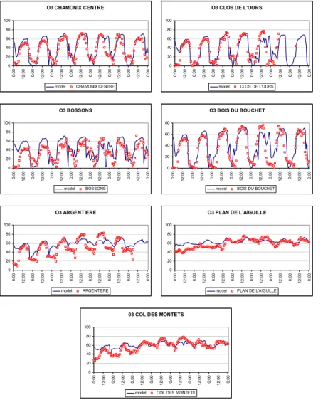
To validate the simulated meteorological fields, we compare the model results to surface observations (Fig. 5). We note that the observed and modelled variables are in good agreement.

5

Temperature at sites ‘Les Houches’, ‘Chamonix’ and ‘Argenti `ere’ shows good am-plitudes for the minimum and maximum, respectively at 01:00 and 13:00 TU. A slight discrepancy at minimal value may be attributed to the difficulties in accurately modelling cooling of lower layer and humidity content of soil canopy at night.

Wind force at site ‘Clos de l’ours’ corresponds to measurement with maximum at

10

13:00 TU, nocturnal cycle is present. The computed wind velocity at the station ‘Bois du Bouchet’ is more important than the real velocity because of a local effect with this station: trees are very close and slow down wind at ground level especially when flowing down valley.

Shifts in wind direction occur at the right times at sites ‘Bois du Bouchet’, ‘Argenti `ere’

15

and ‘Clos de l’ours’ at 08:00 and 20:00 TU.

Profiler data are in good agreement with values from the model (Fig. 6a and b): wind reversal starts and stops at the same time. The altitude of the synoptic wind is well represented. Model results taken into account come from the first layer above the topography. ARPS works with a terrain following coordinate.

20

The boundary layer thickness is well simulated all along the day as it may be ob-served from wind profiler vertical profiles. Discrepancies are obob-served on 9 July, but it is a stormy day with instable weather. More details on dynamics process will be described in a separate paper devoted to dynamics.

Finally, we can say that the simulated meteorological fields are very realistic:

tem-25

perature does not show any bias. The evolution of the thickness of the inversion layer is well simulated. Wind direction and forces are well reproduced with wind reversal observed at the same times in the model and from measurements. Therefore, me-teorological fields may be viewed as realistic enough to drive transport and mixing of

ACPD

Full Screen / Esc

Print Version Interactive Discussion

EGU

chemical species.

5.2. High-resolution chemistry simulation: comparison with surface data

Concentrations of pollutants in the valley (such as O₃ or NO₂) are rather low at least when compared with large cities: values peak at 75 ppb for O₃ and 40 ppb for NO₂ compared to 100 ppb for O₃ and 50 ppb for NO₂ in nearby city of Lyon or Grenoble.

5

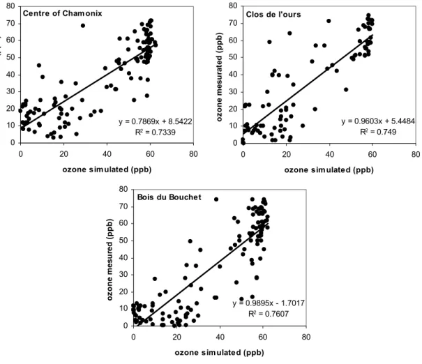
To validate the simulated chemical fields, model results and surface observations are compared during the summer 2003 IPO. Model results taken into account come from the first layer above the topography. TAPOM works with a terrain following coordinate.

Ozone from the observation and from the model is in good agreement in both urban and rural stations (Fig. 7). Both spatial and temporal variability of the simulated ozone

10

concentrations correspond reasonably well to the measured values. Figure 9 shows the correlations between the measured and simulated ozone concentrations for all the IPO days except for the stormy day (9 July 2003). Values of correlation coefficients are significantly high with 0.73<R2<0.76.

These results can be compared to the same correlations in Grenoble during a high

15

ozone episode with R2=0.64 for urban station and R2=0.42 for suburban stations (Couach, 2004).

Background stations (‘Col des Montets’ and ‘Plan de l’aiguille’) are directly under regional influence. The amplitude of the variation of ozone concentrations are low, it does not make sense to give correlation coefficient. The relative mean error on

20

ozone concentration all along the IPO (with the stormy day) is 14% at the site ‘Plan de l’aiguille’ and 6% for the site ‘Col des Montets’ (respectively 12 and 3% without the first day spin up).

It is possible to observe a more important effect of local sources in the south part of the valley: amplitude of ozone concentration is more important for ‘Chamonix centre’,

25

‘Clos de l’ours’, ‘Bossons’ and ‘Bois du Bouchet’. There is a titration of ozone by NO emissions. In the north part of the valley, amplitude of concentration is less important, with values of background at site ‘Argenti `ere’ and ‘Col des Montets’. Road traffic is less

ACPD

Full Screen / Esc

Print Version Interactive Discussion

EGU

important there.

The influence of regional ozone in the valley is preponderant. If we correlate daily maximum of ozone concentration at every site with the concentration of background stations at the same hour, high values of coefficients of correlation are obtained (R2=0.87 for ‘Col des Montets’ station and R2=0.79 for ‘Plan de l’aiguille’ station) as

5

shown with Fig. 10.

Ratio of regional O₃concentration over urban stations daily maximum (at the hour of the maximum) gives important information about regional influence of O₃. High values (≈1) are associated with regional preponderance and lows values with local influence. Here, we have important values (ratio>0.96 when compared with the two background

10

stations).

NO₂ concentration at sites ‘Bossons’, ‘Clos de l’Ours’ and ‘Argenti `eres’ leads to the same conclusion as for ozone (Fig. 8): only the south part of the valley is really affected by traffic emissions. Concentrations of NO₂ decrease when going to the north of the valley. Dilution of pollutants by wind transport is weak: important concentrations are

15

observed only close to the sources. NO₂correlations are satisfactory but an improve-ment of the emission inventory for city and secondary traffic should improve results.

Nitric acid levels are low but well simulated (Fig. 8). CO concentration (Fig. 8) mea-sured and simulated are more than 15 times inferior to the air quality norm (8591 ppb, on 8 h).

20

6. Photochemical indicators to distinguish ozone production regime

Narrow valleys in mountainous environment are very specific areas when it comes to air quality. Emission sources are generally concentrated close to the valley floor, and very often include industries and transport infrastructures. For developing ozone abatement strategies in a specific area, it is important to know whether the ozone production is

25

limited by VOC or NO_x. In order to understand the impact of the emissions sources on ozone production regime, three simulations are performed. All of them are based

ACPD

Full Screen / Esc

Print Version Interactive Discussion

EGU

on meteorology and emission inventory of 7 July 2003. Run B is the simulation of 7 July. Run N corresponds to an arbitrary reduction in NO_x emissions of 50%. Run V is obtained with an arbitrary reduction in VOC emissions of 50%. The three runs are described in Table 5.

7 July 2003, is representative of a summer sunny day with mean pollution level.

5

Photochemical indicators are considered in order to distinguishing NO_x limited and VOC limited ozone formation.

The indicator under consideration is NO_y (NO_y=NO_x+HNO₃+PAN) (Milford et al., 1994). The rationale for NO_yas an indicator is based in part on the impact of stagnant meteorology on NO_x-VOC sensitivity. Stagnant meteorology and associated high NO_x,

10

VOC, and NO_ycause an increase in the photochemical life times of NO_xand VOC, with the result that an aging urban plume remains in the VOC-sensitive regime for a longer period of time. With more vigorous meteorological dispersion and lower NO_x, VOC and NO_yan aging urban plume would rapidly become NO_xsensitive (Milford et al., 1994).

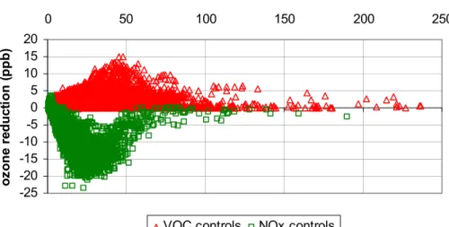
Figure 11 illustrates the NO_x-VOC sensitivity for the simulations (runs N and V) in

15

the bottom of the valley. Only meshes of the terrain with an altitude less than 1500 m above sea level are considered in order to include all the anthropogenic sources. Al-though a significant part of the domain area is rural-type, effects of non rural emission predominate.

The Fig. 11 shows the change in ozone concentrations associated with either

re-20

duced VOC (run V) or reduced NO_x (run N) relative to the domain. The positive val-ues represent locations where, by decreasing the emission, a reduction in ozone is obtained while negative values result from locations where reduced emissions cause more ozone.

According to the results, the ozone production is VOC limited: only a diminution

25

of VOC leads to a reduction of ozone concentration (run V).This conclusion differs from what was observed in the nearby city of Grenoble (100 km from the valley in a Y shape convergence of three deep valleys) where a NO_x controlled regime was observed (Couach, 2004).

ACPD

Full Screen / Esc

Print Version Interactive Discussion

EGU

7. Conclusions

A system of models has been built to model dispersion and evolution of pollutants in a narrow valley. This system is based on several atmosphere dynamics and gas chemistry numerical codes selected for their ability to deal with processes developing at different length and time scales. TAPOM and ARPS codes are used for fine space

5

resolution when CHIMERE and MM5 are used at larger scales.

Three-dimensional photochemical simulations have been performed for a 7 day pe-riod with this system of models, during the POVA intensive pepe-riod of observation in the topographically complex and narrow Chamonix valley. Results from the numerical simulation are in good agreement with observations. Wind direction and forces are well

10

reproduced with wind reversal observed at the same times in the model and from mea-surements. The evolution of the mixed layer thickness induced by thermal convection is well represented with growth in the morning and decay at night. These features of atmosphere dynamics are of major importance for transport and dilution of pollutants.

Computed concentrations are in good agreement with measured values, for both

15

primary and secondary pollutants. Correlation between maximum of ozone and back-ground values (0.8) suggests the regional origin of the pollutant. Dilution of pollutants by wind transport (e.g. NO₂) is weak: important concentrations are observed only close to the sources.

For a later purpose of suggesting reduction strategy, the general trend of chemical

20

process has to be characterized. Well chosen indicators based on some species con-centrations allow to determine a prevailing mechanism. The NO_yindicator shows that the region of the maximum ozone is VOC saturated.

With the transfer of traffic from Chamonix to Maurienne valley because of the acci-dent of Mont-Blanc tunnel, program POVA investigates also Maurienne. As for

Cha-25

monix valley, primary and secondary pollution is considered with measurements and numerical simulations based on the very same system of models. Ozone production regime and indicators obtained in the two valleys will be compared.

ACPD

Full Screen / Esc

Print Version Interactive Discussion

EGU

Acknowledgements. The program POVA is supported by ‘Air de l’Ain et des Pays de Savoie’,

R ´egion Rh ˆone Alpes, ADEME, Primequal 2, METL, MEDD. Meteorological data are provided by M ´et ´eo France and ECMWF, traffic data by STFTR, ATMB, DDE Savoie et Haute Savoie. Computations were done on Mirage. TAPOM comes from the Air and Soil Pollution Laboratory of the Ecole Polytechnique F ´ed ´erale de Lausanne.

5

References

Anquetin, S., Guilbaud, C., and Chollet, J. P.: Thermal valley inversion impact on the dispersion of a passive polluant in a complex mountainous area, Atmos. Environ., 33, 3953–3959, 1999.

Brulfert, G., Chemel, C., and Chollet, J. P.: Numerical simulation of air quality in Chamonix

10

valley, impact of road traffic 16/6–18/6/2003, Avignon, Actes INRETS n◦92, vol. 2, pp. 39– 44, ISSN 769-0266, ISBN 2-85782-588-9, 12th International Scientific Symposium Transport and Air Pollution (INRETS, TUG,NCAR), 2003.

Clappier, A.: A correction method for use in multidimensional time splitting advection algo-rithms: application to two and three dimensional transport, Monthly Weather Revue, 126,

15

232–242, 1998.

Couach, O., Balin, I., Jim ´enez, R., Ristori, R., Kirchner, F., Perego, S., Simeonov, V., Calpini, B., and Van den Bergh, H.: Investigation of the ozone and planetary boundary layer dynamics on the topographically-complex area of Grenoble by measurements and modeling, Atmos. Chem. Phys., 3, 549–562, 2003,SRef-ID: 1680-7324/acp/2003-3-549.

20

Couach, O., Kirchner, F., Jimenez, R., Balin, I., Perego, S., and Van den Bergh, H.: A develop-ment of ozone abatedevelop-ment strategies fort he Grenoble area using modelling and indicators, Atmos. Environ., 38, 1425–1436, 2004.

Espace Mont Blanc: Technical report of the study Air Espace Mont Blanc, 147, Available at: http://www.espace-mont-blanc.com, 2003.

25

Fischer, H., Kormann, R., Kl ¨upfel, T., Gurk, Ch., K ¨onigsted, R., Parchatka, U., M ¨uhle, J., Rhee, T. S., Brenninkmijer, C. A. M., Bonasoni, P., and Stohl, A.: Ozone production and trace gas correlations during the June 2000 MINATROC intensive measurement campaign at Mt. Cimone, Atmos. Chem. Phys., 3, 725–735, 2003,SRef-ID: 1680-7324/acp/2003-3-725. Gong, W. and Cho, H.-R.: A numerical scheme for the integration of the gas phase chemical

ACPD

Full Screen / Esc

Print Version Interactive Discussion

EGU

rate equations in a thre-dimensional atmospheric models, Atmos. Environ., 27A (14), 2147– 2160, 1993.

Grell, G. A., Dudhia, J., and Stauffer, D. R.: A description of the Fifth-Generation Penn State/ NCAR Mesosale Model (MM5), NCAR technical note NCAR/TN-398+STR, NCAR, Boulder, CO., 117, 1995.

5

Grell, G. A., Emeis, S., Stockwell, W. R., Schoenemeyer, T., Forkel, R., Michalakes, J., Knoche, R., and Seidl, W.: Application of a multiscale coupled MM5/chemistry model to the complex terrain of the VOTALP valley campaign, Atmos. Environ., 34 (9), 1435–1453, 2000.

Jimenez, P., Baldasano, J. M., and Dabdub, D.: Comparaison of photochemical mechanisms for air quality modeling, Atmos. Environ., 37, 4179–4194, 2003.

10

Lehning, M., Richner, H., and Kok, G. L.: Pollutant transport over complex terrain: flux and budget calculations fort he POLLUMET field campaign, Atmos. Environ., 30 (17), 3027– 3044, 1996.

L ¨offler-Mang, M., Zimmermann, H., and Fiedler, F.: Analysis of ground based operational net-work data acquired during the September 1992 TRACT campaign, Atmos. Environ., 32 (7),

15

1229–1240, 1998.

Middleton, P., Stockwell, W. R., and Carter, W. P. L.: Aggregation and analysis of volatile organic compound emissions for regional modeling, Atmos. Environ., 241, 5, 1107–1133, 1990. Milford, J. B. and Gao, D.: Total reactive nitrogen (NO_y) as an indicator of the sensitivity of

ozone to reductions in hydrocarbon and NO_x emissions. J. Geophys. Res., 99 (D2), 3533–

20

3542, 2004.

Schmidt, H., Derognat, C., Vautard, R., and Beekmann, M.: A comparison of simulated and observed ozone mixing ratios for the summer of 1998 in Western Europe, Atmos. Envir., 35, 6277–6297, 2001.

Stockwell, R., Kirchner, F., Kuhn, M., and Seefeld, S.: A new mechanism for atmospheric

25

chemistry modelling, J. Geophys. Res., 102 (D22), 25 847–25 879, 1997.

Wotawa, G. and Kromp-Kolb, H.: The research project VOTALP – general objectives and main results, Atmos. Environ., 34 (9), 1319–1322, 2000.

Xue, M., Droegemeir, V., and Wong, V.: The Advanced Regional Prediction System (ARPS) – A multi-scale nonhydrostatic atmospheric simulation and prediction model, Part I: Model

30

dynamics and verification, Meteorology and atmospheric physics, 75, 3/4, 161–193, 2000. Xue, M., Droegemeir, K. K., Wong, V., Shapiro, A., Brewster, K., Carr, F., Weber, D., Liu, Y., and

ACPD

Full Screen / Esc

Print Version Interactive Discussion

EGU

atmospheric simulation and prediction tool, Part II: Model physics and applications, Met. Atm. Phys., 76, 143–165, 2001.

ACPD

Full Screen / Esc

Print Version Interactive Discussion

EGU

Table 1. Hierarchy of computational domains.

Typical extend Grid nodes Grid size Code in use nx E-W×ny N-S ∆x=∆y (km) for simulation

Domain 1 France 1500 km 45×51 27 MM5

Domain 2 Southeastern France 650 km 69×63 9 MM5

Domain 3 Savoie mountains 350 km 96×96 3 MM5

Domain 4 Haute-Savoie Dept. 50 km 67×71 1 ARPS

ACPD

Full Screen / Esc

Print Version Interactive Discussion

EGU

Table 2. Emissions inventory in the area of interest (t.year−1).

CO NMVOC NO_x SO2 PM

Yearly emissions (t.year−1) 827 535 551 194 79

Biogenic sources (% of the year) 0% 51% 2% 0% 0%

Commercial and residential plants (% of the year) 30% 3% 10% 61% 91%

Road transport (% of the year) 70% 19% 88% 39% 9%

Domestic solvent (% of the year) 0% 15% 0% 0% 0%

ACPD

Full Screen / Esc

Print Version Interactive Discussion

EGU

Table 3. Classes of the emission inventory.

Traffic sources Anthropogenic sources Biogenic sources

Heavy vehicles Commercial boiler Forest

Utilitarian vehicles on motorway Residential boiler Grassland Utilitarian vehicles on road Domestic solvent

Cars Gas station

Cars in city Aerial traffic

ACPD

Full Screen / Esc

Print Version Interactive Discussion

EGU

Table 4. IOP meteorology.

05/07/03 06/07/03 07/07/03 08/07/03 09/07/03 10/07/03 11/07/03 Description of the situation Tmin (°C) 4 5 6.5 7 8.5 8 8 Tmax (°C) 22 24 25 26 26 28 27 Isotherm 0°C 3700 m 3850 m 3700 m 4200 m 4000 m 4100 m 4000 m Wind description at 4500 m a.s.l. NW 2.5 m/s NW 4 m/s W 4 m/s (<1m/s) Not significant (<1m/s) Not significant N to NW 5.5 m/s NW 7 m/s 1816

ACPD

Full Screen / Esc

Print Version Interactive Discussion

EGU

Table 5. Runs to determine ozone production regime.

Date Duration Emissions

Run B 7 July 2003 24 h All

Run N 7 July 2003 24 h Run B – 50% NO_x

ACPD

Full Screen / Esc

Print Version Interactive Discussion

EGU

Figure 1. Topography of Chamonix valley: main measurement sites (centre of the valley: Latitude 45.92° N, longitude 6.87° E). Road is the red line.

Fig. 1. Topography of Chamonix valley: main measurement sites (centre of the valley: Latitude

45.92◦N, longitude 6.87◦E). Road is the white line.

ACPD

Full Screen / Esc

Print Version Interactive Discussion EGU

20

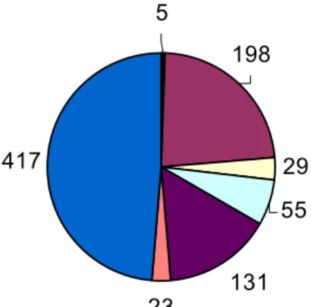
infrastructure coniferous forests broadleaf forests

agricultural domain grassland rock

snow

Figure 2. Landuse of Chamonix valley in summer (km

)

Fig. 2. Landuse of Chamonix valley in summer (km2).

ACPD

Full Screen / Esc

Print Version Interactive Discussion

EGU

21

Figure 3. Geographical description of MM5 (D1, D2, D3) domains over Europe and ARPS (D4,D5) domains over Haute-Savoie department.

Fig. 3. Geographical description of MM5 (D1, D2, D3) domains over Europe and ARPS (D4,D5)

domains over Haute-Savoie department.

ACPD

Full Screen / Esc

Print Version Interactive Discussion

EGU

Figure 4. Description of the modelling system for photochemical simulations. Chemistry solver:

TAPOM Emissions

Dynamic solver: ARPS Meteorology Terrain properties Results of photochemical simulations.

Advanced Regional Prediction System. 300-meter grid cells.

Transport and Air POllution Model.

300-meter grid cells to calculate chemistry. Geographical data from

satellite observations.

Inventory from ‘Air de l’Ain et des Pays de Savoie’. 100-metergrid cells includes land use, population, traffic, industries,..

Chemistry boundary conditions:CHIMERE

Regional ozone prediction model for boundaries of TAPOM.

MM5 forces the field of interest

Fig. 4. Description of the modelling system for photochemical simulations.

ACPD

Full Screen / Esc

Print Version Interactive Discussion

EGU

Figure 5. Meteorological monitoring station compared to results from the simulation.

Fig. 5. Meteorological monitoring station compared to results from the simulation. Measure is

represented by points, model by line.

ACPD

Full Screen / Esc

Print Version Interactive Discussion

EGU

(a)

(b) Fig. 6. (a) Wind force from the wind profiler (left) compared to results (right) from the

compu-tation.(b) Wind direction from the wind profiler (left) compared to results from the computation

(right).

ACPD

Full Screen / Esc

Print Version Interactive Discussion EGU O3 CHAMONIX CENTRE 0 20 40 60 80 100 0: 00 12 :0 0 0: 00 12 :0 0 0: 00 12 :0 0 0: 00 12 :0 0 0: 00 12 :0 0 0: 00 12 :0 0 0: 00 12 :0 0 0: 00

model CHAMONIX CENTRE

O3 CLOS DE L'OURS 0 20 40 60 80 100 0: 00 12 :0 0 0: 00 12 :0 0 0: 00 12 :0 0 0: 00 12 :0 0 0: 00 12 :0 0 0: 00 12 :0 0 0: 00 12 :0 0 0: 00

model CLOS DE L'OURS

O3 BOSSONS 0 20 40 60 80 100 0: 00 12 :0 0 0: 00 12 :0 0 0: 00 12 :0 0 0: 00 12 :0 0 0: 00 12 :0 0 0: 00 12 :0 0 0: 00 12 :0 0 0: 00 model BOSSONS O3 BOIS DU BOUCHET 0 20 40 60 80 0: 00 12 :0 0 0: 00 12 :0 0 0: 00 12 :0 0 0: 00 12 :0 0 0: 00 12 :0 0 0: 00 12 :0 0 0: 00 12 :0 0 0: 00

model BOIS DU BOUCHET

O3 ARGENTIERE 0 20 40 60 80 100 0: 00 12 :0 0 0: 00 12 :0 0 0: 00 12 :0 0 0: 00 12 :0 0 0: 00 12 :0 0 0: 00 12 :0 0 0: 00 12 :0 0 0: 00 model ARGENTIERE O3 PLAN DE L'AIGUILLE 0 20 40 60 80 100 0: 00 12 :0 0 0: 00 12 :0 0 0: 00 12 :0 0 0: 00 12 :0 0 0: 00 12 :0 0 0: 00 12 :0 0 0: 00 12 :0 0 0: 00

model PLAN DE L'AIGUILLE

03 COL DES MONTETS

0 20 40 60 80 100 0: 00 12 :0 0 0: 00 12 :0 0 0: 00 12 :0 0 0: 00 12 :0 0 0: 00 12 :0 0 0: 00 12 :0 0 0: 00 12 :0 0 0: 00

model COL DES MONTETS

Figure 7. O3 monitoring station compared to the model (ppbV); from 05 July 2003 to 11 July

2003, TU, (IOP period).

Fig. 7. O₃monitoring station compared to the model (ppbV); from 5 July 2003 to 11 July 2003,

ACPD

Full Screen / Esc

Print Version Interactive Discussion EGU 27 NO2 BOSSONS 0 20 40 60 80 100 0: 00 12 :0 0 0: 00 12 :0 0 0: 00 12 :0 0 0: 00 12 :0 0 0: 00 12 :0 0 0: 00 12 :0 0 0: 00 12 :0 0 0: 00 model BOSSONS

NO2 CLOS DE L'OURS

0 20 40 60 80 100 0: 00 12 :0 0 0: 00 12 :0 0 0: 00 12 :0 0 0: 00 12 :0 0 0: 00 12 :0 0 0: 00 12 :0 0 0: 00 12 :0 0 0: 00

model CLOS DE L'OURS

NO2 ARGENTIERE 0 10 20 30 40 50 0: 00 12 :0 0 0: 00 12 :0 0 0: 00 12 :0 0 0: 00 12 :0 0 0: 00 12 :0 0 0: 00 12 :0 0 0: 00 12 :0 0 0: 00 model ARGENTIERE CO LES HOUCHES 0 100 200 300 400 500 600 700 800 0: 00 12 :0 0 0: 00 12 :0 0 0: 00 12 :0 0 0: 00 12 :0 0 0: 00 12 :0 0 0: 00 12 :0 0 0: 00 12 :0 0 0: 00 model HOUCHES HNO3 ARGENTIERE 0 2 4 6 8 0: 00 12 :0 0 0: 00 12 :0 0 0: 00 12 :0 0 0: 00 12 :0 0 0: 00 12 :0 0 0: 00 12 :0 0 0: 00 12 :0 0 0: 00 model ARGENTIERE

Figure 8. CO, NO2, HNO3 monitoring station compared to the model (ppbV); from 05 July

2003 to 11 July 2003, TU, (IOP period).

Fig. 8. CO, NO₂, HNO₃monitoring station compared to the model (ppbV); from 5 July 2003 to 11 July 2003, TU, (IOP period).

ACPD

Full Screen / Esc

Print Version Interactive Discussion

EGU

28

Figure 9. Comparison between measured and simulated ozone in three sites for the IPO.

Bois du Bouchet y = 0.9895x - 1.7017 R2 _{= 0.7607} 0 10 20 30 40 50 60 70 80 0 20 40 60 80 ozone simulated (ppb) o zon e m es u re d (ppb) Centre of Chamonix y = 0.7869x + 8.5422 R2 _{= 0.7339} 0 10 20 30 40 50 60 70 80 0 20 40 60 80 ozone simulated (ppb) oz one m es u re d (ppb) Clos de l'ours y = 0.9603x + 5.4484 R2 _{= 0.749} 0 10 20 30 40 50 60 70 80 0 20 40 60 80 ozone simulated (ppb) oz one m es u ra te d (ppb)

28

Figure 9. Comparison between measured and simulated ozone in three sites for the IPO.

Bois du Bouchet y = 0.9895x - 1.7017 R2 _{= 0.7607} 0 10 20 30 40 50 60 70 80 0 20 40 60 80 ozone simulated (ppb) o zon e m es u re d (ppb) Centre of Chamonix y = 0.7869x + 8.5422 R2 _{= 0.7339} 0 10 20 30 40 50 60 70 80 0 20 40 60 80 ozone simulated (ppb) oz one m es u re d (ppb) Clos de l'ours y = 0.9603x + 5.4484 R2 _{= 0.749} 0 10 20 30 40 50 60 70 80 0 20 40 60 80 ozone simulated (ppb) oz one m es u ra te d (ppb)

28

Figure 9. Comparison between measured and simulated ozone in three sites for the IPO.

Bois du Bouchet y = 0.9895x - 1.7017 R2 _{= 0.7607} 0 10 20 30 40 50 60 70 80 0 20 40 60 80 ozone simulated (ppb) o zon e m es u re d (ppb) Centre of Chamonix y = 0.7869x + 8.5422 R2 _{= 0.7339} 0 10 20 30 40 50 60 70 80 0 20 40 60 80 ozone simulated (ppb) oz one m es u re d (ppb) Clos de l'ours y = 0.9603x + 5.4484 R2 _{= 0.749} 0 10 20 30 40 50 60 70 80 0 20 40 60 80 ozone simulated (ppb) oz one m es u ra te d (ppb)

Fig. 9. Comparison between measured and simulated ozone in three sites for the IPO.

ACPD

Full Screen / Esc

Print Version Interactive Discussion

EGU

29

Figure 10. Comparison between daily maximum of O

(6 sites) and concentration of O

at the

same hour for background stations during the IPO.

Regional influence of O3.

Daily max compare w ith 'Col des Montets'

y = 0.8376x + 9.9723 R2 _{= 0.866} 50 55 60 65 70 75 80 50 60 70 80

Daily max of [O3] (ppb)

[O 3] C o l d es M o n tet s ( p p b )

Regional influence of O3.

Daily m ax compare w ith 'Plan de l'aiguille'

y = 0.8577x + 9.7326 R2 _{= 0.7907} 50 55 60 65 70 75 80 50 60 70 80 Daily m ax of [O3] (ppb) [O 3] P lan d e l 'ai g u ill e ( p p b )

29

Figure 10. Comparison between daily maximum of O

(6 sites) and concentration of O

at the

same hour for background stations during the IPO.

Regional influence of O3.

Daily max compare w ith 'Col des Montets'

y = 0.8376x + 9.9723 R2 _{= 0.866} 50 55 60 65 70 75 80 50 60 70 80

Daily max of [O3] (ppb)

[O 3] C o l d es M o n tet s ( p p b )

Regional influence of O3.

Daily m ax compare w ith 'Plan de l'aiguille'

y = 0.8577x + 9.7326 R2 _{= 0.7907} 50 55 60 65 70 75 80 50 60 70 80 Daily m ax of [O3] (ppb) [O 3] P lan d e l 'ai g u ill e ( p p b )

Fig. 10. Comparison between daily maximum of O₃ (6 sites) and concentration of O₃ at the same hour for background stations during the IPO.

ACPD

Full Screen / Esc

Print Version Interactive Discussion EGU 30 NOy -25 -20 -15 -10 -5 0 5 10 15 20 0 50 100 150 200 250 oz o n e r edu ct ion (ppb)

VOC controls NOx controls

Figure 11. NOy according to ozone reduction with NOx and VOC decrease.

Fig. 11. NO_yaccording to ozone reduction with NO_xand VOC decrease.