Static and dynamic data reconciliation for an irrigation canal

HAL Id: hal-00453857

https://hal.archives-ouvertes.fr/hal-00453857

Submitted on 5 Feb 2010

HAL is a multi-disciplinary open access

archive for the deposit and dissemination of sci-entific research documents, whether they are pub-lished or not. The documents may come from teaching and research institutions in France or abroad, or from public or private research centers.

L’archive ouverte pluridisciplinaire HAL, est destinée au dépôt et à la diffusion de documents scientifiques de niveau recherche, publiés ou non, émanant des établissements d’enseignement et de recherche français ou étrangers, des laboratoires publics ou privés.

Malaterre

To cite this version:

Nadia Bedjaoui, Xavier Litrico, Damien Koenig, J. Ribot-Bruno, P.O. Malaterre. Static and dynamic data reconciliation for an irrigation canal. Journal of Irrigation and Drainage Engineering, American Society of Civil Engineers, 2008, 134 (6), pp.778-787. �10.1061/(ASCE)0733-9437(2008)134:6(778)�. �hal-00453857�

Static and Dynamic Data Reconciliation for an Irrigation Canal

N. Bedjaoui∗_{, X. Litrico}†_{, D. Koenig}‡_{, J. Ribot-Bruno}§_{, and P.-O. Malaterre}¶

Abstract

This paper deals with the problem of fault detection and isolation in irrigation canals. We develop a method which combines static and dynamic data reconciliation for the vali-dation of measurements, detection and isolation of sensors and actuator faults and recon-struction of missing data. Static data reconciliation uses static models at a regulation gate to validate measurements and detect sensor and actuator faults. It also enabled us to detect a drift in the stage discharge rating curve. The dynamic data reconciliation uses additional measurements and a dynamic model of the canal in order to validate measurements and detect faults and withdrawals. The combination of the two methods allowed us to distin-guish between withdrawals and faults. Both methods are evaluated on measurements from a real irrigation canal located in the South of France.

1

Introduction

Irrigation represents more than 80% of world fresh water consumption, and most of the irriga-tion systems use open channel to convey water from the resource to the users. The majority of open-channel irrigation canals are managed manually, with large water losses leading to low water efficiency. It is widely accepted that automation can improve water distribution and reduce operational water losses (Plusquellec et al., 1994). But automated systems need to be closely monitored, in order to ensure a proper functioning and detect faults that may affect sensors or actuators.

It may appear simple to detect a fault for a human supervisor. This may be true for a simple system with perfect measurements. In practice however, a measurement is never perfect but always affected by noise. In this case, it is not so easy even for a human supervisor to say whether a measurement is erroneous -presence of faults- or reliable -absence of faults. A solution that is often used e.g. in aeronautics is to equip the system with redundant sensors. Using multiple sensors to measure the same physical variable enables to detect whether one sensors is faulty. This method is very simple (only based on material), but it is however rather expensive, and very few canals are equipped with redundant sensors. This is why it is interesting to develop a method based on analytical redundancy, which uses one sensor for each measured variable, and various models that express physical links between those variables.

∗_{Ph.D., Unit´e Mixte de Recherche Gestion de l’Eau, Acteurs, Usages, Cemagref, B.P. 5095, 34196 Montpellier} Cedex 5, France. e-mail: nadia.bedjaoui@cemagref.fr

†_{Researcher, Unit´e Mixte de Recherche Gestion de l’Eau, Acteurs, Usages, Cemagref, B.P. 5095, 34196} Montpellier Cedex 5, France. e-mail: xavier.litrico@cemagref.fr

‡_{Lecturer, LAG-ESISAR, INPG, France. e-mail: damien.koenig@inpg.fr}

§_{Assistant Engineer, Unit´e Mixte de Recherche Gestion de l’Eau, Acteurs, Usages, Cemagref, B.P. 5095,} 34196 Montpellier Cedex 5, France. e-mail: jose.ribot-bruno@cemagref.fr

The general research line on this subject is called Fault Detection and Isolation (FDI), since the objective is 1) to detect possible faults and 2) to isolate them if possible.

In practice, the main faults that can occur in an irrigation canal are of three kinds:

• actuator fault (e.g. a floating object that tampers the gate), which can be represented

by a bias on the inputs;

• sensor fault (here on the water level measurements), which can be represented by a bias

on the output;

• unmeasured discharge withdrawal occurring at the downstream end of the pool.

There exists different ways to achieve supervision in order to detect and isolate such faults. In Koenig et al. (2005), a bank of unknown input observers is used to detect and isolate actuator faults. In Bedjaoui et al. (2006b), the observers are improved to minimize the H∞ norm of a specified transfer function in order to consider the case of coupled faults. In Deltour et al. (2005), a supervisory monitoring based on data reconciliation is developed for supervision of the Canal de Provence, a large scale system located in the South of France. It is an effective and simple method, which uses a nodal network model of the canal such that each node represents a mass balance equation. The method consists in checking the coherence of daily measurements with this model in order to validate measurements, detect and isolate gross errors and reconstruct missing data. Such a method appears to be very interesting for a manager, but its main drawback is that it neglects the canal dynamics and is not able to detect errors in time.

The main objective of this paper is then to improve this method by developing a generic methodology based on data reconciliation which achieves real-time fault detection and isolation for a supervised irrigation canal. We first perform static data reconciliation at regulation gates in order to detect and isolate sensors and actuators faults. We then use a dynamic model of open-channel flow in order to perform dynamic data reconciliation between two regulation gates. This enables us to detect unmeasured withdrawals.

The proposed method is validated on real data from the Canal de Gignac, an irrigation canal located in the South of France, equipped with a set of sensors, automated gates and a centralized Supervisory Control And Data Acquisition (SCADA) system.

This paper is organized as follows: the problem statement and describes the developed method-ology. Section 3 explains data reconciliation principle in the static and dynamic cases. Section 4 illustrates the main results of the methodology on real data from Gignac canal.

2

Problem Statement

An irrigation canal can be represented as a series of pools separated by regulation gates. In most canals, measurement devices such as water level sensors, gate position sensors and in some cases velocity sensors are available close to the regulation gates. Fig. 1 represents a canal with gates, and water level sensors hi, gate position sensors ui and a velocity sensor v.

We consider in this paper three kinds of faults that can occur in irrigation canals:

• actuator fault (e.g. a floating object that tampers the gate), which can affect the gate

position ui;

• sensor fault which can affect the water level measurements hior the velocity measurement

6 u3 y3 y₁ 6 6 u2 u1 ® p1 ® p₂ y2 y0 y4 -v . . . .. . . . . . . . . . . . . ..._.. .. .. .. .. .. .. .. .. .. .. . . . . . . . . . . . . ... .. .. .. .. .. .. .. .. .. .. . . . . . . .. .. .. .. .. .. .. .. .. .. . Local approach Local approach Local approach .. .. .. .. .. .. .. .. .. .. .. . Global approach Global approach . . . . . . . . . . . . . .. .. .. .. .. .. .. .. .. .. .. .. . . . . . .. .. .. .. .. .. .. .. .. .. .. .. . . . . . . . .

Figure 1: Schematic view of a canal with two pools

• unmeasured discharge withdrawal occurring along the pool. The total withdrawal

dis-charge can be represented at the downstream end of the pool represented as pi.

It should be noted that locally, an actuator or a sensor fault has the same effect on the flow discharge that has a withdrawal. Indeed, a floating object that tampers the gate u2 reduces

the gate opening section leading to a gate flow discharge lower than what it should be. This has locally the same effect as a withdrawal. In the same way, a bias occurring for example on a water level sensor h1 will affect the discharge estimation given by the gate equation. If this

fault is not detected, the manager may want to correct the discharge by adjusting the gate opening. This will have an effect on the water distribution, in the same way as a unpredicted variation of discharge withdrawal.

It is therefore of utmost importance for the manager to be able to detect such faults, if possible as soon as they occur and be able to distinguish between them (to say if it is a withdrawal, a sensor fault or an actuator fault) which is not easy in practice. When analyzing the problem, we found that: locally (at regulation gates), one can only detect sensor or actuator faults but not withdrawals, since they don’t affect the discharge flowing through the gate; globally (on the whole pool), one can detect faults or withdrawals but can not isolate them and; by combining both local and global analysis, one may distinguish withdrawals from sensor or actuator faults. The methodology developed in this paper is then based on the combination of two approaches as follows:

1. Local approach: where static data reconciliation based on analytical redundancy and local measurements is applied at regulation gates in order to detect and isolate sensor and actuator faults;

2. Global approach: where dynamic data reconciliation based on linearized Saint-Venant equations of the pool is applied to the whole pool in order to detect withdrawals and faults;

3. Combination of local and global approaches: in order to isolate withdrawals from sensor and actuator faults.

In order to show the efficiency of the developed methodology, we give the main obtained results of its application on real data of the Canal de Gignac. But let us first present the principle of data reconciliation method in static and dynamic cases.

3

Data Reconciliation

Roughly speaking, data reconciliation generates, from given measurements, a set of data in coherence with the process model. The obtained data are then compared to the measurements to generate residuals. These residuals are checked using statistical tests, which may or not detect the presence of fault.

3.1 General Framework for Data Reconciliation

Data reconciliation requires a process model and the statistical characteristics of the measure-ments. The model is the set of physical relations between the system variables denoted x1, .., xn. When these variables can be evaluated by sensors, they correspond to the measurements and are denoted y_m1, ..., y_mn. A subscript index k is also used to denote the value of the variable at time k∆t, where ∆t is the sampling period of measurement.

When the model is static, the variables are linked by a static relationship of the following form:

M Yk= R (1)

where Yk = £

y1k ... ynk ¤_T

is the measurement vector, M and R are respectively a matrix and a vector of appropriate dimensions.

When the model is dynamic, the system variables are linked by a dynamic relationship of the following form: X_k+1 = AX_k Yk = CXk (2) where Xk = £ x1k ... xnk ¤_T

and Xk+1 are the vector representations of the set of system variables respectively at time k∆t and (k + 1)∆t and A is a matrix of appropriate dimension. We model a sensor by an additive noise. Then, sensor i delivers a measurement y_mi of variable

yi such that:

ymi = yi+ ²i

This noise ²i is assumed to follows a Gaussian probability density function N with zero mean and a standard deviation σ_i.

Hence, the measurements vector Ym is affected by the Gaussian noise vector ² = (²1, ..., ²n)T with zero mean and variance-covariance matrix V.

Ym = Y + ² ² ∼ N (0, V)

As the sensors are assumed to be independent, the variance-covariance matrix V is diagonal:

V = diag(σ2₁, · · · , σ_n2)

3.2 Static Data Reconciliation

3.2.1 Principle

Static reconciliation consists in obtaining estimated values ˆY close to the measurements Ymand which satisfy the static linear model (1). This can be formulated as an optimization problem with static constraints. The performance index to minimize is the quadratic error between the measurements Ym and the reconciled data ˆY . The constraints are given by the model (1).

Mathematically, it reads: _   min_Yˆ 1₂ ° ° °Ym− ˆY ° ° °2 V−1 M ˆY = R (3) The solution is given by (Wang et al., 2004):

ˆ

Y = (In− SM )Ym+ SR (4) where S = VMT_{(M VM}T₎−1 _{and I}

n∈ Rn×n is the identity matrix.

This solution can easily be implemented in any computer language, in order to generate esti-mates ˆY that satisfy the model (1).

A second step is to check the consistency of the measurements. This is done with statistical tests.

3.2.2 Statistical tests

Statistical tests are used to check the consistency of the measurements. In practice, a threshold is needed to decide whenever an error is detected. This threshold is generally fixed for a given confidence level and for a given probability distribution. The following statistical tests are classically used to detect and localize the possible errors:

• Global Test: It allows us to check the global coherence of measurements with the model

(Bagajewicz, 2000). It uses the global residual r_G defined by:

rG = M Ym− R

In the absence of faults, this residual has the following properties:

E(rG) = 0 and Vr = Var(rG) = M VMT

where E(r_G) stands for the mean of r_G and Var(r_G) represents its variance and the quantity φ = r_GTV_r−1rGfollows a χ2 probability density function of nddegrees of freedom, where nd = n − nr, with n the number of measurements and nr the number of global residuals (Bagajewicz, 2000):

φ ∼ χ2(nd)

The threshold is determined in the χ2 table for a confidence level of 95% (for example). The test consists then in evaluating whether the variable φ remains lower than the thresh-old. This global test allows only fault detection. It can not give more information (the number of erroneous measurement(s), the origin of the fault(s)). It is why, the nodal test is usually used.

• Nodal Test: When there is no error, each normalized global residual element ri = √rGi_V ri follows the centralized reduced Gaussian probability density function (Bagajewicz, 2000):

ri∼ N (0, 1), ∀i = 1, nr

As for the global test, we fix a threshold. For a reduced centered probability density function and for 95% of confidence level, the threshold is ±1.96. The nodal test then consists in checking if

|ri| < 1.96

In the presence of fault(s), only the affected residuals cross the threshold. Consequently, this test suspects only the variables xi that compose these residuals and especially the common variables which can give an idea of the origin of the fault.

3.3 Dynamic Data Reconciliation

3.3.1 Principle

In the control field, data reconciliation is a part of the general problem of state estimation in the dynamic systems. Generally, it is solved by the Kalman filter. Dynamic data reconciliation is based on a dynamic model of the form:

Xk+1 = AXk

Yk = CXk (5)

where X ∈ Rn is the state vector, Y ∈ Rm is the measurement vector, A ∈ Rn×n is the state matrix and C ∈ Rm×n _{is the observation matrix.}

Data reconciliation is solved by the Kalman filter (Dibo, 2005). The Kalman filter is a recursive method which computes state estimation and state variances (Benqlilou, 2004). It uses the model (5) and supposes that the measurement vector Ym is affected by a white noise vector ² such that (Welch and Bishop, 2004).

Ym = Y + ²

² ∼ N (0, V), E(²i²j) = 0, j 6= i, i, j = 1, n The Kalman filter is of the form:

ˆ

Xk+1 = A ˆXk+ K(Yk− ˆYk) ˆ

Y_k= C ˆX_k (6)

where ˆX_kis the state estimate of X_k. K is the filter gain determined by minimizing the variance Γk of the estimation error ek (Welch and Bishop, 2004):

ek= Xk− ˆXk (7)

min

ˆ

X

{Γ_k= E[e_keT_k]} (8)

The filter gain K is then obtained by:

K = ΓCT(CΓCT + Vy)−1 where Γ is the stationary solution of a Riccati equation.

3.3.2 Statistical test for the error estimation

The statistical test is used to check if the quantity eyk is normal:

eyn ∼ N (0, 1) where eyn = eyk/

q

Ve_yk is the normalized output estimation error, eyk = Yk− ˆYk the output estimation error and Ve_yk is its variance.

In this case, for a confidence level of 95% the threshold is ±1.96.

In this section, we have given a summary of the data reconciliation method in the static and dynamic cases. In the next section, we will show its application to irrigation canals.

4

Application to the Canal de Gignac

The canal de Gignac is a real site which allows testing new modeling and control methods. It includes 5 stations among them the Belbezet and the Partiteur stations equipped with measurement and automatic control devices. At the Partiteur station, the canal is divided into two branches, the right bank (RB) and the left bank (LB). In each branch, we find an automatic regulation gate, two water level sensors and a velocity sensor. The canal supervisor displays data and saves them into a database.

In this paper, we are interested in validating measurements of the pool situated between Bel-bezet and Partiteur Right Bank. To this end, we proceed as follows:

1. We apply data reconciliation locally at the Partiteur Right Bank regulation gate. 2. We use Kalman filtering for the whole pool Belbezet-Partiteur Right Bank. Let us first describe the available models and measurements.

4.1 Description of the available sensors

The following sensors are available at the regulation gate:

• Position gate sensor: The regulation gate (see fig. 2) is submerged. It is equipped with

a motor which acts on the gate according to the automate consigns. The gate is also equipped with a position sensor.

• Water level sensors: The water level sensors are piezo-resistive sensors, whose resistance

varies with the water level.

• Velocity sensor: The velocity sensor is an ultrasonic sensor, which measures the average

water velocity based on the transit time ∆T of an ultrasonic signal between points A and B in Fig. 3. The velocity is obtained with the following formula:

V = L 2cosα( 1 TAB − 1 TBA )

where L is the length AB, α is the angle with respect to the flow direction, T_AB is the propagation time from A to B and TBA is the propagation time from B to A.

Figure 2: Partiteur Right Bank regulation gate A B V α cos V α α C C L D a b c C Ultrasonic sensor Right bank Left bank A B V α cos V α α C C L D a b c C Ultrasonic sensor A B V α cos V α α C C L D a b c C Ultrasonic sensor Right bank Left bank

Figure 3: Principle of the velocity sensor

A measure is usually given with an absolute or relative uncertainty. This uncertainty indicates the error of the sensor. This error can be deterministic represented by the systematic uncer-tainty, or stochastic due to the measurement noise. To compute the measurement variance, we use the fact that for a confidence level of 95%, the uncertainty is twice the standard deviation (Ragot et al., 1990):

σ2 = (1 2∆)

2

The measurements variances are then given by σh = 7 × 10−3m, σu = 5 × 10−3m, σv = 3 × 10−2_m/s.

4.2 Description of Nonlinear available Models of Flow Discharge

There is no flow discharge sensor. The flow discharge is computed using models. We use three static flow discharge models:

• The gate equation:

Qv = CdLU2

p

where Cd is the discharge coefficient, L the gate width and g the gravity acceleration. U2

represents the gate opening, H₁ and H₂ the upstream and downstream water levels of the gate and Qv is the flow discharge. For the considered gate the parameters are given by Cd= 0.68 and L = 1.53m.

• The stage discharge rating curve: The stage discharge rating curve relates the discharge Q to the downstream water elevation H2. The stage discharge rating curve is given by:

Qct = a(H2− H0)b (10)

Where a, b are constants and H0 is the water level for which the flow discharge is null, H2 represents the downstream water level of the gate and Qct the flow discharge. In our case, we have a = 1.95 × 10(−4+2b)_{, b = 1.8126 and H}

0= 1.4 × 10−2m.

• The velocity model: The velocity model allows us, according to the straight line velocity V_L (given by the velocity sensor) and the water level H to determine the flow discharge

Q by the equation:

Qcv= LcVLH(c1+ c2H + c3H2) (11)

Where Lc is the canal width, c1, c2 and c3 are coefficients determined experimentally

(L_c= 1.33m, c₁ = 1.8445, c₂ = −1.9594 and c₃ = 0.9383).

4.3 Linearized Models for Data Reconciliation

The previous models are nonlinear. In order to apply data reconciliation based on linear models, we linearize them around the operating point. This leads to:

• Gate equation:

q2 = k1h1+ k2h2+ kuu2 (12)

where k1, k2and kuare constants, obtained by differentiating Eq. (9) with respect to H1, H2and U2, respectively. h1, h2, u2 and q2represent the upstream water and downstream

water level variations, the gate opening variation and the discharge variation around the operating point, respectively.

• Stage discharge rating curve:

q2 = kcth2 (13)

with kct a constant obtained by differentiating Eq. (10). h2 and q2 are the downstream

water level and the discharge variations around the operating point.

• Velocity model:

q2 = khh2+ kvv (14) where k_h and kv are constants obtained by differentiating Eq. (11). h2 and v represent

4.4 Local Approach: Application of Static Data Reconciliation

We now apply data reconciliation based on the three linearized models. A first reconciliation is performed to check whether the measurements are coherent with the model. Then, a bias is artificially added on the gate opening, to test whether the method can detect this bias. Finally, we show that our method also enables to detect a slow drift in one of the models.

We apply data reconciliation during 9 days (from April 16th to April 24th). The variables used in the data reconciliation are as follows. The state vector is given by Y = [h1 h2 u2 v q2]T, the

measurement vector by Ym= [h1m h2m um vm] and the discharge q2 is not measured. Assuming that the sensors are independent, the variance-covariance matrix of Y is given by:

V = diag(σ2_h1, σ2_h2, σ2_u2, σ2_v)

Three models are available to compute the discharge q2: the gate model (12), the rating curve

model (13) and the velocity model (14). After elimination of the unmeasured discharge q2, we

obtain a model of the form M Y = R where R = 0,

M =

µ

k1 k2− kct ku 0

0 ky− kct 0 kv

¶

and consequently a global residual vector r_G = M Y_m− R of two elements r_1G and r_2G given by:

r1G = M1Ym− R1, with M1 = ( k1 k2− kct ku 0 ) and R1= 0 and

r_2G = M₂Y_m− R₂, with M₂= ( 0 k_h− k_ct 0 k_v ) and R₂ = 0

Before showing the test results, let us study the possible fault cases: The residual r1 uses h1, h2 and u2 while the residual r2 uses only h2 and v. In this case, we can have the three different

situations:

• Only r1 crosses the threshold: there exists an error on the upstream water level h1 or the

gate position measurement u2.

• Only r2 crosses the threshold: there exists an error on the velocity measurement. • Both r1 and r2crosses the threshold: there exists an error on the downstream water level

measurement h2.

This can be summarized in Table 1.

r1 = 0 r1 = 1 r2 = 0 ® h1∪ u2 r₂ = 1 v h₂

Table 1: Decision table Let us now show the tests results.

4.5 Data reconciliation results without bias

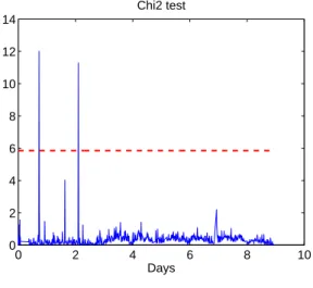
4.5.1 Global test The residual is given by:

φ = r_GTV_r−1r_G ∼ χ2(2)

In this case, the threshold corresponding to a χ2 _{probability density function of 2 degrees of}

freedom and for a confidence level of 95% (α = 0.05 in the χ2 _{table) is 5.85:}

If φ > 5.85, then there is detection of a fault

0 2 4 6 8 10 0 2 4 6 8 10 12 14 Chi2 test Days

Figure 4: Global test

The quantity φ is evaluated for a 9 days period (see Fig. 4). Except some punctual detections, the values of φ are always under the threshold which means that there is no fault. As the mea-surements are emitted to the supervisor through a network radio and phone transmission and saved in a database, the punctual detections may be due to a radio transmission interruption, absence of data in the database or other external phenomena independent of sensors.

As the global test validates the measurements, it is not necessary here to apply the nodal test. However, we show it here for a simple illustration.

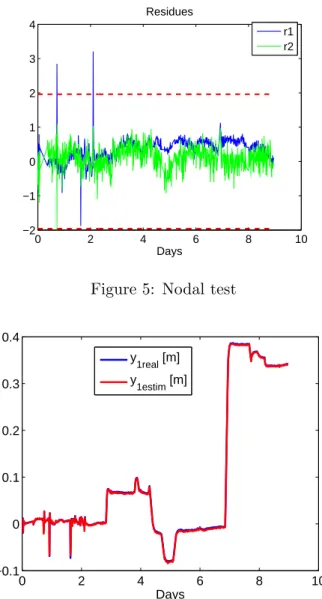
4.5.2 Nodal test

The nodal test is used to check that each normalized element of the global residual vector remains under the threshold:

If |r1| > 1.96 or |r2| > 1.96 then there is detection of a fault

The figure 5 shows that except punctual detection due to previous explanation, the residuals do not cross the threshold. Consequently, there is no detection of any fault.

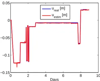
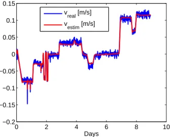
4.5.3 Data Reconciliation:

Finally, one may reconcile the data with the models using static data reconciliation. The figures 6-9 illustrate the original and reconciled measurements.

The graphs show that the reconciled values are close to the measurements values.

0 2 4 6 8 10 −2 −1 0 1 2 3 4 Residues Days r1 r2

Figure 5: Nodal test

0 2 4 6 8 10 −0.1 0 0.1 0.2 0.3 0.4 Days y_1real [m] y 1estim [m]

Figure 6: Upstream water level variation

4.5.4 Data reconstruction:

The figure 10 draws the estimated discharge. Data reconciliation has therefore been performed successfully to validate the measurements on a regulation gate of the Canal de Gignac. Let us now evaluate the ability of the method to detect a bias.

4.6 Data reconciliation results with a bias

In order to simulate faults, we have added during a period of time a 5 cm bias on the position gate. The same procedure is applied as in the no fault case.

4.6.1 Global test

In the global test, the residual crosses the threshold when the fault occurs (see figure (11)). The global test therefore correctly detects the presence of a fault but it can not isolate it, since we cannot determine which measurement is affected.

0 2 4 6 8 10 −0.2 −0.1 0 0.1 0.2 0.3 Days y_2real [m] y 2estim [m]

Figure 7: Downstream water level variation

0 2 4 6 8 10 −0.15 −0.1 −0.05 0 0.05 Days u real [m] u_estim [m]

Figure 8: Gate Position variation

4.6.2 Nodal test

Using the nodal test, we see that a bias is detected only on the residual r1 (see Fig. 12).

According to the table decision (table 1), one can suspect that the fault is on u2 or h1. But

there is no more information that deduces that the fault is on u2. Consequently, we have partial

isolation only.

4.7 Stage discharge rating curve drift

An interesting output of this method is that it may also detect slow drifts in the models. Indeed, when we consider data reconciliation on a longer time period (90 days), we have obtained the results depicted in Fig. 13 for the individual residuals.

0 2 4 6 8 10 −0.2 −0.15 −0.1 −0.05 0 0.05 0.1 0.15 Days v_real [m/s] v estim [m/s]

Figure 9: Velocity variation

0 2 4 6 8 10 −0.5 −0.4 −0.3 −0.2 −0.1 0 0.1 0.2 Days q_estim [m3/s]

Figure 10: Estimated discharge variation

table (table 1), one can conclude that the sensor h2 is faulty. But it wasn’t the case. It was a

model drift and especially it was the rating curve model drift. This can be explained by the fact that this model is not time invariant, but time varying, since the friction changes with time: there are weeds that grow inside the canal, and that progressively change its friction. The proposed method can therefore detect a model drift, in this specific case due to a change in the friction coefficient due to weeds growing in the canal.

A possible way to overcome this model drift is to adapt the model for different periods of year (spring, summer, autumn). In this case, one may use a set of linear models to represent the system. Such developments are out of the scope of the present paper and will be considered in the perspectives.

0 2 4 6 8 10 0 5 10 15 Chi2 test Days

Figure 11: Global test

0 2 4 6 8 10 −3 −2 −1 0 1 2 3 4 Residues Days r1 r2

Figure 12: Detection only on the first residual

4.8 Global Approach: Application of Dynamic Data Reconciliation

We now apply the dynamic reconciliation method to a pool of the Canal de Gignac. The considered system is the pool Belbezet-Partiteur, which is a 4.3 km long pool, with average slope 0.0004 and a general rectangular cross section, of width 2.5 m. To simplify the study, we consider the system represented in figure 14 where:

• q1 is the Belbezet discharge variation.

• h1 is the upstream water level variation of the Partiteur regulation gate. • h2 is the downstream water level variation of the Partiteur regulation gate. • u₂ is the Partiteur regulation gate position variation.

• p1 is the offtake discharge variation.

10 20 30 40 50 60 70 80 90 100 −8 −6 −4 −2 0 2 4 6 8 Residues Days r1 r2

Figure 13: Individual residuals r1 and r2

q1 u2 y1 -6 -ª p1 6 y2 q2 _-v

Figure 14: Schematic representation of one canal-pool

noises ²_h1, ²_h2, ²_u2 and ²_v with zero mean and respective variances V_h1, V_h2, V_u2 and V_v. The discharge p1 is not measured. The discharge q1 is not measured but assumed to be reconciled

locally by data reconciliation at the Belbezet regulation gate. This step is not detailed here, but is very similar to the static reconciliation exposed earlier in the paper. We therefore use the discharge q1 as a measurement affected by a white noise ²q1 with zero mean and variance

Vq1. The variance-covariance matrix then reads:

V = diag(Vq1, Vu2, Vh1, Vh2) 4.9 Dynamic modeling of the canal pool

In order to apply dynamic data reconciliation, the canal pool is represented by its dynamic model derived from the rational linearized Saint-Venant equations (15) coupled with the lin-earized gate equation (16).

h1(s) = p21(s)q1(s) + p22(s)(q2(s) + p1(s)) (15)

Where p21and p22represent low frequency approximations of the pool transfer functions defined

in (Litrico and Fromion, 2004).

q₂(s) = k₁h₁(s) + k₂h₂(s) + k_uu₂(s) (16)

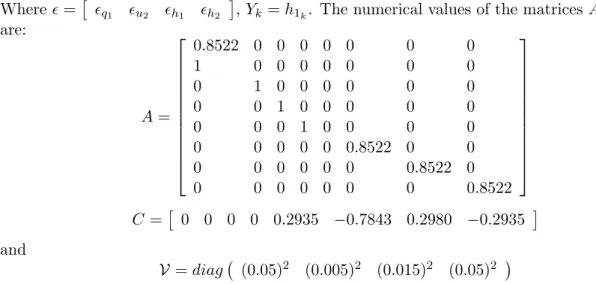
The canal dynamic model is obtained from the combination of the rational linearized Saint-Venant equations (15) and the linearized gate equation (16). The resulting model is of the form:

Xk+1 = AXk

Where ² =£ ²q1 ²u2 ²h1 ²h2

¤

, Yk= h1k. The numerical values of the matrices A, C and V are: A =             0.8522 0 0 0 0 0 0 0 1 0 0 0 0 0 0 0 0 1 0 0 0 0 0 0 0 0 1 0 0 0 0 0 0 0 0 1 0 0 0 0 0 0 0 0 0 0.8522 0 0 0 0 0 0 0 0 0.8522 0 0 0 0 0 0 0 0 0.8522             C =£ 0 0 0 0 0.2935 −0.7843 0.2980 −0.2935 ¤ and V = diag¡ (0.05)2 _(0.005)2 _(0.015)2 _(0.05)2 ¢

Based on this model, we reconcile the measurements using the Kalman Filter (6). Then, we check the well reconciliation of the measurements through the error estimation test.

4.10 Dynamic data reconciliation results

The database is taken as in the static case (from the April 16th to April 23th, 2006) and the results are illustrated in figure 15. We can clearly observe that there is a fault detection from the middle of the second day. Otherwise, we can say that there is no fault. The eventual faults can be on h₁, h₂, v, u₂ or p₁. To have more information on the fault origin, we look to the local data reconciliation results illustrated for the same period in figure 5.

0 1 2 3 4 5 6 7 8 −20 −15 −10 −5 0 5 Days

Normalized Estimation error e

y

n

e

y n

Figure 15: Normalized estimation error ehn = (Yk− ˆYk)/

√ Veh

4.11 Combination (Local/Global) approaches

We use a combination of static and dynamic data reconciliation. The static data reconciliation based on the three quoted models and the dynamic data reconciliation based on the dynamic model of the pool coupled to the gate equation.

To summarize all the results, we can say that:

1. The local approach based on static data reconciliation can:

• Validate measurements

• Detect actuator and sensor faults only • Detect drift model

• Isolate partially or (totally in some cases) the faults

2. The global approach based on dynamic data reconciliation can:

• Validate the measurements

• Detect actuator, sensor and system faults (withdrawals)

3. The combination of the two approaches can distinguish the withdrawals from the other faults.

5

Conclusion

This paper deals with sensor and actuator fault detection and isolation in irrigation canals using data reconciliation. We have first presented the problem statement and showed how we proceeded to develop a generic methodology for canals which are equipped with regulation and then, we presented the data reconciliation method in the static and dynamic cases. After that, we showed the main results obtained from its application to real data from the Canal de Gignac.

The results showed that static data reconciliation based on the three discharge models which are the discharge rating curve model, the gate equation and the velocity model, enables to validate the measurements, to detect faults, to isolate partially or totally them. It also enables us to reconstruct the discharge, which is not measured and detect the stage discharge rating curve model drift. This drift is due to the grow of weeds affecting consequently the canal roughness. Dynamic data reconciliation based on Kalman Filtering on the Belbezet-Partiteur pool of the Canal de Gignac uses a dynamic model derived from the linearized Saint-Venant model coupled with the linearized gate equation. We have shown that the method allows to detect either withdrawals or faults but can not isolate them. By combining the dynamic (global approach) and the static (local approach) data reconciliation, we showed that we are able to distinguish between them.

Such a method can be generalized to help the manager of open-channel systems, in order to detect possible faults occurring on the system.

6

Acknowledgement

The writers acknowledge the financial support of R´egion Languedoc-Roussillon, Conseil G´en´eral de l’H´erault, Agence de l’Eau Rhˆone-M´editerran´ee-Corse and Cemagref through the “Plate-forme Exp´erimentale du Canal de Gignac.”

7

Notations

The following symbols are used in this paper: ˆ= notation for estimated values;

Q = steady state discharge in m3_s−1_;

q = discharge deviation in m3s−1;

t = time in s;

U = absolute gate opening in m; u = gate opening deviation in m; X = state vector;

xi = ith state variable;

Ym = vector of measurements;

ymi = ith measurement;

hi = ith water level measurement;

References

M.J. Bagajewicz (2000). A brief review of recent developments in data reconciliation and gross error detection /estimation, Latin American Research, Vol 30, pp 335-342.

N. Bedjaoui, X. Litrico, A. Lourosa, J.R. Bruno, (2006). Application of data reconciliation on an irrigation canal. in 7th conference on Hydroinformatics, vol. II, pp. 1503-1510, Nice. N. Bedjaoui, X. Litrico, D. Koenig and P.-O. Malaterre, (2006). H∞ observer design for

time-delay systems. Application to FDI for irrigation canals, in The 45th IEEE Conference on

Decision and Control, San Diego, USA.

C. Benqlilou, (2004). Data reconciliation as framework for chemical processes optimization and control. Ph.D. thesis, Universitat Politecnica de Catalunya.

J.-L. Deltour, E. Canivet, F. Sanfilippo and J. Sau (2005). Data reconciliation on the complex hydraulic system of Canal de Provence. J. Irrig. Drain. Eng., 131(3):291–297.

M.A. Dibo, (2005). Validation de donn´ees et diagnostic des syst`emes incertains `a l’aide de l’analyse par intervalle. Ph. D. thesis INP Lorraine.

D. Koenig, N. Bedjaoui, and X. Litrico, (2005) Unknown Input Observer for time-delay systems: Application to FDI for irrigation canals, in 44th IEEE Conference on Decision and Control, pp. 5794-5799, Seville, Spain.

X. Litrico, and V. Fromion, (2004), Analytical approximation of open-channel flow for controller design, App. Math. Mod, Vol 28, pp. 677-695

H. Plusquellec, C. Burt and H.W. Wolter, (1994), Modern Water Control in Irrigation, The World Bank, Irrigation and Drainage Series, n. 246.

J. Ragot, D. Maquin, M. Darouach and G. Bloch, (1990), Validation de donn´ees par ´equilibrage de bilan. Trait´e des nouvelles technologies, s´erie diagnostic et maintenance, Herm`es, 1990. . J. Ragot and D. Maquin, (2005). Validation et r´econciliation de donn´ees. Approche

conven-F. Wang, X.P. Jia, S.Q. Zheng, J.C. Yue, (2004). Improved NT-MT method for gross error detection and data reconciliation, Computers and Chemical Engineering, Vol 24, pp2189-2192.

G. Welch and G. Bishop, (2004) An introduction to the Kalman Filter, Technical report TR

95-041, Department of Computer Science, University of North Carolina at Chapel Hill.

S. Choy, E. Weyer, (2005) Reconfiguration schemes to mitigate faults in automated irrigation channels, in 44th IEEE Conference on Decision and Control, pp. 1875-1880, Seville, Spain. Y. Yang, R. Ten and L. Jao, (1995), A study of gross error detection and data reconciliation