Application of a high-resolution weather model in the area of the western Gulf of Corinth for the tropospheric correction of interferometric synthetic aperture radar (InSAR) observations

(1)

HAL Id: tel-02967065

https://tel.archives-ouvertes.fr/tel-02967065

Submitted on 14 Oct 2020

HAL is a multi-disciplinary open access

archive for the deposit and dissemination of sci-entific research documents, whether they are pub-lished or not. The documents may come from teaching and research institutions in France or abroad, or from public or private research centers.

L’archive ouverte pluridisciplinaire HAL, est destinée au dépôt et à la diffusion de documents scientifiques de niveau recherche, publiés ou non, émanant des établissements d’enseignement et de recherche français ou étrangers, des laboratoires publics ou privés.

Application of a high-resolution weather model in the

area of the western Gulf of Corinth for the tropospheric

correction of interferometric synthetic aperture radar

(InSAR) observations

Nikolaos Roukounakis

To cite this version:

Nikolaos Roukounakis. Application of a high-resolution weather model in the area of the western Gulf of Corinth for the tropospheric correction of interferometric synthetic aperture radar (InSAR) observations. Ocean, Atmosphere. Université Paris sciences et lettres; Panepistīmio Patrṓn, 2019. English. �NNT : 2019PSLEE042�. �tel-02967065�

(2)

Préparée à l’Ecole Normale Supérieure

Dans le cadre d’une cotutelle avec Université de Patras, Grèce

Application d'un modèle météorologique à haute résolution à la

correction troposphérique d'observations interférométriques de

radar à synthèse d'ouverture (InSAR) dans la région de l'ouest

du golfe de Corinthe, Grèce

Application of a high-resolution weather model in the area of the

western Gulf of Corinth for the tropospheric correction of

interferometric synthetic aperture radar (InSAR) observations

Soutenue par

Nikolaos ROUKOUNAKIS

Le 23 Octobre 2019

Ecole doctorale n° 560

Sciences de la terre et de

l’environnement et physique

de l’univers, Paris

Composition du jury :

Stéphane, JACQUEMOUD

Université Denis Diderot – Paris VII Président

Konstantinos, KATSAMPALOS

Université Aristotle de Thessaloniki Rapporteur

Laurent, MOREL

CNAM, Le Mans Rapporteur

Cécile, DOUBRE

Ecole et Observatoire des Sciences de la Terre, Strasbourg Examinateur

François, LOTT

CNRS, Paris Examinateur

Athanassios, ARGIRIOU

Université de Patras Directeur de thèse

Pierre, BRIOLE

(3)

(4)

ii

Abstract

Space geodesy techniques (SAR interferometry and GNSS) have recently emerged as an important tool for mapping regional surface deformations due to tectonic movements. A limiting factor to this technique is the effect of the troposphere, as horizontal and vertical surface velocities are of the order of a few mm yr-1, and high accuracy (to mm level) is essential. The troposphere introduces a path delay in the microwave signal, which, in the case of GNSS Precise Point Positioning (PPP), can nowadays be successfully removed with the use of specialized mapping functions. Moreover, tropospheric stratification and short wavelength spatial turbulences produce an additive noise to the low amplitude ground deformations calculated by the (multitemporal) InSAR methodology. InSAR atmospheric phase delay corrections are much more challenging, as opposed to GNSS PPP, due to the single pass geometry and the gridded nature of the acquired data. Several methods have been proposed, including Global Navigation Satellite System (GNSS) zenithal delay estimations, satellite multispectral imagery analysis, and empirical phase/topography estimations. These methods have their limitations, as they rely either on local data assimilation, which is rarely available, or on empirical estimations which are difficult in situations where deformation and topography are correlated. Thus, the precise knowledge of the tropospheric parameters along the propagation medium is extremely useful for the estimation and minimization of atmospheric phase delay, so that the remaining signal represents the deformation mostly due to tectonic or other geophysical processes.

In this context, the current PhD Thesis aims to investigate the extent to which a high-resolution weather model, such as WRF, can produce detailed tropospheric delay maps of the required accuracy, by coupling its output (in terms of Zenith Total Delay or ZTD) with the vertical delay component in GNSS measurements. The model initially is operated with varying parameterization in order to demonstrate the best possible configuration for our study, with GNSS measurements providing a benchmark of real atmospheric conditions. In the next phase, the two datasets (predicted and observed) are compared and statistically evaluated for a period of one year, in order to investigate the extent to which meteorological parameters that affect ZTD, can be simulated accurately by the model under different weather conditions. Finally, a novel methodology is tested, in which ZTD maps produced from WRF and validated with GNSS measurements in the first phase of the experiment are used as a correction method to eliminate the tropospheric effect from selected InSAR interferograms. Results show that a high-resolution weather model which is fine-tuned at the local scale can provide a valuable tool for the tropospheric correction of InSAR remote sensing data.

(5)

iii

Résumé

La Géodésie spatiale, par interférométrie radar à synthèse d’ouverture (InSAR) et Global Navigation Satellite System (GNSS), permet de cartographier les déformations tectoniques de la Terre. Les vitesses inter-sismiques, sont petites, de l’ordre de quelques mm an-1. Pour atteindre une précision de positionnement relatif millimétrique, surtout dans la composante verticale, les délais troposphériques affectant les signaux GNSS et InSAR doivent être parfaitement corrigés.

Pour le GNSS, les délais troposphériques peuvent être évalués précisément grâce à la géométrie d’observation et à la redondance des données. La précision est telle que ces délais sont désormais assimilés en routine dans les modèles météorologiques.

La correction des interférogrammes est plus complexe parce que les données InSAR ne contiennent pas d’information permettant de remonter explicitement aux délais troposphériques. Au premier ordre, il est possible de calculer la part de l’interférogramme corrélée avec la topographie et de la corriger. Mais cette correction n’éliminer pas les hétérogénéités de courte longueurs d'onde ni les gradients régionaux. Pour cela il faut utiliser d’autres méthodes qui peuvent être basées sur l’utilisation des délais zénithaux GNSS disponibles dans la région ou sur des modèles météorologiques à haute résolution, ou sur une combinaison des deux.

Les délais zénithaux GNSS présentent l’intérêt de leur exactitude et de leur précision maîtrisée, mais dans la plupart des régions, ils ne sont disponibles, au mieux, qu’à quelques dizaines de points dans une image typique de 100 x 100 km. A l’opposé les modèles troposphériques à haute résolution apportent une vision matricielle globale, cependant leur précision est difficile à évaluer, surtout en zone de montagne.

Dans ma thèse, je calcule, sur la partie ouest du golfe de Corinthe, et pour l’année 2016, des modèles météorologiques à la résolution de 1 km, à l’aide du modèle américain WRF (Weather Research and Forecasting). Je compare les délais zénithaux prédits par le modèle avec ceux observés à dix-neuf stations GNSS permanentes. Ces données GNSS me permettent de choisir, parmi cinque jeux différents de paramètres de calcul WRF, celui qui aboutit au meilleur accord entre les délais GNSS et ceux issus de mes modèles. Je compare ensuite les séries temporelles GNSS de l’année 2016 aux sorties de modèles aux dix-neuf pixels correspondants. J’utilise enfin les sorties de mes modèles pour corriger les interférogrammes Sentinel-1 produits dans la zone d’étude avec des intervalles d’acquisition de 6, 12, 18 et 24 jours pour lesquels la cohérence des interférogramme demeure généralement élevée. Je montre qu’un modèle météorologique à haute résolution, ajusté à l'échelle locale à l’aide de données GNSS disponibles, permet une correction troposphérique des interférogrammes qui élimine une partie significative des effets de courte longueur d’onde, jusqu’à 5 km environ, donc plus courte que la longueur d’onde typique du relief.

(6)

iv

Acknowledgements

I would like to express my gratitude to my supervisors, Research Director Pierre Briole (ENS), Professor Athanassios Argiriou (UPAT), Professor Ioannis Kioutsioukis (UPAT), and Research Director Adrianos Retalis (NOA) for their guidance, support and valuable contribution during my study. I would also like to thank my Thesis reporters, Professor Laurent Morel (CNAM) and Professor Konstantinos Katsampalos (AUTH), for their very useful input and comments. I gratefully acknowledge my employer, National Observatory of Athens, and especially the Director of my hosting Institute (IERSD) Professor Nikolaos Michalopoulos for facilitating me in every aspect during the realization of this Thesis. Moreover, I would like to thank my two colleagues at NOA, Panagiotis Elias and Dimitrios Katsanos for their valuable contribution and input at difficult times! I would like to thank the entire staff of the Laboratory of Geology of the Ecole Normale Supérieure, Paris, France, Helene Lyon-Caen, Dimitri Dimitrov, Maurin Vidal, Alex Nercessian, Alex Rigo and the whole CRL team who sustain the CRL Project. Finally, I would like to thank Rosa Pacione at EUREF for providing ZTD data, ESA for providing Sentinel-1 SAR data, the NOA METEO team (Vasiliki Kotroni and Konstantinos Lagouvardos) for providing meteorological data, and GRNET for allowing access to their HPC facilities (ARIS research platform).

(7)

v

List of Tables

2.1 Typical high values of Zenith Total Delay (ZTD) at sea level ... 13

2.2 PPP vs. network GNSS processing strategy ... 15

2.3 Overview of satellite SAR systems ... 18

3.1 Typical high values of Zenith Total Delay (ZTD) at sea level ... 26

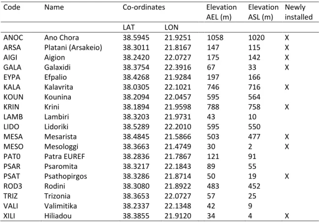
4.1 Locations and characteristics of permanent GNSS stations used in PaTrop ... 34

4.2 CRL tropospheric solution settings ... 35

5.1 WRF parameterization options used for the PaTrop sensitivity analysis ... 42

5.2 Pearson Correlation Co-efficient results for all schemes (17/6-29/6/2016) ... 44

5.3 Mean Bias results for all schemes (17/6-29/6/2016) ... 44

5.4 Mean Average Bias results for all schemes (17/6-29/6/2016) ... 45

5.5 RMSE results for all schemes (17/6-29/6/2016) ... 45

5.6 Absolute elevation differences and MAE at 16 GNNS nearest WRF grid points for 5 topographical datasets (d04). ASTER 1s global GDEM v2 is used as the reference map. ... 48

5.7 Pearson Correlation Co-efficient results for MOD5 with 5 topograpical sets (17/6-29/6/2016) ... 50

5.8 Mean Absolute Bias results for MOD5 with 5 topograpical sets (17/6-29/6/2016)... 50

5.9 Locations and characteristics of WRF grid point nearest to GNSS station (ASTER 1s DEM) ... 51

6.1 Statistical indices of complete WRF ZTS vs. GNSS ZTD time series – Jan-Dec 2016 ... 55

6.2 Seasonal statistical indices of WRF ZTS vs. GNSS ZTD time series – 2016 ... 58

6.3 σ values within error range – S1 ... 61

6.7 σ values within error range – WRF vs. PAT0 EUREF solution... 70

6.8 Comparison of seasonal statistical indices of WRF vs. EUREF and WRF vs. CRL ZTD time series –2016 ... 70

7.1 Dates of Sentinel-1 interferograms examined, corresponding WRF vs. GNSS ZTD average bias differences (Δbias), and RMS and SD differences between original and corrected interferograms ... 126

(10)

viii

List of Figures

1.1 Geophysical processes that affect geodetic observations as a function of spatial and

temporal scale ... 4

1.2 Simplified geology and the fault network in the Corinth Rift . ... 6

1.3 Gulf of Corinth: Velocities for the period 2017-2018 and focal mechanisms 2003-2018 ... 7

2.1 Schematic presentation of individual slant path delays (SPDs) from three GNSS satellites and their mapping to zenith total delay (ZTD) ... 12

2.2 Main GNSS positioning techniques used ... 14

2.3 Crustal deformation monitoring with InSAR... 20

2.4 Tropospheric delay estimates for different correction methods ... 23

3.1 Physical processes mathematically modelled in NWP forecasting models ... 25

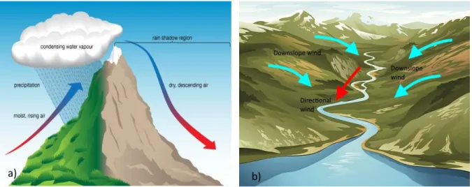
3.2 Effects of topography on local wind patterns ... 29

4.1 Map of the PaTrop study area, Western GoC. ... 32

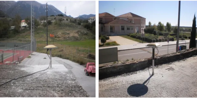
4.2 Photos of newly installed PaTrop GNSS permanent stations in Kalavrita and Mesologgi ... 33

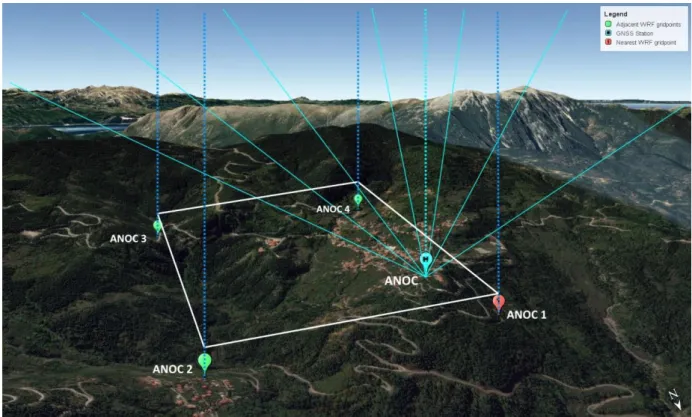
4.3 Example of GNSS-WRF geometry for ANOC Station ... 37

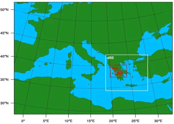
5.1 Map showing the four nested domains (d01-d04) used for WRF weather re-analysis over the Western GoC . ... 39

5.2 RMSE distribution for each model configuration at the 16 stations ... 46

5.3 Distribution of model validation metrics (MAB, RMSE and PPC) per station elevation h – MOD5 ... 47

5.4 Map of domain 4 showing elevation differences: a) GTOPO 30s minus ASTER 1s DEM opt3; b) ASTER 1s DEM opt1 minus ASTER 1s DEM opt3 . ... 49

6.1 Underlying topography of domain 4, ASTER 1s DEM opt4 ... 54

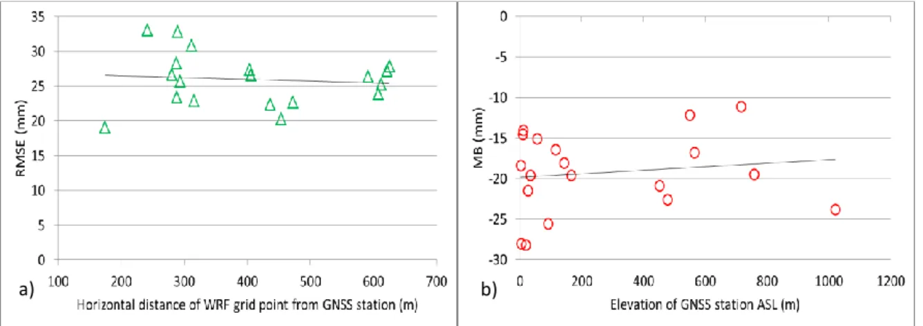
6.2 Plots of: (a) RMSE vs. horizontal distance s between WRF grid point and GNSS station; (b) MB vs. GNSS station elevation h. ... 56

6.3 Distribution of validation metrics (MAB, RMSE and PPC) per station elevation h ... 57

6.4 Monthly variability of MAB at the 19 PaTrop stations, classified per terrain type . ... 59

6.5 Distribution of validation metrics (MAB, RMSE and PPC) per station elevation h, and season (S1-S4) ... 60

6.6 Absolute bias plot for all stations, season S1 ... 62

(11)

ix 6.11 Bias plots of WRF vs. EUREF and WRF vs. CRL ZTDs at PAT0 station ... 69 6.12 Graph of WRF vs. GNSS ZTD time series (top); graph of WRF vs. METEO surface

temperature Ts and surface relative humidity RH (middle); graph of WRF vs. METEO surface pressure at sea level Ps plus wind distribution (bottom). KALA station . ... 73 6.13 Graph of WRF vs. GNSS ZTD time series (top); graph of WRF vs. METEO surface

temperature Ts and surface relative humidity RH (middle); graph of WRF vs. METEO surface pressure at sea level Ps plus wind distribution (bottom). ANOC station ... 74 6.14 Graph of WRF vs. GNSS ZTD time series (top); graph of WRF vs. METEO surface

temperature Ts and surface relative humidity RH (middle); graph of WRF vs. METEO surface pressure at sea level Ps plus wind distribution (bottom). PAT0 station . ... 75 6.15 Maps of water vapour mixing ratio at eta level 6 as calculated by the WRF re-analysis

in 3h intervals . ... 77 6.16 Maps of water vapour mixing ratio at eta level 6 as calculated by the WRF re-analysis

in 3h intervals . ... 78 7.1 Example of producing a differential ZTD map from the subtraction of two single ZTD

maps, produced with WRF at the times of InSAR acquisitions ... 82 7.2 Example of atmospheric correction of an interferogram (18/9-30/9, track 80) ... 82 7.3 Coherence maps for Sentinel-1 ascending track 175 (left) and descending track 80 (right),

over the extended western GoC area ... 85 7.4 Wrapped interferogram from SAR acquisitions on 30/09/2016 and 06/10/2016, track 175

in radar geometry (left). Corresponding WRF-derived wrapped differential LOS delay map (right) ... 86 7.5 Wrapped interferogram from SAR acquisitions on 30/09/2016 and 06/10/2016, track 175

in radar geometry (left). Corresponding residual map after subtraction of WRF-derived wrapped differential LOS delay map from the interferogram (right) ... 87 7.6 Wrapped interferogram from SAR acquisitions on 30/09/2016 and 24/10/2016, track 175

in radar geometry (left). Corresponding residual map after subtraction of WRF-derived wrapped differential LOS delay map from the interferogram (right) ... 89 7.8 Wrapped interferogram from SAR acquisitions on 30/09/2016 and 05/11/2016, track 175

in radar geometry (left). Corresponding residual map after subtraction of WRF-derived wrapped differential LOS delay map from the interferogram (right) ... 91

(12)

x 7.10 Wrapped interferogram from SAR acquisitions on 06/10/2016 and 24/10/2016, track 175

in radar geometry (left). Corresponding residual map after subtraction of WRF-derived wrapped differential LOS delay map from the interferogram (right).. ... 93 7.12 Wrapped interferogram from SAR acquisitions on 06/10/2016 and 11/12/2016, track 175

in radar geometry (left). Corresponding WRF-derived wrapped differential LOS delay map (right) ... 104

(13)

xi 7.23 Wrapped interferogram from SAR acquisitions on 25/08/2016 and 18/09/2016, track 80

in radar geometry (left). Corresponding residual map after subtraction of WRF-derived wrapped differential LOS delay map from the interferogram (right).. ... 117

(14)

xii 7.36 Wrapped interferogram from SAR acquisitions on 18/10/2016 and 24/10/2016, track 80

in radar geometry (left). Corresponding residual map after subtraction of WRF-derived wrapped differential LOS delay map from the interferogram (right).. ... 125 7.44 Correlation of RMS reduction between original and corrected interferograms and

Δbias ... 127 7.45 Correlation of SD reduction between original and corrected interferograms and

Δbias ... 128 7.46 Correlation of % SD reduction vs. % RMS reduction for the 20 cases studied ... 128

(15)

xiii

Abbreviations and Acronyms

APS Atmospheric Phase Screen

ASTER Advanced Spaceborne Thermal Emission and Reflection Radiometer CDDIS Crustal Dynamics Data Information System

CPU Central Processing Unit CRL Corinth Rift Laboratory DEM Digital Elevation Model

DLR Deutsche Lebensmittel Rundschau DEM Digital Elevation Model

DORIS Doppler Orbitography and Radio-positioning by Integrated Satellite DWD Deutscher Wetterdienst

ECMWF European Centre for Medium-Range Weather Forecasts EPN European Processing Network

ESA European Space Agency GAM Global Atmospheric Model GoC Gulf of Corinth

GGOS Global Geodetic Observing System GMF Global Mapping Function

GNSS Global Navigation Satellite System GPS Global Positioning System

GPT Global Pressure and Temperature model GRNET Greek Research and Technology Network HPC High Performance Computer

IGS International GNSS Service IWV Integrated Water Vapour JPL Jet Propulsion Laboratory

(16)

xiv LAGEOS Laser GEOdynamics Satellite

LAM Limited-Area Model LEO Low Earth Orbit LOS Line-of-Sight

MERIS MEdium Resolution Imaging Spectrometer MODIS Moderate Resolution Imaging Spectroradiometer NCEP National Centers for Environmental Prediction NGSLR Next Generation Satellite Laser Ranging NWP Numerical Weather Prediction

PPP Precise Point Positioning PWV Precipitable Water Vapour SAR Synthetic Aperture Radar SGP Space Geodesy Project

SINEX Solution Independent Exchange format SRTM Shuttle Radar Topography Mission SLR Satellite Laser Ranging

TRF Terrestrial Reference Frame USGS United States Geological Survey VLBI Very Long Baseline Interferometry VMF Vienna Mapping Function

WRF Weather Research and Forecasting Model ZHD Zenith Hydrostatic Delay

ZTD Zenith Total Delay ZWD Zenith Wet Delay

(17)

(18)

1

1. Introduction

1.1 Background

Space geodesy techniques (SAR interferometry and GNSS) have recently emerged as an important tool for mapping regional surface deformations due to tectonic movements. A limiting factor to this technique is the effect of the troposphere, as horizontal and vertical surface velocities are of the order of a few mm yr-1, and high accuracy (to mm level) is essential. The troposphere introduces a path delay in the microwave signal, which, in the case of GNSS Precise Point Positioning (PPP), can nowadays be successfully removed with the use of specialized mapping functions [Bevis et al., 1992; Boehm et al., 2006a; Tesmer et al., 2007; Bock et al., 2016]. Moreover, tropospheric stratification and short-wavelength spatial turbulences produce an additive noise to the low amplitude ground deformations calculated by the (multitemporal) InSAR methodology. InSAR atmospheric phase delay corrections are much more challenging, as opposed to GNSS PPP, due to the single pass geometry and the gridded nature of the acquired data. Several methods have been proposed, including local atmospheric data collection [Delacourt et al., 1998], Global Navigation Satellite System (GNSS) zenithal delay estimations [Williams et al., 1998; Webley et al., 2002; Li et al., 2006a; Onn and Zebker, 2006], satellite multispectral imagery analysis [Li et al., 2006b], assimilation of meteorological data in atmospheric models [Wadge et al., 2002; Puysségur et al., 2007] and empirical phase/topography estimations [e.g., Wicks et al., 2002; Biggs et al., 2007; Cavalié et al., 2008; Lin et al., 2010; Bekaert et al., 2015b]. These methods have their limitations, as they rely either on local data assimilation, which is rarely available, or on empirical estimations which are difficult in situations where deformation and topography are correlated. Thus, the precise knowledge of the tropospheric parameters along the propagation medium is extremely useful for the estimation and minimization of atmospheric phase delay, so that the remaining signal represents the deformation mostly due to tectonic or other geophysical processes. In fact, recent studies [Doin et al., 2009; Jolivet at al., 2011, 2014; Kinoshita et al., 2012; Bekaert et al., 2015a] have investigated this trend by calculating tropospheric delays from the output of local or global weather models. However, the low resolution and the generic configuration of the models used have, so far, inhibited the full exploitation of this method.

On the other hand, the same remote sensing techniques used by geophysicists for measuring crustal deformations and other geological phenomena, can provide very useful information of meteorological and climatological interest. In fact, if the same path delay due to the water vapour content in the troposphere can be accurately estimated, it can be used (as Integrated Water Vapour or IWV) in numerous meteorological applications, from assimilation into weather forecasting models [e.g., Poli et al., 2007; Moll et al., 2008; Schwitalla et al., 2011; Szintai and Mile, 2015] to mapping of the 3D distribution of water vapour in the atmosphere [e.g., Wang et al., 2007; Flores et al., 2008; Shangguan et al., 2013]. For example, GNSS is now an established atmospheric observing system, which can accurately sense water vapour, the most abundant greenhouse gas, accounting for 60– 70% of atmospheric warming. In Europe, the application of GNSS in meteorology started roughly two decades ago, and today it is a well-established field in both research and operation [Guerova et al., 2016]. With respect to InSAR, there is still no established methodology which can make use of the

(19)

2 interferometric data for meteorological applications. However, with the onset of new satellite missions (such as the European Space Agency’s Sentinel 1 and 2), it is highly probable that this will happen in the near future, and meteorologists will be able to use data from InSAR imagery to enhance the weather forecasting capabilities of existing Numerical Weather Prediction models. The primary objective of this PhD Thesis is to couple the vertical delay component in GNSS measurements (Zenith Total Delay or ZTD) with the output from a high-resolution meteorological model (WRF), in order to produce a 3D tomography of the troposphere over the study area of the western Gulf of Corinth, Greece. High resolution re-analysis enables a more precise description of local topographic forcings due to orography or land-sea contrasts, and therefore processes strongly forced by topography, such as wind profiles, orographic precipitation and relative humidity, can be represented much more accurately. The model is operated with varying parameterization in order to demonstrate the best possible configuration for our study, with GNSS measurements providing a benchmark of real atmospheric conditions. In the second phase of the study, a novel methodology is developed, in which ZTD maps produced from WRF and validated with GNSS measurements in the first phase of the experiment will be used as a correction method to eliminate the tropospheric effect from selected InSAR interferograms.

1.2 Space Geodesy

Geodesy is the science of the Earth’s shape, rotation, and gravitational field including their evolution in time. In the past, geodesists were using terrestrial measurements, for example land surveying methods or gravity observations, in order to measure the earth’s topographical features or determine the geoid. In recent decades, it has been possible to study the evolution of these “three pillars of geodesy” in time in greater detail, due to the development of space-based geodetic technologies and the realization of a truly global reference system of co-ordinates [Altamimi et al., 1993, 2002]. Space-geodetic techniques which are used to observe the geodetic properties of the Earth include Very Long Baseline Interferometry (VLBI), Satellite Laser Ranging (SLR), Global Navigation Satellite Systems (GNSS) (such as the US Global Positioning System (GPS) or Russian GLONASS), and the French Doppler Orbitography and Radio-Positioning by Integrated Satellite (DORIS) system. These space-geodetic methods provided the basis for the global reference system that is needed in order to assign precise coordinates to terrestrial features and thereby determine how these vary over time. The Terrestrial Reference Frame (TRF) is nowadays the foundation for virtually all airborne, space-based and ground-based Earth observations [Herring, 2007].

Geodetic measurements can be influenced by a variety of Earth processes over a range of spatial and temporal scales, including geophysical processes (crustal deformation associated with plate tectonics, earthquakes, and volcanoes), atmospheric processes (weather and climate dynamics, atmospheric chemistry), oceanic and hydrological processes (tides, ocean circulation, motions and mass fluctuations of glaciers and ice shelves, hydrology and continental water storage). Space geodesy methods have been proven as an invaluable tool for monitoring these diverse processes, as they have provided integrated and geo-referenced sets of observations on global to regional spatial scales with high spatial and temporal resolution. For example, since the end of the last century, VLBI and GNSS have been playing an important role to accurately measure crustal deformation due to

(20)

3 tectonic plate movements with a precision of centimetres to sub-millimetres [e.g. Tralli et al., 1988; Larson and Agnew, 1991; Segall and Davis, 1997; Argus et al., 1999; Larson et al., 2003]. Other geophysical applications of space geodesy include [Blewitt, 2007]:

 GNSS seismology, e.g. interseismic strain accumulation by tracking the relative positions between networks of GNSS stations in and around plate boundaries [Kreemer at al., 2003, 2006b], postseismic processes and rheology of the Earth’s topmost layers, by inverting the decay signature of GNSS station positions in the days to decades following an earthquake [Pollitz, 1997; Kreemer et al., 2006a], seismic waves observations with GNSS [Nikolaidis et al., 2001;] etc.

 Magmatic processes, by measuring time variation in the position of stations located on volcanoes or other regions of magmatic activity, such as hot spots. [Beauducel et al., 2000; Hooper et al., 2004; Lundgren et al., 2004].

 Rheology of the Earth’s mantle and ice-sheet history, by measuring the vertical and horizontal velocities of GNSS stations in the area of postglacial rebound (glacial isostatic adjustment) [Lidberg et al., 2007; Sella et al., 2007], or time-variable gravity [Cox and Chao, 2002; Cheng and Tapley, 2004; Paulson et al., 2007; Tamisiea et al., 2007].

 Mass redistribution in the Earth’s fluid envelope (allowing for the study of atmosphere– hydrosphere–cryosphere–solid-Earth interactions), mostly by means of SLR, such as measuring the time variation in Earth’s shape, the velocity of the solid-Earth centre of mass [Watkins and Eanes, 1997; Ray, 1998; Chen et al., 1999], Earth’s gravity field [Nerem et al., 1993; Gegout and Cazenave, 1993; Cheng and Tapley, 1999, 2004], and Earth’s rotation in space by SLR determination of the exchange of angular momentum between the solid Earth and fluid components of the Earth system [Chao et al., 1987].

 Global change in sea level, by measuring vertical movement of the solid Earth at tide gauges, by measuring the position of space-borne altimeters in a global reference frame, and by inferring exchange of water between the oceans and continents from mass redistribution monitoring.

 Hydrology of aquifers by monitoring aquifer deformation inferred from time variation in 3-D coordinates of a network of GNSS stations on the surface above the aquifer.

 Providing a global reference frame for consistent georeferencing and precision time tagging of nongeodetic measurements and sampling of the Earth, with applications in seismology, airborne and space-borne sensors and general fieldwork. [Altamimi et al., 2002; Altamimi, 2005].

(21)

4

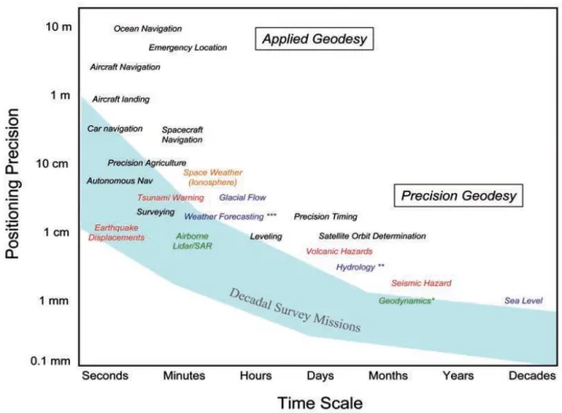
* Plate motion, plate deformation, mountain building, mass transport, ice-sheet changes ** Vertical surface motion from GNSS/GPS and InSAR for ground water management

*** Water vapour and other meteorological information from GNSS/GPS ground stations and radio occultations in space

Figure 1-1. Geophysical processes that affect geodetic observations as a function of spatial and temporal scale (Source: National Research Council. Precise Geodetic Infrastructure: National Requirements for a Shared Resource. Washington, DC: The National Academies Press, 2010).

The required precision for each of the current geodetic applications as a function of the time interval to which they refer is illustrated in Figure 1-1. It is seen that the most demanding applications at the shortest time intervals include GNSS seismology and tsunami warning systems, whereas at the longest time intervals, the most demanding applications include sea level change and geodynamics. Consistency in connecting the longest to the shortest time scales requires an accurate and stable global terrestrial reference frame, which supports the demanding requirements of the geodetic infrastructure. As a general rule, estimation of GNSS station velocity can be achieved with precision < 1 mm yr-1 using > 2.5 years of continuous data [Blewitt, 2007].

An equally important remote sensing technology for studying geophysical phenomena is Synthetic Aperture Radar (SAR), an active radar system mounted on satellites, which transmits microwaves and receives the scattered signals back from the Earth’s surface. Although not a space geodesy method in the narrow sense, SAR observation has been used to monitor many of the

(22)

5 aforementioned processes with great success. During the past two decades, SAR Interferometry (InSAR) has evolved into an established method for measuring:

 Surface deformations associated with earthquakes [e.g. Massonnet and Feigl, 1995; Delacourt et al., 1997; Delouis et al., 2002; Feigl et al., 2002], volcanic activities [e.g. Pritchard and Simons, 2002; Sykioti et al., 2003; Pedersen and Sigmundsson, 2006], land subsidence and uplift [e.g. Massonnet et al., 1997; Carnec et al., 1999; Bawden et al., 2001; Carbognina et al., 2004] and landslides [e.g. Colesanti et al., 2003; Catani et al., 2005].  Land topography at high spatial and vertical resolution, producing precise topographic maps

of both the Earth and Venus [Meyer and Sandwell, 2012].

 Glacier and ice sheet dynamics [e.g. Goldstein et al., 1993; Joughin et al., 1996a; Mohr et al., 1998; Gray et al., 2001].

 Hydrological parameters, such as soil moisture content [e.g. Gabriel et al., 1989; Nolan et al., 2003; Makkearson et al., 2006] and inland water level variations [Alsdorf et al., 2000; Romeiser et al., 2007].

In fact, the combination of high spatial resolution InSAR methodology with high temporal resolution GNSS point measurements produces even better results, with respect to most of these geophysical parameters, and in recent years many studies are exploiting this method to potentially map highly accurate deformations (i.e. at sub-centimetre levels) [Wang and Wright, 2012; Walters et al., 2014; Ozawa et al., 2016].

Space geodesy is revolutionizing the way that environmental parameters are being monitored and is increasing our understanding of the complex Earth system. At the same time, it contributes to mitigating the impact of major geohazards, such as earthquakes, volcanic eruptions, landslides, tsunamis, hurricanes, floods and extreme weather.

1.3 The Corinth Rift Laboratory (CRL)

The Gulf of Corinth (GoC) is known as one of the most active intra-continental rifts in the world. Separating continental Greece to the North from the Peloponnese to the South, the 120 km long structure has been long identified as a site of intense geophysical activity. Geodetic studies conducted during the past 20 years based on GNSS and InSAR observations have revealed North-South extension rates up to 1.5 cm yr-1 [Briole et al., 2000; Avallone et al., 2004], one of the highest worldwide. The Gulf of Corinth also shows one of the highest seismicity rates in the Euro-Mediterranean region, having produced a number of strong earthquakes in recent years: Alkyonides (1981, M=6.7), Galaxidi (1992, M=5.8), Aigio (1995, M=6.2), and Efpalio (2010, M=5.3) (Figure 1-3). The Gulf of Corinth belongs to the general tectonic region of the Eastern Mediterranean, where dynamics are complex. The dominant characteristic of the region is the subduction of the African and Anatolian plates along the Hellenic Arc, which controls the rifting as a result of the extension in the back-arc region of the Aegean subduction zone, enhanced by the interaction with the Western tip of the North Anatolian Fault [Armijo et al., 1996, 2004; Jolivet, 2001; Hubert-Ferrari et al., 2003; Kokkalas et al., 2006; Reilinger et al., 2010; Pérouse et al., 2012].

(23)

6 Figure 1-2. Simplified geology and the fault network in the Corinth Rift. Faults in red (high strain setting) indicate the currently active Rift zone and faults in black (low strain setting) the currently inactive Rift zone. (Source: Michas et al., 2015).

With regards to the fault structure, The Gulf of Corinth appears as an asymmetrical rift [Bernard et al., 2016], with the most active normal faults dipping north, resulting in the long term subsidence of the northern coast and a general uplift of the southern coast (northern Peloponnese) [Armijo et al., 1996; Palyvos et al., 2007; Elias et al., 2009]. The fault system consists of a large number of offshore and on-shore (well visible at the surface) long faults, most of them striking E-W (e.g. Eliki, Kamari, Psathopyrgos, Aigio, Trizonia, Eratini), along which large earthquakes occur. The stratigraphy reflects the present and quaternary tectonics of the rift [Bernard et al., 2016]: to the north of the gulf, the mountainous, subsiding Hellenides limestone nappes are outcropping almost everywhere along the rift; to the south, these nappes are mostly covered by a thick (several hundreds of meters) conglomerate layer, and only outcrop on the footwall of the southern active faults [e.g., Armijo et al., 1996; Ghisetti and Vezzani, 2004]. Along the coastline, and offshore, on the walls of the normal faults, the conglomerates are covered by finer, recent deposits (sands and clay), up to 150 m thick in the Aigion harbour [Pitilakis et al., 2004; Cornet et al., 2004b]. The fault structure and the geology of the Gulf of Corinth are illustrated in Figure 1-2.

In this context, the Corinth Rift Laboratory (CRL) has been established in recent years, as a large international research effort bringing together scientists from a number of European countries and institutions [Cornet et al., 2001, 2004a; Web: http://www.crlab.eu].

(24)

7 Figure 1-3. Gulf of Corinth: Velocities for the period 2017-2018 and focal mechanisms 2003-2018 (Source: crlab.eu).

The CRL project has been studying the short and long term mechanics of the normal fault system, with ongoing research mostly focused on the western part of the rift, as recent tectonic activity is shown to be migrating westwards based on a number of indicators [Bernard et al., 2016]: (1) local strain rates are higher (reaching a maximum of 16 mm yr-1 at the western tip); (2) microseismic activity is more prominent; (3) this area has not experienced destructive (M>5.5) earthquakes in the last century; (4) in the past 40 years, seismic activity has been migrating westwards, with the last major earthquake occurring in 1995 at Aigio (M=6.2) [Tselentis et al., 1996; Bernard et al., 1997]. Tectonic studies in the area of the Western Gulf of Corinth have produced detailed maps of the main presently active faults, both onshore [e.g. Flotté et al., 2005; Palyvos et al., 2005, 2008; Ford et al., 2009, 2013; Papanikolaou et al., 2009; Michas et al., 2015], and offshore [Stefatos et al., 2002; Sakellariou et al., 2003, 2007; Bell et al.,2009; Taylor et al., 2011; Charalampakis et al., 2014; Beckers et al., 2015]. At the same time, the monitoring network of CRL is steadily expanding, and currently includes seismometer arrays (both onshore and submarine), strain gauges, tidal gauges, inclinometers, as well as a dense array of 25 permanent GNSS stations, providing continuous geodetic measurements in the area (Figure 1-3). In fact, the combination of long-term permanent and campaign GNSS observations with active satellite observations (InSAR), processed with advanced differential interferometry methodologies (i.e. PSI and SBAS) is capable of providing precise geodetic measurements at high resolution, thus greatly enhancing the knowledge of local crustal deformations with multiple benefits for monitoring co-seismic, post-seismic, as well as aseismic discontinuities.

(25)

8

1.4 Rationale – Objectives

In the context of CRL, the need for high-quality satellite data is emphasized, as it can provide valuable information about crustal deformations and fault dynamics. Meteorology is therefore an integral part of the monitoring effort, as the precise knowledge of the tropospheric state can remove a main source of error from the data which is the delay due to the atmospheric refraction of the signal. On the other hand, the synergy of remote sensing techniques such as GNSS and InSAR used for geodetic measurements with meteorological applications can provide very useful information of meteorological and climatological interest. It is, for example, highly possible that in the near future, InSAR near real-time data will be assimilated in weather forecasting models for improving their predictions, in the same way that GNSS data are currently being used.

With this in view, the current PhD Thesis aims to investigate the extent to which a high-resolution weather model, such as WRF, can produce detailed tropospheric delay maps of the required accuracy, by coupling its output (in terms of Zenith Total Delay or ZTD) with the vertical delay component in GNSS measurements. The model initially is operated with varying parameterization in order to demonstrate the best possible configuration for our study, with GNSS measurements providing a benchmark of real atmospheric conditions. In the next phase, the two datasets (predicted and observed) are compared and statistically evaluated for a period of one year, in order to investigate the extent to which meteorological parameters that affect ZTD can be simulated accurately by the model, under different weather conditions. Finally, a novel methodology is tested, in which ZTD maps produced from WRF and validated with GNSS measurements in the first phase of the experiment will be used as a correction method to eliminate the tropospheric effect from selected InSAR interferograms.

(26)

9

2. Tropospheric Effects in GNSS and InSAR and Current Correction

Methods

2.1 Neutral Atmospheric Delay in Space Geodesy Techniques

The Earth’s neutral atmosphere introduces a propagation delay, due to refraction, in all space geodetic techniques which use microwave signals at frequencies ranging from 300 MHz to 300 GHz. Atmospheric refraction is mainly caused by the spatial and temporal variations of vapour content in the lower atmosphere (troposphere), and it is the principal error source in space geodesy applications such as GNSS [Solheim et al., 1999], VLBI [Treuhaft and Lanyi, 1987], Satellite Altimetry [Desportes et al., 2007], and Interferometric Synthetic Aperture Radar (InSAR) [Hanssen, 2001; Li et al., 2005; Onn and Zebker, 2006]. In this chapter, the tropospheric effect in GNSS and InSAR measurements detecting crustal deformations is discussed and current correction techniques are presented. On the other hand, the “noise” effect of the atmospheric water vapour in geodetic measurements can also be regarded as a “signal” in meteorological terms [Bevis et al., 1992], and therefore its precise determination can be useful in a number of associated applications which are also discussed.

2.2 Tropospheric Effects in GNSS Measurements

2.2.1 Theory of Refractivity and Calculation of Zenith Hydrostatic Delay and Zenith Wet

Delay

Global Navigation Satellite Systems (GNSS) is a well-established and highly accurate geodetic technique which allows us to monitor crustal deformations at the millimetre level. The first system of its kind, known as GPS (Global Positioning System), was initially operated by the U.S. Air Force and became available for civilian use in the 1980s, currently consisting of 32 satellites in medium Earth orbit. In recent years, additional constellations have become operational, such as the Russian GLONASS, the European GALILEO, and the Chinese Beidou, all with global coverage.

GNSS signals emitted from satellites to ground receivers are delayed and bent when propagating through the atmosphere (Figure 2-1). The upper part of the atmosphere (ionosphere) is a dispersive medium, and therefore its first order delay effect (phase advance), which is on the order of 1-50 m, can be eliminated by combining observations from two GNSS L-band frequencies in the range from 1.16 to 1.61 GHz [Spilker, 1978; Ware et al., 1996]. The remaining ionospheric effect due to higher‐ order terms is estimated to be on the order of sub‐millimeter to several centimeters and is usually ignored. However, with recent advancements in GNSS positioning and sub‐centimeter accuracies currently achievable, the correction of this term is becoming increasingly important [e.g. Bassiri and Hajj, 1993; Kedar et al, 2003; Liu et al, 2016].

(27)

10 The delay associated with the lower part of the neutral atmosphere (troposphere) is non-dispersive at GNSS frequencies and cannot be eliminated in a similar way. Within this layer, waves travel slower than in a vacuum (where the refraction index n =1) and also travel in a curved path instead of a straight line [Bevis et al., 1992]. The signal delay is expressed as an equivalent increase in travel path length (ΔL), given by:

∫ ( ) (2.1)

where n(s) is the refractive index as a function of position s along the curved ray path L, and G is the straight-line geometrical path length through the atmosphere (the path that would occur if the atmosphere was replaced by a vacuum).

Equivalently:

∫ [ ( ) ] [ ] (2.2)

where S is the path length along L. The first term on the right is an expression of the slowing effect, and the second term is an expression of bending. The bending term [S – G] is much smaller (about 1 cm or less), for pathswith elevations greater than about 15o.

Equation (2.2) can also be formulated in terms of atmospheric refractivity N, defined as:

( ) (2.3)

The total delay along the zenith path, also known as Zenith Total Delay (ZTD) is expressed as:

( ) ∫ (2.4)

Now N is a function of temperature, pressure, and water vapour pressure, according to the following relationship [Smith and Weintraub, 1953]:

( ) ( ) (2.5)

where P is the total atmospheric pressure (mbar), T is the atmospheric temperature (oK), and Pv is the partial pressure of water vapour (mbar). This expression is considered accurate to about 0.5% under normal atmospheric conditions [Resch, 1984]. A more accurate formula for refractivity in non-ideal gases is provided by Thayer [1974]:

( ) ( ) ₍ ₎ _(2.6)

where k1 = (77.604 ± 0.014) K mbar-1, k2 = (64.79 ± 0.08) K mbar-1, k3 = (3.776 ± 0 .004)x105 K2 mbar-1, Pd is the partial pressure of dry air (mbar) and Zd-1, Zv-1 are the inverse compressibility factors of dry

(28)

11 air and water vapour respectively. Both of these factors, which are corrections for non-ideal gas behaviour, have nearly constant values that differ from unity by a few parts per thousand [Owens, 1967]. The errors in the constants of equation (2.6) limit the accuracy with which the refractivity can be calculated to about 0.02% [Davis et al., 1985].

The first term on the right in equation (2.5) represents the “hydrostatic” delay i.e. the delay which is mainly due to the “hydrostatic” constituents (gases excluding water vapour). It is sometimes referred as “dry” delay, but the term is misleading, as it also includes a significant contribution from water vapour (due to the non-dipole component of water vapour refractivity). The hydrostatic delay forms the largest part of total delay, and can be accurately modelled as it is directly proportional to atmospheric pressure [Saastamoinen, 1972; Davis et al., 1985]. Using the hydrostatic equation and integrating vertically through the atmosphere we obtain for the total hydrostatic zenith delay (ZHD):

( ) ∫ ∫ ( ) (2.7)

where g is the location dependent gravitational constant, Ps is surface pressure (mbar), ρ is air density (g/cm3), and Rd = 2.87 x 106 cm2sec-2K-1 is the gas constant for dry air. Elgered et al. (1991) adopted a model in which the zenith hydrostatic delay (ZHD) is given by:

( ) ( ) ⁄ ( ) (2.8)

where Ps is surface pressure (mbar), and

( ) ( ) (2.9)

accounts for the variation in gravitational acceleration with latitude λ and the height H of the surface above the ellipsoid (in km). Therefore, equations (2.7) and (2.8) demonstrate that a barometric measurement can be used to estimate the zenith hydrostatic delay with high accuracy. If the barometric pressure is known to 1 mbar, zenith hydrostatic delay can be estimated with an accuracy of 2.5 mm [Solheim et al., 1999].

The second and third terms on the right in equation (2.6) represent the “wet” delay i.e. the delay which is due to the water vapour content of the troposphere, and in particular due to the dipole component of its refractivity, which is about 20 times larger than the non-dipole component [Bevis et al., 1992]. Since Zenith Wet Delay (ZWD) is mainly a function of partial water vapour pressure (Pv) and air temperature (T), it can be calculated with a numerical integration through a full atmospheric profile, using these two meteorological parameters together with the two refractivity constants k2’ (K mbar-1) and k3 (K2 mbar-1):

(29)

12 Figure 2-1. Schematic presentation of individual slant path delays (SPDs) from three GNSS satellites and their mapping to zenith total delay (ZTD) (Source: Guerova et al., 2016).

The delay is given in the units of h [Davis et al., 1985]. It is usually adequate to approximate this expression by:

( ) _∫ _(2.11)

Equations (2.10) and (2.11) can be evaluated from profiles of Pv and T provided by meteorological instruments such as radiometers, LIDARs, Fourier transform infrared spectrometers, or radiosondes. However, as these data are rarely available at the GNSS receiver location, and the water vapour profile can fluctuate significantly both in spatial and temporal terms, ZWD is much more difficult to model than ZHD.

Dry air and water vapour are not the only atmospheric constituents which affect the propagation of the GNSS signal. It has been demonstrated that non-gaseous constituents such as hydrometeors (i.e. cloud droplets, rain, hail, snow and graupel), and solid particulates (dust, sand, volcanic ash) can cause phase delays which, depending on the weather conditions, can contribute significantly to the ZTD [Solheim et al., 1999]. Table 2.1 lists typical high values of zenith GNSS propagation delays of different atmospheric constituents, based on the respective refractivities.

(30)

13 Table 2.1: Typical high values of Zenith Total Delay (ZTD) at sea level [Solheim et al., 1999].

Source Magnitude (mm) Scale height

(km)

Dry air 2500 ~8

Water vapour 450 ~2

Hydrometeors 15 variable

Sand/dust 40 ~2

Volcanic ash 0.4 variable

2.2.2 Current Correction Methods – State of the Art

In current GNSS processing software, the tropospheric delay is estimated geometrically, from combining and analysing the signal paths between each satellite and the receiver (Figure 2-1). There are several methods of tropospheric “residual” estimation, e.g. Kalman filter or least square approximation. The tropospheric processing cannot distinguish between the “hydrostatic” and “wet” components, therefore calculates ZTDs not as a sum of ZHD and ZWD, but rather as a sum of an a priori and an estimated tropospheric delay correction. The “a priori” troposphere usually contains the “hydrostatic” component which, under the assumption of hydrostatic equilibrium, is more easily determined from observations or models, plus a default value for the “wet” component. The “residual” term (correction) is estimated from the GNSS solution and represents the remaining ZWD which cannot be modelled a priori and possibly also a small “dry” fraction.

In accurate GNSS applications, a common model for the total slant path delay from the GNSS satellite to the receiver on the surface of the Earth [e.g. Teke et al., 2013] is as follows:

( ) ( ) ( )

( ) [ ( ) ( )] (2.12)

where e and A are the elevation and the azimuth angle towards a specific satellite, ZHD and ZWD are the zenith hydrostatic and zenith wet delays expressed in units of metres, mfh, mfw, mfg are the hydrostatic, wet, and gradient mapping functions, and GN and GE are the components of linear horizontal gradients. The first two terms on the right hand side represent models assuming tropospheric symmetry while the last term may be added in order to estimate a first-order asymmetry in terms of a linear horizontal gradient.

Mapping functions are models which calculate the delay of radio waves from zenith direction down to the observed elevation angle. The Niell Mapping Function (NMF) [Niell, 1996], is a development of the original form by Marini (1972), which incorporates global radiosonde data for the determination of standard profiles. It depends only on the day of year and the site location, but suffers from low

(31)

14 temporal and spatial resolution (1 day/15o in latitude). Subsequent mapping functions, such as the Isobaric Mapping Function (IMF) [Niell, 2000] and the Vienna Mapping Function (VMF1) [Boehm et al., 2006b] make use of Numerical Weather Model (NWM) data and have an improved temporal resolution of 6h. The VMF1 mapping function retrieves data from the European Centre for Medium-Range Weather Forecasts (ECMWF) using a ray-tracing technique, and is found to improve GNSS accuracy, as compared to NMF, by 3mm to 10mm with respect to station height [Boehm et al., 2006b]. Other models such as the Adaptive Mapping Functions (AMF) [Gegout et al., 2011] or the Potsdam Mapping Factors (PMF) [Zus et al., 2014] are also based on the concept of ray-tracing through NWMs. The Global Mapping Function (GMF) is a further development, which results from applying ninth degree spherical harmonics to the VMF1 data. When used in conjunction with the Global Pressure and Temperature model (GPT) [Boehm et al., 2007] it provides an accurate and easy to implement mapping function for most GNSS high precision applications. Weaknesses in GPT/GMF, particularly their limited spatial and temporal variability, have been eliminated by a new, combined model GPT2 [Lagler et al., 2013], and its successor Global Pressure and Temperature 2 wet (GPT2w) [Boehm et al., 2015], having improved capability to determine zenith wet delays empirically. Recently, Landskron and Boehm (2018) have proposed further improvements both to the discrete (VMF1) and empirical (GPT2w) models, called VMF3 and GPT3 respectively, which claim even higher accuracies, especially at low elevation angles.

Figure 2-2. Main GNSS positioning techniques used. PPP uses State Space Representation (SSR) products, such as precise clock, orbits, and ionospheric models from tracking networks (e.g. IGS) that are delivered to the rover via satellite or internet.

(32)

15 Current state of the art in GNSS tropospheric data processing is based on solutions provided by the two predominant GNSS positioning techniques, Precise Point Positioning (PPP) and Relative Positioning (double-differencing). The Precise Point Positioning technique [Zumberge et al., 1997] relies on the trilateration principle to measure distances between a GNSS receiver and a minimum of four satellites, and therefore calculates the receiver’s position in a three-dimensional space, provided that the receiver clock synchronization error is precisely known. Accurate satellite orbit and clock products are provided by the International GNSS Service (IGS), and ionospheric effects are eliminated with the use of a linear LC3 combination (dual-frequency pseudo-range and carrier-phase measurements). Other limiting factors (e.g. tropospheric delay) are either estimated simultaneously as additional unknown parameters, or modelled with the use of specialized functions. Relatively long observation periods are required in PPP applications, and recent studies [e.g. Hesselbarth, 2008] demonstrate that hourly position estimates can reach sub-decimetre accuracy, while observation periods of 4h provide a positioning accuracy at the cm level. On the other hand, Relative Positioning uses double-difference observations from a network of GNSS stations in order to eliminate receiver and satellite clock errors without the use of external products. This makes it possible to segregate the errors attributable to the receiver clock biases from those from other sources, therefore improving the efficiency of the estimation of the integer cycle ambiguity in a carrier phase observation.

Table 2.2: PPP vs. network GNSS processing strategy [Guerova et al., 2016]. Precise point positioning (PPP)

(using raw observations)

Network solution

(using double-differences)

Advantages Small NEQ (clocks & ambiguities pre-eliminated)

Independence of external precise satellite clock products

Station by station individual approach (keeping CPU with increasing number of sites/parameters (higher sampling rate, improved modelling, etc.)

Sensitive to relative models; needs large network

Site-dependent effects do not contaminate other solutions

Correlations between

parameters of all stations taken into account

Sensitive to absolute troposphere

Disadvantages Requires external precise satellite clock

corrections consistent with orbits Large normal equations Requires precise models for

undifferenced observations

Increasing CPU with increase in number of sites/parameters Sensitive to relative model

Figure 2-2 illustrates the two techniques, as compared to absolute point GNSS positioning. Both are capable of producing precise estimates of ZTDs and ZWDs, with short-term RMS errors around 3-4

(33)

16 mm in the ZTD [Guerova et al., 2016]. The choice of technique depends on a number of factors, including the availability of external satellite clock products, the time scale required for the solution (utilisation of real-time, near real-time or final products), CPU availability etc. Table 2.2 lists the strong and weak points of the two GNSS tropospheric processing strategies.

2.2.3 GNSS Meteorology

As already discussed, continuous GNSS observations provide accurate estimations of the tropospheric error which limits geodetic and geophysical applications. At the same time, they are an excellent tool for studying the Earth’s atmosphere, as the observed Integrated Water Vapour (IWV) can be routinely used in a variety of related applications, including numerical weather forecasting, atmospheric research, and space weather applications. The potential of GNSS observations for tropospheric monitoring was initially suggested in the early 90’s [Tralli and Lichten, 1990; Bevis et al., 1992, 1994], when a relationship between the vertically integrated water vapour (IWV) and an observed zenith wet delay was established:

(2.13)

where precipitable water PW is defined as vertically integrated water vapour (IWV) expressed as the height of an equivalent column of liquid water, and the dimensionless quantity Π is given by:

[( ⁄ ) ] (2.14)

[Bevis et al., 1994], where ρ is the density of liquid water, Rv is the specific gas constant for water vapour, and Tm is a weighted mean temperature of the atmosphere defined as:

∫

(2.15)

In fact the relative error in Π closely approximates the relative error in Tm and it has been demonstrated that it is possible to predict Tm from surface temperature observations with a relative RMS error of about 2% [Bevis et al., 1992].

Nowadays, the Zenith Total Delay (ZTD) can be obtained with sub-centimetre accuracy from GNSS data analysis [Byun and Bar-Sever, 2009; Chen et al., 2011; Guerova et al., 2016], and the Zenith Hydrostatic Delay (ZHD) is precisely calculated by means of tropospheric models [e.g. Saastamoinen, 1973], provided that representative meteorological data, either observed near GNSS sites or derived from numerical weather models (NWMs), are available. Therefore the Zenith Wet Delay (ZWD) can be also derived as the difference between ZTD and ZHD [Jin and Luo, 2009], which can then be