the Likelihood of Losses? An Analytical Framework
The MIT Faculty has made this article openly available.
Please share
how this access benefits you. Your story matters.
Citation
Lo, Andrew W. and Thomas J. Brennan. "Do Labrynthine Legal
Limits on Leverage Lessen the Likelihood of Losses? An Analytical
Framework." Texas Law Review 90:1775 (2012).
As Published
http://www.texaslrev.com/90-texas-l-rev-1775/
Publisher
University of Texas School of Law
Version
Author's final manuscript
Citable link
http://hdl.handle.net/1721.1/75358
Terms of Use
Creative Commons Attribution-Noncommercial-Share Alike 3.0
1/36
Do Labyrinthine Legal Limits on Leverage Lessen
the Likelihood of Losses?
An Analytical Framework
†Andrew W. Lo
*and Thomas J. Brennan
**A common theme in the regulation of financial institutions and transactions is leverage constraints. Although such constraints are implemented in various ways—from minimum net capital rules to margin requirements to credit limits—the basic motivation is the same: to limit the potential losses of certain counterparties. However, the emergence of dynamic trading strategies, derivative securities, and other financial innovations poses new challenges to these constraints. We propose a simple analytical framework for specifying leverage constraints that addresses this challenge by explicitly linking the likelihood of financial loss to the behavior of the financial entity under supervision and prevailing market conditions. An immediate implication of this framework is that not all leverage is created equal, and any fixed numerical limit can lead to dramatically different loss probabilities over time and across assets and investment styles. This framework can also be used to investigate the macroprudential policy implications of microprudential regulations through the general-equilibrium impact of leverage constraints on market parameters such as volatility and tail probabilities.
I. Introduction ... 2
II. An Overview of Leverage Constraints and Related Literature ... 6
III. An Analytical Framework... 18
A. Leverage Limits ... 19 † Prepared for the 2012 Texas Law Review Symposium. We thank Allen Ferrell, Henry Hu, David Ruder, Jay Westbrook, and participants at the 2012 Texas Law Review Symposium for helpful comments and discussion and John Gulliver, Adrienne Jack, Christopher Lee, and Morgan MacBride for research assistance. We are also grateful to Jayna Cummings and the Texas Law Review editorial board (Molly Barron, Parth Gejji, Ralph Mayrell, Benjamin Shane Morgan, and Michael Raupp) for many helpful editorial comments. Research support from the MIT Laboratory for Financial Engineering and the Northwestern University School of Law Faculty Research Program is gratefully acknowledged. The views and opinions expressed in this article are those of the authors only and do not necessarily represent the views and opinions of AlphaSimplex Group, MIT, Northwestern University, any of their affiliates and employees, or any of the individuals acknowledged above.
* Charles E. and Susan T. Harris Professor, MIT Sloan School of Management, and Chief Investment Strategist, AlphaSimplex Group, LLC. Please direct all correspondence to: Andrew W. Lo, MIT Sloan School, 100 Main Street, E62–618, Cambridge, MA 02142-1347, (617) 253-0920 (voice), alo@mit.edu (email).
** Associate Professor, School of Law, Northwestern University, 375 East Chicago Avenue, Chicago, IL 60611-3069, t-brennan@law.northwestern.edu (email).
2/36
B. Numerical Examples ... 21
IV. The Dynamics of Leverage Constraints ... 25
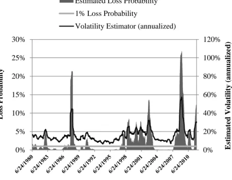
A. Time-Varying Loss Probabilities ... 25
B. An Empirical Illustration with the S&P 500 Index ... 25
C. Correlation and Netting ... 27
V. Qualifications and Extensions... 30
A. Liquidity ... 31
B. Efficacy vs. Complexity ... 32
C. Microprudential vs. Macroprudential Policies ... 35
VI. Conclusion ... 36
I. Introduction
A significant portion of financial regulation is devoted to ensuring capital
adequacy and limiting leverage. Examples include Regulation T,1 the Basel
Accords,2 the National Association of Insurance Commissioners (NAIC)
rules,3 the U.S. Securities and Exchange Commission (SEC) Net Capital
1. Regulation T is the common name for 12 C.F.R. § 220 (2011), which imposes limits on leverage by regulating the credit that may be extended by brokers and dealers. This regulation is discussed in further detail in Part II, infra.
2. The Basel Accords have been promulgated by the Basel Committee on Banking Supervision of the Bank for International Settlements. BASEL COMM. ON BANKING SUPERVISION,BANK FOR INT’L
SETTLEMENTS,BASEL III:AGLOBAL REGULATORY FRAMEWORK FOR MORE RESILIENT BANKS
AND BANKING SYSTEMS (rev. 2011) [hereinafter BASEL III CAPITAL RULES], available at
http://www.bis.org/publ/bcbs189.pdf; BASEL COMM. ON BANKING SUPERVISION,BANK FOR INT’L
SETTLEMENTS, INTERNATIONAL CONVERGENCE OF CAPITAL MEASUREMENT AND CAPITAL
STANDARDS:AREVISED FRAMEWORK (comprehensive ver. 2006) [hereinafter BASEL II], available
at http://www.bis.org/publ/bcbs128.pdf; BASEL COMM. ON BANKING SUPERVISION, BANK FOR
INT’L SETTLEMENTS,INTERNATIONAL CONVERGENCE OF CAPITAL MEASUREMENT AND CAPITAL
STANDARDS (1988) [hereinafter BASEL I], available at http://www.bis.org/publ/bcbs04a.pdf. These
accords establish capital adequacy requirements for banks, and many of the principles of the accords have been adopted in the United States. For a recent discussion of the status of the adoption of the accords in the United States, see STAFF OF THE JOINT COMM. ON TAXATION, 112TH CONG.,NO. JCX-56-11,PRESENT LAW AND ISSUES RELATED TO THE TAXATION OF FINANCIAL INSTRUMENTS
AND PRODUCTS 12 (2011), available at http://www.jct.gov/publications.html?func=download&id=
4372&chk=4372&no_html=1 (explaining that the capital requirements are “generally based on accords promulgated by the Basel Committee on Banking Supervision”); FED. RESERVE SYS.,
COMPREHENSIVE CAPITAL ANALYSIS AND REVIEW:SUMMARY INSTRUCTIONS AND GUIDANCE 4, 18
(2011), available at http://www.federalreserve.gov/newsevents/press/bcreg/bcreg20111122d1.pdf (discussing the Federal Reserve’s adoption of Basel III standards and the expectations those standards place upon banks). The implementation of the accords in the United States is discussed in further detail in Part II, infra.
3. The NAIC promulgates model laws, and these include risk-based capital (RBC) regulations.
See RISK-BASED CAPITAL (RBC) FOR INSURERS MODEL ACT § 312-1 to -10 (Nat’l Ass’n of Ins. Comm’rs 2012) (assuring adequate capitalization of insurance companies by setting corrective actions to be taken if a company reports inadequate capital). These regulations have been adopted as law in many states. See RISK-BASED CAPITAL (RBC)FOR INSURERS MODEL ACT § ST-312-1 to -7 (listing model act adoption by states).
Rule,4 and various exchange-mandated margin requirements.5 These regulations impose a plethora of leverage constraints across banks, broker– dealers, insurance companies, and individuals, all with the same intent: to limit
losses.6 Financial leverage is akin to a magnifying lens, increasing the return
from profitable investments but also symmetrically increasing the losses to
unprofitable ones.7 Therefore, limiting leverage places an upper bound on the
potential losses of regulated entities. However, because it also places an upper bound on the potential profits of such entities, leverage constraints are viewed by financial institutions as boundaries to be tested and obstacles to be
circumvented.8
While this tension is an inevitable consequence of most regulatory supervision, the outcome is generally productive when the leverage constraints operate as they were intended. By preventing institutions and
4. This rule appears in the Code of Federal Regulations as 17 C.F.R. § 240.15c3-1 (2011), and it mandates capital requirements for brokers and dealers. For further discussion of this rule, as well as a description of some recent misinterpretations of the rule by prominent individuals, see Andrew W. Lo, Reading About the Financial Crisis: A Twenty-One-Book Review, 50J.ECON.LITERATURE 151, 175–76 (2012) (discussing various popular misunderstandings in the press and literature about 15c3-1’s role in the financial crisis).
5. For example, the Standard Portfolio Analysis of Risk (SPAN) methodology of the CME Group is “the official performance bond (margin) mechanism of 50 registered exchanges, clearing organizations, service bureaus and regulatory agencies throughout the world.” SPAN, CMEGROUP, http://www.cmegroup.com/clearing/risk-management/span-overview.html.
6. See WALTER W.EUBANKS,CONG.RESEARCH SERV.,R4146,THE STATUS OF THE BASEL III
CAPITAL ADEQUACY ACCORD 1, 7 (2010) (describing the Basel III capital accord’s role as the first
broad international agreement to introduce a leverage ratio requirement in addition to provisions governing the amount of capital banks must hold as a cushion against loss and insolvency); U.S.GEN.
ACCOUNTING OFFICE,GAO/GGD-98-153,RISK-BASED CAPITAL:REGULATORY AND INDUSTRY
APPROACHES TO CAPITAL AND RISK 130–32 (1998) (“The primary purpose of [the SEC net capital
rule] is to ensure that registered broker–dealers maintain at all times sufficient liquid assets to (1) promptly satisfy their liabilities—the claims of customers, creditors, and other broker–dealers; and (2) to provide a cushion of liquid assets in excess of liabilities to cover potential market, credit, and other risks if they should be required to liquidate.”) (footnotes omitted); Mark Mitchell et al.,
Limited Arbitrage in Equity Markets, 57 J. FIN. 551, 559 (2002) (noting that “Regulation T sets boundaries for the initial maximum amount of leverage that investors, both individual and institutional, can employ,” and that “[i]f security prices move such that the investor’s position has less than the required maintenance margin, . . . [the investor] will be required to, at a minimum, post additional collateral or reduce his position so as to satisfy the maintenance margin requirements”);
Risk-Based Capital General Overview, NAT’L ASS’N INS. COMM’RS (2009), http://www.naic.org/d ocuments/committees_e_capad_RBCoverview.pdf (“The NAIC risk-based capital (RBC) system was created to provide a capital adequacy standard that is related to risk . . . .”).
7. Stefan Thurner et al., Leverage Causes Fat Tails and Clustered Volatility 1 (Cowles Found. Discussion Paper No. 1745R, rev. 2011), available at http://papers.ssrn.com/sol3/papers.cfm?abstra ct_id=1963337.
8. See Thomas F. Cosimano & Dalia S. Hakura, Bank Behavior in Response to Basel III: A
Cross-Country Analysis 6 (Int’l Monetary Fund Working Paper WP/11/119, 2011) (discussing how
Basel III requirements could be circumvented and how Basel II was circumvented by banks); Viral Acharya et al., Securitization Without Risk Transfer 3 (Nat’l Bureau of Econ. Research Working Paper No. 15730, Feb. 2010) (“These results suggest, and indeed we document, that the effective leverage of commercial banks was significantly larger than that implied by their on-balance sheet leverage or their capitalization from a regulatory standpoint.”).
individuals from overextending themselves during normal market conditions, these constraints reduce the likelihood of unexpected and unsustainable losses during market dislocations. In doing so, such constraints promote financial stability by instilling confidence in the financial system. The same logic suggests that ineffective constraints and inadequate capital can yield financial instability and a loss of confidence in the financial system. The recent
financial crisis has provided a series of illustrations of this possibility.9
In this paper, we propose that such instability can be attributed to a growing mismatch between static regulatory constraints on leverage and the dynamic nature of market risk in the financial system. Because regulations are slow to change and financial risk can shift almost instantaneously, the likelihood of unintended consequences is virtually certain. Moreover, the breakneck speed of financial innovation and corporate transmutation enables institutions to maneuver nimbly around fixed regulations via regulatory arbitrage. This extreme form of “jurisdiction shopping” allowed AIG Financial Products—one of the most sophisticated and well-funded proprietary trading desks in the world—to be regulated by the Office of Thrift
Supervision (OTS),10 an organization designed to supervise considerably less
complex institutions. If risks can change abruptly, and financial institutions can skirt leverage restrictions via creative financial engineering and corporate restructuring, fixed capital requirements and leverage limits will seem too onerous during certain periods and inadequate during others. This oscillation is due to the cyclical nature of risk in a dynamic (as opposed to a static) economy and is related to—but not the same as—business and credit cycles.
We develop a simple statistical framework for studying capital requirements and leverage constraints that yields several interesting implications for regulating leverage, managing risk, and monitoring financial stability. This framework begins with the observation that all capital adequacy requirements and leverage limits are designed to control the probability of loss
of a certain magnitude.11 This observation implies that five quantities lie at the
heart of such policies: the leverage constraint or capital requirement, the maximum allowable probability of loss, the magnitude of the loss under
9. SeeJOSEPH STIGLITZ, FREEFALL:AMERICA,FREE MARKETS, AND THE SINKING OF THE
WORLD ECONOMY 27 (2010) (describing the freefall of America’s economy in the recent financial
crisis as stemming from deregulation that allowed “the reckless lending of the financial sector, which had fed the housing bubble, which eventually burst”).
10 . According to AIG’s 2007 10-K, “AIG [was] subject to OTS regulation, examination, supervision and reporting requirements.” Am. Ins. Grp., Annual Report (Form 10-K) 13 (Feb. 8, 2008), available at http://www.sec.gov/Archives/edgar/data/5272/000095012308002280/y44393e1 0vk.htm.
11. See infra Part II; Thurner et al., supra note 7, at 3 (“Regulating leverage is . . . good for everyone, preventing [risky] behavior that all are driven to yet none desire.”).
consideration, and the mean and variance of the probability distribution used
to compute the loss probability.12
This result leads to the main thrust of our paper: there is a specific mathematical relation among these five quantities so that if one of them—say, the leverage constraint—is constant over time, then the remaining four must either be fixed as well, or they must move in lockstep as a result of the fixed leverage constraint. This almost-trivial observation has several surprisingly far-reaching implications. As risk varies over time, fixed leverage constraints imply time-varying loss probabilities, in some conditions greatly exceeding the level contemplated by the constraint. Even if risk is relatively stable, as expected returns vary over the business cycle, the probability of loss will also vary and provide incentives for all stakeholders to consider changing the constraint in response. Finally, if asset-return correlations across regulated entities can change over time, as they have in the past, loss probabilities will change as well, spiking during times of financial distress.
These implications underscore the inadequacy of current regulatory restrictions on leverage, which are almost always fixed parameters that require significant political will to change. Although drawing clear bright lines may be good practice from a legal and rule-making perspective, such an approach is not ideal from an economic perspective. Rigid capital requirements and leverage limits may be easier to implement than more flexible and adaptive rules, but they will achieve their intended objectives only in relatively stable environments. Our loss-probability approach provides a systematic framework for integrating microprudential regulation of individual institutions with macroprudential policies for promoting financial stability.
We begin in Part II, An Overview of Leverage Constraints and Related Literature, with a brief overview of existing leverage limits across the banking, brokerage, insurance, and asset-management industries, and provide a short literature review. We introduce our basic framework for determining capital requirements in Part III, An Analytical Framework, by deriving an explicit expression for the leverage constraint as a function of the entity’s asset-return distribution, and provide several numerical examples to develop intuition for the determinants of leverage constraints. In Part IV, The Dynamics of Leverage Constraints, we study the behavior of leverage constraints over time and show that changes in market conditions can change significantly the efficacy of such constraints if they are static. Using the S&P 500 index as an illustrative case, we find that a fixed leverage limit can imply a loss probability of less than 1% in one period and well over 25% in an adjacent period. We
12 . Throughout this paper we consider only probability distributions that are completely determined by their mean and variance. This is the case, for example, for both normal and t distributions, with a specified number of degrees of freedom, and these will be the two main examples we consider. For a description of normal distributions, see 1 WILLIAM FELLER, AN INTRODUCTION
TO PROBABILITY THEORY AND ITS APPLICATIONS, 174 (3d ed. 1968). For a description of t
distributions, see 2 WILLIAM FELLER, AN INTRODUCTION TO PROBABILITY THEORY AND ITS
conclude with some suggestions for improving current leverage-related regulation.
II. An Overview of Leverage Constraints and Related Literature
Investments are often partially financed with borrowed funds. For example, an investor may borrow from his broker to purchase stock, a bank may use amounts deposited with it to invest in various assets, and an individual may secure a mortgage to purchase his home. These and many other borrowing transactions are subject to complex sets of rules that attempt to limit the risk that the borrowed funds will not be repaid. Some rules are imposed directly by governmental regulation, and others are imposed privately by individual parties to transactions or by broad groups engaged in similar types of transactions. Accordingly, the laws and literature on capital requirements and leverage constraints are vast, spanning many contexts, types of financial institutions, and industries. The traditional focus has been on banks, securities firms, and insurance companies. The collection of articles in Capital Adequacy Beyond Basel: Banking, Securities, and Insurance provides an excellent survey of the practices and challenges surrounding capital
adequacy in these industries.13
A theme common to nearly all borrowing rules and regulations is the idea that the borrower should be required to finance a certain amount of the total investment himself without recourse to borrowing. This concept may be expressed as an upper limit on leverage, where leverage is defined as the ratio of the total investment value to the portion of the value financed directly by the borrower. Alternatively, the same idea may be expressed in terms of a minimum margin requirement, where margin is defined as the ratio of the value financed directly by the borrower to the total investment value. The notions of leverage and margin are two sides of the same coin, and, in fact, their numerical values are mathematical reciprocals. Hence, an upper bound on leverage is equivalent to the reciprocal lower bound on margin.
In this section, we consider certain aspects of two prominent sets of regulations—those applicable to lending by broker–dealers and those applicable to banking institutions—to provide context and background for our subsequent modeling and analysis. We start with the well-known example of a governmental margin requirement contained in Regulation T, which
concerns extensions of credit by brokers and dealers to investors.14 The
regulation sets a minimum margin of 50% for the initial purchase of an equity
security by an investor through an account with a broker or dealer.15 The
minimum margin required under Regulation T does not fluctuate with changes
13. CAPITAL ADEQUACY BEYOND BASEL:BANKING,SECURITIES, AND INSURANCE 204(Hal S. Scott ed., 2005).
14. See supra note 1 for the definition of Regulation T.
15. This requirement applies to “margin equity securit[ies],” subject to certain exceptions. 12 C.F.R. § 220.12(a) (2011).
in the market price of a purchased security that continues to be held by the
investor.16 Ongoing maintenance margins that adjust with fluctuations in
value are put in place by private groups and entities, however, and these rules produce a complex tapestry of applicable margin requirements for equity securities. For example, a 25% minimum maintenance margin is required by the Financial Industry Regulation Authority (FINRA)—a private
self-regulatory organization of securities firms17—and individual firms subject
to FINRA rules may, and often do, establish higher maintenance margins.18
The 50% margin requirement of Regulation T does not apply to all investments. For example, the required margin for “exempted” securities and
nonequity securities may be established by a creditor in “good faith.”19 There
are also additional margin rules for investments beyond those covered in
Regulation T, such as those for securities futures.20 Moreover, applicable
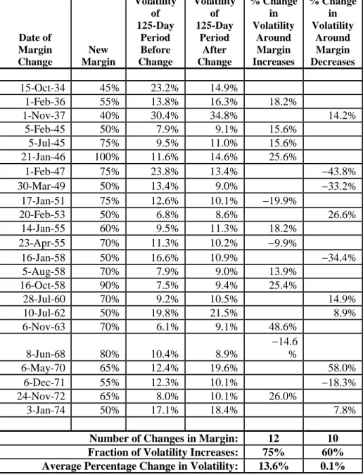
margin requirements have not stayed constant over time but instead have fluctuated significantly. In fact, the initial margin requirement under Regulation T has been as low as 40% and as high as 100% since a limit was
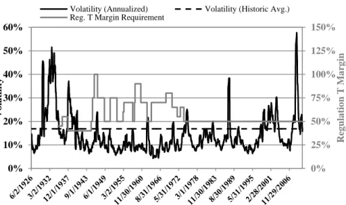
first established in 1934.21 Figure 1 illustrates the margin requirement level as
well as the volatility of equity markets from June 2, 1926 through December 31, 2010. The margin value has been set at 50% since 1974.
16. Id. § 220.3(c)(1) (2011).
17. FIN. IND. REGULATORY AUTH. R. 4210(c) (2010), available at
http://finra.complinet.com/en/display/display.html?rbid=2403&record_id=12855&element_id=9383 &highlight=4210%28c%29#r12855.
18. For example, the TD Ameritrade Margin Handbook states, “[l]ike most brokerage firms, our clearing firm sets the minimum maintenance requirement higher than the 25% currently required by FINRA.” TD AMERITRADE, MARGIN HANDBOOK 5 (2011), available at
https://www.tdameritrade.com/forms/AMTD086.pdf. 19. 12 C.F.R. § 220.12(b) (2011).
20. See 117 C.F.R. §§ 242.400–.406 (2011) (containing regulations of customer margin in the futures context established pursuant to the Securities and Exchange Act of 1934); 17 C.F.R. §§ 41.41–.49 (2011) (containing regulations established pursuant to the Commodities Exchange Act, including customer margin requirements for futures in § 41.42).
21. The data for the historic margin levels under Regulation T were obtained from the New York Stock Exchange (NYSE) Factbook. NEW YORK STOCK EXCHANGE FACTBOOK, http://www.nyxdat a.com/factbook (select the “Margin Debt and Stock Loan” chapter and then select “FRB initial margin requirements”). We use 50% for the 1962 margin level, however, because previous authors have found that the NYSE Factbook has listed this level incorrectly at 90% since 1981. Dean Furbush & Annette Poulsen, Harmonizing Margins: The Regulation of Margin Levels in Stock Index Futures
Markets, 74 CORNELL L.REV. 873, 878 n.25 (1989). The historic volatility is based on 125-day rolling windows of daily market-weighted returns using Center for Research in Securities Prices (CRSP) data. Center for Research in Securities Prices, WHARTON RESEARCH DATA SERVICES, http://wrds.wharton.upenn.edu. For another analysis of historic changes in margin requirements, see generally Peter Fortune, Margin Requirements, Margin Loans, and Margin Rates: Practice and
Date of Margin Change New Margin Volatility of 125-Day Period Before Change Volatility of 125-Day Period After Change % Change in Volatility Around Margin Increases % Change in Volatility Around Margin Decreases 15-Oct-34 45% 23.2% 14.9% 1-Feb-36 55% 13.8% 16.3% 18.2% 1-Nov-37 40% 30.4% 34.8% 14.2% 5-Feb-45 50% 7.9% 9.1% 15.6% 5-Jul-45 75% 9.5% 11.0% 15.6% 21-Jan-46 100% 11.6% 14.6% 25.6% 1-Feb-47 75% 23.8% 13.4% 43.8% 30-Mar-49 50% 13.4% 9.0% 33.2% 17-Jan-51 75% 12.6% 10.1% 19.9% 20-Feb-53 50% 6.8% 8.6% 26.6% 14-Jan-55 60% 9.5% 11.3% 18.2% 23-Apr-55 70% 11.3% 10.2% 9.9% 16-Jan-58 50% 16.6% 10.9% 34.4% 5-Aug-58 70% 7.9% 9.0% 13.9% 16-Oct-58 90% 7.5% 9.4% 25.4% 28-Jul-60 70% 9.2% 10.5% 14.9% 10-Jul-62 50% 19.8% 21.5% 8.9% 6-Nov-63 70% 6.1% 9.1% 48.6% 8-Jun-68 80% 10.4% 8.9% 14.6 % 6-May-70 65% 12.4% 19.6% 58.0% 6-Dec-71 55% 12.3% 10.1% 18.3% 24-Nov-72 65% 8.0% 10.1% 26.0% 3-Jan-74 50% 17.1% 18.4% 7.8%
Number of Changes in Margin: 12 10
Fraction of Volatility Increases: 75% 60%
Average Percentage Change in Volatility: 13.6% 0.1%
Table 1. Changes in Regulation T margin requirements and equity
market volatility before and after each change from 1934 through
1974.22
Figure 1. Margin requirements and 125-day rolling-window volatility
from June 2, 1926 to December 31, 2010. The horizontal dashed line
represents the historic average level of volatility.23
A principal purpose of minimum margin requirements is to protect
lenders from the risk of nonrepayment.24 Accordingly, it may be expected that
minimums would be higher when volatility is higher, and consistent with this expectation, Figure 1 shows clearly that the periods of highest volatility occurred before and after the era of high margin requirements that lasted from the mid-1940s to the early 1970s. We can also analyze the relationship between margins and volatility during the era of high margins.
Table 1 summarizes the change in market volatility from the period 125 days before historic changes in the Regulation T margin requirement to the period 125 days after such changes. There have been twelve increases in the margin requirement since its establishment in 1934, and 125-day volatility has increased in nine of these instances. The average percentage change in volatility around these twelve events was a 13.6% increase. By contrast, there have been ten historic decreases in the requirement, and volatility has decreased in four of these instances, with an average percentage change in volatility of 0.1%. Unfortunately, because of the small data set, the differences between times around margin increases and margin decreases are
23. For explanation of data sources, see supra note 21.
24. See Peter Fortune, Is Margin Lending Marginal?, REGIONAL REV., 3d quarter 2001, at 3, 4 (recounting how one of the main motives for establishing margin requirements in the wake of the 1929 stock market crash was the belief that margin credit led to risky investments and losses for lenders). 0% 25% 50% 75% 100% 125% 150% 0% 10% 20% 30% 40% 50% 60% Reg ula tio n T M a rg in V o la tility
Volatility (Annualized) Volatility (Historic Avg.) Reg. T Margin Requirement
not statistically significant.25 However, the results are suggestive and compatible with the idea that increases in the requirement occur more frequently at times when volatility is increasing, while decreases generally occur at more random times with respect to changes in volatility.
A different type of regulation sets restrictions on the leverage ratio of assets to capital for banking institutions. The applicable definitions of capital and assets are complex and have largely been derived from the principles developed in the accords issued by the Basel Committee on International
Banking Supervision.26 The first accord, known as Basel I, occurred in 1988,
and its principles were made applicable in the United States through
regulations finalized in 1989.27 The second accord, known as Basel II, was
published in 2004, and many of its principles have now been made applicable
in the United States through further regulation.28 To develop an appreciation
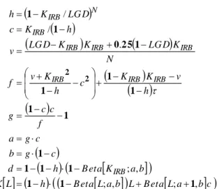
of the complexity of leverage constraints in these various industries, consider Paragraph 624 of Basel II which contains the “Supervisory Formula” used to determine the level of capital for a given bank for purposes of satisfying
capital requirements (see Figure 2).29 Although such formulas may be readily
understood and implemented by financial-engineering experts, they provide little transparency to regulators and policymakers charged with managing systemic risk in the banking industry.
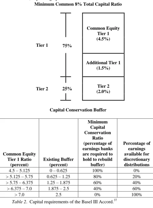
The third accord, known as Basel III,30 was agreed upon in 2010 but has
not yet been implemented in the United States.31 The complexity of its capital
requirements—which incorporate more contingent capital requirements (see Table 2)—will likely be even greater, and will be phased in gradually by various financial institutions over the next few years (see Table 3).
25. For example, the two-sample t-statistic comparing the percentage changes in volatility around increases in margin to those around decreases in margin is , corresponding to a
p-value of 0.26.
26. See generally BASEL COMM. ON BANKING SUPERVISION, CORE PRINCIPLES FOR EFFECTIVE
BANKING SUPERVISION (2011) (setting forth principles to guide countries in the development of
regulations and supervisory practices related to banks and banking systems).
27. BASEL I, supra note 2. The implementation of Basel I into United States regulations can be found in 12 C.F.R. § 3, app. A (2011).
28. BASEL II, supra note 2. The implementation of Basel II into United States regulations can be found in 12 C.F.R. § 3, app. C (2011). According to the Financial Stability Institute, Basel II has been or will be adopted by 112 countries by 2015. FIN.STABILITY INST., OCCASIONAL PAPER NO. 9, 2010
FSISURVEY ON THE IMPLEMENTATION OF THE NEW CAPITAL ADEQUACY FRAMEWORK 6 (2010).
29. BASEL II, supra note 2, at 139.
30. BASEL IIICAPITAL RULES, supra note 2.
31. BASEL COMM. ON BANK SUPERVISION,PROGRESS REPORT ON BASEL IIIIMPLEMENTATION
7–8 (2011); see also Edward Wyatt, Fed Proposes New Capital Rules for Banks, N.Y.TIMES
(Dec. 20, 2011),
http://www.nytimes.com/2011/12/21/business/fed-proposes-new-capital-rules-for-banks.html?_r=2 (reporting that Basel III standards are not expected to be phased in until at least 2016).
L h
B eta
L ab
L B eta
La b
c
K b a K B eta h d c g b c g a f c c g h v K K c h K v f N K LG D K K LG D v h K c LG D K h L K when e K d K K L K K K L when L L S IRB IRB IRB IRB IRB IRB IRB IRB N IRB IRB K L K IRB IRB IRB IRB IRB IRB , ; , ; , ; . / / w here / ] [ / 1 1 1 1 1 1 1 1 1 1 1 1 1 25 0 1 1 1 2 2 Figure 2: Paragraph 624 of the Basel II Accord (2006) specifies the “Supervisory Formula,” which is used to determine the level of capital for a financial institution for purposes of capital-adequacy
supervision.32
In addition to regulatory rules, the Dodd-Frank legislation provides a statutory mandate for general leverage capital requirements and risk-based
capital requirements.33
Although the various Basel Accord rules are complex, the typical capital adequacy requirement for banks has been that capital of specified types must
have a value equal to at least 8% of an adjusted asset number.34 The adjusted
asset number factors are “risk weighting” in the sense that particular assets are assigned weights, with safe assets getting a zero or relatively low number, and
riskier assets getting a relatively high number.35 The weighted average of the
assets is then computed to determine the adjusted asset number.36 The result is
32. BASEL II, supra note 2, at 139.
33. Dodd-Frank Wall Street Reform and Consumer Protection Act (Dodd-Frank Act) § 171, 12 U.S.C. § 5371 (2006 & Supp. IV 2011).
34. See infra Table 2.
35. See BASEL IIICAPITAL RULES, supra note 2; Peter King & Heath Tarbert, Basel III: An
Overview, BANKING &FIN.SERVS.POL’Y REP., May 2011, at 1, 4–5. 36. King & Tarbert, supra note 35, at 2.
a margin/leverage requirement, with a blended requirement level across various assets, depending upon their risk levels.
Minimum Common 8% Total Capital Ratio
Tier 1 Common Equity Tier 1 (4.5%) 75% Additional Tier 1 (1.5%) Tier 2 Tier 2 (2.0%) 25%
Capital Conservation Buffer
Common Equity Tier 1 Ratio (percent) Existing Buffer (percent) Minimum Capital Conservation Ratio (percentage of earnings banks are required to hold to rebuild buffer) Percentage of earnings available for discretionary distributions 4.5 – 5.125 0 – 0.625 100% 0% > 5.125 – 5.75 0.625 – 1.25 80% 20% > 5.75 – 6.375 1.25 – 1.875 60% 40% > 6.375 – 7.0 1.875 – 2.5 40% 60% > 7.0 2.5 0% 100%
Table 2. Capital requirements of the Basel III Accord.37
The capital adequacy regulations contemplate a significant amount of complexity and sophistication in risk-weighted asset calculations. In particular, banks are permitted to use internal models to calculate quantities
such as “value-at-risk” (VaR)38
and to use these quantities in determining the
value of risk-weighted assets.39
While insurance companies face a different set of capital requirements, the motivation for such requirements is similar to that for banks: to reduce the likelihood of defaulting on promised payments to customers. However, Scott E. Harrington has argued that extending the Basel framework to insurance and reinsurance companies is ill-advised because these institutions are less systemically important and face greater market forces that impel them
to maintain adequate capital reserves.40 During the 1991 to 1994 period, U.S.
insurance companies migrated from minimum absolute capital requirements to minimum risk-based capital (RBC) requirements developed by the National
Association of Insurance Commissioners.41 Martin Eling and Ines Holzmüller
provide a useful overview of RBC standards in the United States, Europe, New Zealand, and Switzerland for property–casualty insurers and conclude that there is great heterogeneity in how risk-based capital is defined and the types
of regulations used to ensure capital adequacy (see Table 4).42
The recent financial crisis has taught us that insufficient capital is also problematic for money market funds, pension funds, hedge funds,
governments, and any nonfinancial institution that is a counterparty to
over-the-counter (OTC) derivatives transactions.43 In these cases, the notion
38. See BASEL IIICAPITAL RULES, supra note 2; value-at-risk is a measure of risk that is equal to the level that performance will equal or exceed in all but x% of cases, where x% is a tolerance parameter that must be specified. VaR is defined as the maximum portfolio loss that can occur during a specified period within a specified level of confidence. NEIL D.PEARSON,RISK BUDGETING:
PORTFOLIO PROBLEM SOLVING WITH VALUE-AT-RISK 3–4 (2002).
39. King & Tarbert, supra note 35, at 7.
40 . Scott E. Harrington, Capital Adequacy in Insurance and Reinsurance, in CAPITAL
ADEQUACY BEYOND BASEL, supra note 13, at 87, 88.
41. Id. at 100–01.
42. Martin Eling & Ines Holzmüller, An Overview and Comparison of Risk-Based Capital
Standards, J. INS.REG.,Summer 2008, at31.
43 . See generally Reform of the Over-the-Counter Derivative Market: Limiting Risk and
Ensuring Fairness: Hearing Before the H. Comm. on Fin. Servs., 111th Cong. 10–11 (2009)
(statement of Henry Hu, Director, Div. of Risk, Strategy, and Fin. Innovation, U.S. Sec. & Exch. Comm’n) (explaining that “the recent financial crisis revealed serious weaknesses in the U.S. financial regulation,” including “the lack of regulation of OTC derivatives,” creating risks that “can lead to insufficient capital, inadequate risk management standards, and associated failures cascading through the global financial system”); id. at 10–14, 24–32, 45–46 (discussing approaches to the regulation of nonfinancial entities that use swaps and customized OTC derivatives and the implications of regulation on the behavior of market participants, including financial and nonfinancial institutions); FIN.CRISIS INQUIRY COMM’N,THE FINANCIAL CRISIS INQUIRY REPORT 354 (2011) (describing the market failure immediately following the collapse of Lehman Brothers and noting that “[a]mong the first to be directly affected were the money market funds and other institutions that held Lehman’s $4 billion in unsecured commercial paper,” and that “[o]ther parties with direct connections to Lehman included the hedge funds, investment banks, and investors who were on the other side of Lehman’s more than 900,000 over-the-counter derivatives contracts . . . . The Lehman bankruptcy caused immediate problems for these OTC derivatives counterparties”); id. at 428 (identifying “insufficient capital” as one of the “common risk management failures” that led to the financial crisis); Michael S. Barr, The Financial Crisis and the Path of Reform, 29 YALE J. ON REG.
of liquidity—particularly “funding liquidity”—becomes more relevant, as
Markus Brunnermeier and Lasse Pedersen44 as well as John Dai and Suresh
Sundaresan45 argue. These authors show that during times of financial
distress, insolvency is not the only challenge to financial institutions; the ability to maintain liquidity in the face of forced unwindings can be equally challenging, as we learned in 1998 from the case of Long-Term Capital
Management (LTCM).46
In fact, hedge funds, money market funds, and insurance companies are now often referred to collectively as being part of the “shadow banking system” since they perform many of the same functions as traditional banks but are not subject to the same regulatory supervision and oversight as the banking industry. Moreover, while we have certain indirect measures of the amount of leverage employed by hedge funds and insurance companies and
the illiquidity risk they are exposed to,47 these institutions currently have no
reporting requirements to federal regulators regarding their degree of leverage
91, 94, 104 (2012) (asserting that in the lead up to the financial crisis derivatives were traded “with insufficient capital to back the trades,” and that “[t]he lack of information on derivative exposures led firms to withdraw from counterparties” and to demand “more margin protection from their remaining counterparties, which put further downward pressure on underlying asset prices”); Willa E. Gibson,
Clearing and Trade Execution Requirements for OTC Derivatives Swaps Under the Frank-Dodd Wall Street Reform and Consumer Protection Act, 38 RUTGERS L.REC. 227, 230 (2011) (noting that “[i]n 2009 . . . , 90% of Fortune 500 companies used customized [OTC derivatives],” and describing the Dodd-Frank regulatory approach, whereby “a non-financial entity utilizing OTC derivatives swap contracts for mitigating or hedging risks . . . is exempted from clearing” its customized contracts, and those counterparties who are not exempted are subjected to a bifurcated regulatory approach that “was designed with the expectation that the capital and margin requirements would suffice to manage the systemic as well as counterparty risk that has historically threatened the integrity and stability of the OTC derivatives markets”).
44. Markus K. Brunnermeier & Lasse Heje Pedersen, Market Liquidity and Funding Liquidity, 22 REV.FIN.STUD. 2201, 2201–02 (2009).
45. John Dai & Suresh Sundaresan, Risk Management Framework for Hedge Funds: Role of Funding and Redemption Options on Leverage 1–2 (Mar. 21, 2010) (unpublished manuscript) (on file with author).
46. See generally PRESIDENT’S WORKING GRP. ON FIN.MKTS.,HEDGE FUNDS,LEVERAGE, AND
THE LESSONS OF LONG-TERM CAPITAL MANAGEMENT (1999) (recounting the lessons learned from
the near-collapse of Long-Term Capital Management, including the effects of liquidity shocks on distressed firms).
47. See generally, e.g., Mila Getmansky et al., An Econometric Model of Serial Correlation and
Illiquidity in Hedge Fund Returns, 74 J.FIN.ECON. 529 (2004) (describing measures of illiquidity risk); Monica Billio et al., Econometric Measures of Connectedness and Systemic Risk in the Finance
and Insurance Sectors, 105 J.FIN.ECON.(forthcoming 2012) (describing network measures of systemic risk).
P ha se -i n A rr a nge m ent s (sha d ing i nd ica te s t rans it io n per iods – al l d at es a re a s of 1 Ja nua ry ) 2 0 1 1 2 0 1 2 2 0 1 3 2 0 1 4 20 15 2 0 1 6 2 0 1 7 2 0 1 8 A s o f 1 J a n u a ry 2 0 1 9 L e v era g e R a ti o Su p erv isor y M o n it o ri n g P ar al le l ru n 1 Ja n 2 0 1 3 – 1 J an 2 0 1 7 , D isc lo su re st a rt s 1 Ja n 2 0 1 5 M ig ra ti o n to P il la r 1 M in im u m C o mmon E q u it y C ap it a l R at io 3 .5 % 4 .0 % 4 .5 % 4 .5 % 4 .5 % 4 .5 % 4 .5 % C ap it a l C o n se rv at io n B u ff er 0 .6 2 5 % 1 .2 5 % 1 .8 7 5 % 2 .5 0 % M in im u m c o mmo n eq u it y p lu s ca p it a l c o n se rv a ti o n b u ff er 3 .5 % 4 .0 % 4 .5 % 5 .1 2 5 % 5 .7 5 % 6 .3 7 5 % 7 .0 % Ph ase -i n o f d ed u ct io n s fr o m C E T 1 (i n c lu d in g a mo u n ts ex c ee d in g t h e li mi t fo r DTA s, M SR s an d fi n an ci al s 2 0 % 4 0 % 60 % 80 % 1 0 0 % 1 0 0 % M in im u m T ie r 1 C a p it a l 4 .5 % 5 .5 % 6 .0 % 6 .0 % 6 .0 % 6 .0 % 6 .0 % M in im u m T o ta l C ap it al 8 .0 % 8 .0 % 8 .0 % 8 .0 % 8 .0 % 8 .0 % 8 .0 % M in im u m T o ta l C ap it a l p lu s c o n se rv a ti o n b u ff er 8 .0 % 8 .0 % 8 .0 % 8 .6 2 5 % 9 .2 5 % 9 .8 7 5 % 1 0 .5 % C ap it a l in st ru me n ts th at n o lo n g er q u a li fy a s n o n -c o re T ie r 1 c ap it al o r T ie r 2 c a p it a l P h ase d o u t o v er 1 0 y ea r h o ri zo n b eg in n in g 2 0 1 3 L iq u id it y c o v er ag e ra ti o Ob se rv at io n p er io d b eg in s In tr o d u ce m in im u m st an d ar d Ne t st ab le fu n d in g r at io Ob se rv at io n p er io d b eg in s In tr o d u ce mi n im u m st an d ar d Tabl e 3 . Propos ed phas e-in t im e tabl e f or v ar ious c om ponent s of t he Bas el I II A ccor d.
System RBC standards Solvency II
Self-Regulatory
Framework Swiss Solvency Test 1. General information
Country of application
USA European Union New Zealand Switzerland
Years of introduction 1994 2012 (expected) 1994 2006
Main pillars 1. Rules-based RBC
formula 2. RBC model law on intervention authority 1. Quantitative regulations for capital requirements 2. Qualitative supervisory review 3. Public disclosure 1. Fair Insurance Code 2. Insurance and Savings Ombudsman Scheme 3. Insurance Council’s Solvency Test 1. Principles-based target capital model 2. Risk management report
3. Quality assessment
Regulated companies Insurers (domestic &
foreign); no reinsurers Insurers and reinsurers (domestic & foreign) P&C insurers (domestic & foreign); no life insurers or reinsurers Insurers and reinsurers (domestic & foreign) Consideration of management risk No Rudimentarily addressed by pillar II Yes No Public disclosure requirements
Yes Yes Yes No
2. Definition of capital required
Model typology Static factor model Static factor +
dynamic cash-flow model
Static factor model Static factor +
dynamic cash-flow model
Rules- versus Principles-based
Rules-based Principles-based Principles-based Principles-based
Total balance sheet approach
No Yes Yes Yes
Time horizon 1 year 1 year 1 year 1 year
Risk
measure/calibration
No risk measure Value at risk/99.5%
confidence level
A.M. Best: Expected policyholder deficit S&P: Value at risk
Expected shortfall/99% confidence level Consideration of operational risk Not explicitly (implicit via off-balance-sheet items—R0)
Quantitatively A.M. Best: No
explicit consideration S&P: Quantitatively Qualitatively Consideration of catastrophe
No Yes (as part of
underwriting risk)
Yes Yes
Use of internal models No Appreciated No Appreciated for
insurers; required for reinsurers 3. Definition of available capital
Definition based on market or book values
Book values Market values Market values Market values
Classification of available capital
No Yes (three tiers) No No
Consideration of off-balance-sheet items
No Yes Yes No
4. Intervention
Levels of intervention 4 2 No intervention by
regulator, but market discipline
2
Clarity of sanctions Strict, clear rules Not clear yet No direct sanctions Not clear yet
Table 4. Comparison of risk-based capital standards in property–
casualty insurance companies in the United States, Europe, New
Zealand, and Switzerland.48
and illiquidity.49 Because risk is not static—it is, in fact, determined endogenously by the ongoing interactions of all market participants, as shown
by Jon Danielsson, Hyun Shin, and Jean-Pierre Zigrand50—the lack of
transparency of the shadow banking system makes it virtually impossible for regulators to either anticipate or respond to changes in systemic risk with any degree of precision or speed.
One other strand of literature that is relevant to leverage constraints attempts to quantify the economic cost of insuring the solvency or liquidity of an entity. Its relevance is clear: by measuring the cost of such insurance, we can prioritize the need for capital requirements among the most costly entities. The standard approach is due to Robert C. Merton, who observed that financial guarantees are equivalent to put options on the assets of the insured
entity,51 hence the cost of the guarantee is the market price of the put option or
the production cost of synthetically manufacturing such a derivative contract
by a dynamic portfolio strategy.52 This powerful paradigm provides explicit
valuation formulas for many types of guarantees and has been applied to the
valuation of deposit insurance,53 the management of risk capital in a financial
institution,54 the valuation of implicit government guarantees to Fannie Mae
and Freddie Mac,55 and the measurement of sovereign risk.56 The approach
49. The first leverage and liquidity reporting requirements for hedge fund advisors are scheduled to come into effect for fiscal years ending on or after June 15, 2012. Reporting by Investment Advisers to Private Funds and Certain Commodity Pool Operators and Commodity Trading Advisors on Form PF, Release No. IA-3308, 76 Fed. Reg. 71,128, 71,157 (Nov. 16, 2011); Press Release, Sec. & Exch. Comm’n, SEC Approves Confidential Private Fund Risk Reporting (Oct. 26, 2011), http://www.sec.gov/news/press/2011/2011-226.htm (summarizing the new reporting requirements, including disclosure of leverage and liquidity information for certain hedge funds). In the case of insurance companies, regulation is generally at the state level, but certain companies may be subject to federal regulation for reasons not specifically related to their insurance business. For example, AIG was subject to supervision by the Office of Thrift Supervision until March 2010, and if currently proposed rules are adopted, AIG will be subject to Federal Reserve Board regulation as a systemically important financial institution under the Dodd-Frank Act. Am. Ins. Grp., Annual Report (Form 10-K) 18–19 (2011), available at
http://www.aigcorporate.com/investors/2011_February/December_31,_2010_10-K_Final.pdf. 50. See Jon Danielsson et al., Balance Sheet Capacity and Endogenous Risk 2 (Aug. 2011) (unpublished working paper) (discussing a model for equilibrium and market risk as functions of aggregate bank capital).
51. Robert C. Merton, An Analytic Derivation of the Cost of Deposit Insurance and Loan
Guarantees, 1 J. BANKING &FIN. 3, 4 (1977).
52 . Robert C. Merton, On the Application of the Continuous-Time Theory of Finance to
Financial Intermediation and Insurance, 14 GENEVA PAPERS ON RISK &INS. 225, 228 (1989). 53. Merton, supra note 51, at 8–9.
54. See Robert C. Merton & André Pérold, Theory of Risk Capital in Financial Firms, J.APPLIED
CORP.FIN., Fall 1993, at 17 (defining “risk capital” as the amount invested to insure the firm’s net asset value and demonstrating that the amount of risk capital necessary depends on the riskiness of the net assets and not on the form of financing).
55. Deborah Lucas & Robert McDonald, Valuing Government Guarantees: Fannie and Freddie
Revisited, in MEASURING AND MANAGING FEDERAL FINANCIAL RISK 131, 135 (Deborah Lucas ed., 2010).
taken in these studies is highly complementary to ours. We make use of the same statistical inputs: the probability distribution of asset returns. However, our focus is not on pricing guarantees—which requires more economic structure, such as an equilibrium or arbitrage-pricing model—but on the less ambitious task of relating capital requirements and leverage constraints to other aspects of an entity’s financial condition.
III. An Analytical Framework
If the primary purpose of leverage constraints is to limit the potential losses of an entity, the most natural way to frame such a concept is in terms of loss probabilities. For a given portfolio, define the following quantities:
πt ≡ date-t profit and loss of the portfolio
Kt ≡ date-t assets under management
It ≡ Lt × Kt = leveraged assets, Lt ≡ leverage ratio ≥ 1 Rt ≡ t t I = portfolio return
The probability that this portfolio will lose more than a fraction of its
capital Kt on any date t is given by:
Prob(πt < –δKt) (1)
A leverage constraint can be viewed as an attempt to impose an upper bound on this probability, i.e.,
Prob(πt < –δKt) ≤ γ (2)
for some predefined level of γ, e.g., 5%.57 This expression may also be used to
define the amount of collateral or margin required by a counterparty (such as a broker or supervisory agency) so as to cover a potential loss of up to δKt with probability 1–γ. For larger values of δ, larger potential losses can be covered; for smaller values of γ, the likelihood of coverage is greater.
56. Dale Gray, Modeling Financial Crises and Sovereign Risks, 1 ANN.REV.FIN.ECON.117, 129(2009).
57. The condition in (2) is closely related to the concept of Value-at-Risk (VaR), a measure of risk that is used in many contexts, including banking capital adequacy rules. See supra note 38 and accompanying text. The formula in (2) is thus equivalent to the statement that VaR for the investment portfolio, with specified confidence level γ, is a loss that is no larger than δKt. See, e.g., Risk-Based Capital Guidelines, 12 C.F.R. § 3, app. B (“[E]nsur[ing] that banks with significant exposure to market risk maintain adequate capital to support that exposure.”); Capital Adequacy Guidelines for Banks, 12 C.F.R. § 3, app. C (establishing “[m]inimum qualifying criteria for . . . bank-specific internal risk measurement . . . processes for calculating risk-based capital requirements”).
A. Leverage Limits
An analytic expression for a constraint on leverage Lt corresponding to the upper bound γ may be readily obtained by inverting (2) under the assumption of normality for the portfolio’s profit-and-loss πt:
(3)
1 1 L Lt (4)where is the standard normal cumulative distribution function and
is its inverse.58
Inequality (4) relates the leverage constraint L to four parameters: the loss threshold δ, the expected return μ, and volatility σ, of the portfolio, and the loss probability γ. For a fixed loss probability γ, the leverage constraint is tighter (lower) for higher volatility σ, lower expected return μ, and a smaller loss threshold δ. With the other parameters fixed, a smaller γ implies a more reliable leverage constraint, i.e., one that is more likely to be satisfied. These are the trade-offs that policymakers and regulators must consider when they impose statutory limits on leverage.
A conservative approach to using (4) would be to assume a zero or negative value for the expected return μ (since it is mainly under adverse market conditions that a leverage constraint is most useful). From the financial institution’s perspective, assuming μ = 0 may penalize high-return strategies, but if a portfolio’s expected return is difficult to ascertain ex ante with any degree of precision, an assumption of zero may not be an
58 . The standard normal distribution has mean zero and standard deviation one, and its cumulative probability density is given by
x x x e x d. 2 1 2/2 1 WILLIAM FELLER, AN INTRODUCTION TO PROBABILITY AND ITS
APPLICATIONS 174 (3d ed. 1968).
σ μ δ/L γ σ μ δ/L γ γ σ μ δ/L σ μ δ/L σ μ R δ/L R δK K L R δK π t t t t t t t t t t t t t 1 1 1 Prob Prob Prob Prob 1unreasonable starting point. In such cases, (4) reduces to a particularly simple expression that involves only δ, σ, and γ:
(5)
For more risk-averse financial institutions such as savings and loans, money market funds, and other depository entities, a smaller δ—one commensurate with the lower-volatility assets held by these institutions—is appropriate. More speculative entities such as hedge funds may allow for larger δ, corresponding to more risky portfolio holdings. These risk-dependent considerations can be incorporated directly into the leverage constraint by simply specifying δ in units of return standard deviation: δ = κσ. This specification makes the loss threshold a multiple κ of the standard deviation of the portfolio's return, hence riskier assets will have higher loss thresholds and less risky assets will have tighter thresholds. This risk-sensitive leverage constraint seems to be a more accurate reflection of the motivation underlying such laws.
In this case, the expression for the leverage limit L takes on a particularly transparent form:
(6)
where SR denotes the Sharpe ratio (relative to a 0% risk-free interest rate).59
This version of the leverage constraint states that if leverage does not exceed L , then the probability of a κ-standard-deviation loss of capital is at most γ. Higher Sharpe-ratio strategies will have greater freedom to take on leverage, implying larger values for L . Lower Sharpe-ratio strategies will be more severely leverage-constrained. This relation between Sharpe ratios and leverage is intuitive, but it should be noted that certain illiquid investment strategies may yield inflated Sharpe-ratio estimates due to serial correlation in
their monthly returns.60 These estimates must be adjusted for such effects
before being used to establish leverage contraints.61
59. See William F. Sharpe, The Sharpe Ratio, J.PORTFOLIO MGMT.,Fall 1994, at 49, 50 (“In [the
ex ante version of the Sharpe ratio], the ratio indicates the expected differential return per unit of risk
associated with the differential return.”).
60. See generally Andrew W. Lo, The Statistics of Sharpe Ratios, 58 FIN.ANALYSTS J. 36, 36– 52, (2002). 61. Id.
γ
σ δ L 1 Φ 1
γ
SR, SR μ/σ κ L 1 Φ 1B. Numerical Examples
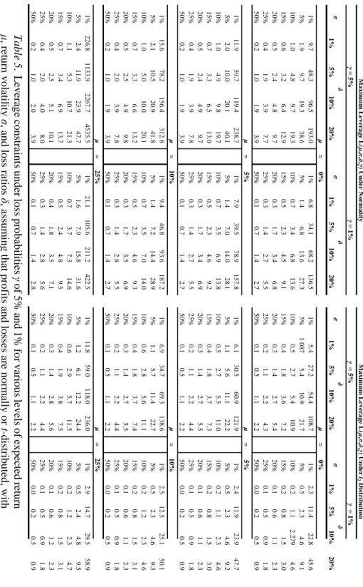
To develop intuition for the leverage constraints (4) and (6), Table 5
reports values of L for a variety of
expected-return/volatility/loss-threshold/loss-probability combinations under normally and t-distributed portfolio returns. The magnitudes of these leverage limits seem broadly consistent with common intuition for various financial institutions. For a loss ratio of, say, δ = 20% and annual volatility of σ = 15%—which would be appropriate for portfolios of hedge funds—assuming an expected return of μ = 0% and a loss probability of γ = 0% under normality implies a leverage limit of 9.1. This limit is within the typical range of
leverage that prime brokers offer their hedge fund clients.62
For a more conservative institution, such as a savings bank or money market fund, a loss ratio of 1% and an annual volatility of 5% may be more appropriate, and assuming an expected return of 0% and a loss probability of 1%, Table 5 reports a leverage limit under normality of 1.4. For such institutions, this may not be conservative enough, especially in the presence of
“black swan” events.63
To capture this aspect of portfolio exposure, we can use an alternative to the standard normal distribution in (4), such as Student’s t-distribution, which approximates the normal distribution for large degrees of freedom, but which exhibits leptokurtosis or “fat tails” for smaller degrees of
freedom.64 For our alternative calculations, we use a t distribution with two
degrees of freedom; this distribution has such fat tails that moments beyond
the first are no longer finite.65 Under this more conservative assumption, the
leverage limit declines from 1.4 to 0.5, virtually no leverage allowed.
For the intermediate case of a retail equity investor, a loss ratio of 10% and an annual volatility of 25% may be appropriate. An expected return of 0% and a loss probability of 1% under the normal distribution with two degrees of freedom implies a leverage limit of 0.9 in this case, which is close to the limit
of 2 imposed by Regulation T.66
62. Andrew Ang et al., HEDGE FUND LEVERAGE 38 (2011).
63. See, e.g., Eugene F. Fama, The Behavior of Stock Market Prices, in STATISTICAL MODELS OF
ASSET RETURNS 34, 34(Andrew W. Lo ed.,2007) (discussing the random-walk model as a model of
stock behavior that relatively devalues prior information as a predictor of stock behavior); see
generally NASSIM NICHOLAS TALEB,THE BLACK SWAN:THE IMPACT OF THE HIGHLY IMPROBABLE
(2007).
64. Thomas Lux, The Stable Paretian Hypothesis and the Frequency of Large Returns: An
Examination of Major German Stocks, 6 APPLIED FIN.ECON.463,465(1996).
65 . The probability density function for this distribution is ( ) (( ) ) where ( ) ( ) ( √ ). The expected value of this distribution is equal to , but the
variance is infinite. Nevertheless, we still refer to the parameter 2 in the same way as we would usually refer to variance, since this value provides a measure of the scale of the distribution that is entirely analogous to the variance value for distributions with finite variance.
66. See supra Part II (stating that the 50% initial margin imposed by Regulation T corresponds to a reciprocal leverage value of 2).
M ax imu m Le ve ra ge L( μ ,σ ,δ ,γ ) Un d er N o r ma lit y M ax imu m Le ve ra ge L( μ ,σ ,δ ,γ ) Un d er t 2 Di str ib u ti on γ = 5% γ = 1% γ = 5% γ = 1% δ σ δ σ δ σ δ 1% 5% 10% 20% 1% 5% 10% 20% 1% 5% 10% 20% 1% 5% 10% 20% μ = 0% μ = 0% 9. 7 48. 3 96. 5 193. 0 1% 6. 8 34. 1 68. 2 136. 5 1% 5. 4 27. 2 54. 4 108. 7 1% 2. 3 11. 4 22. 8 45. 6 1. 9 9. 7 19. 3 38. 6 5% 1. 4 6. 8 13. 6 27. 3 5% 1. 087 5. 4 10. 9 21. 7 5% 0. 5 2. 3 4. 6 9. 1 1. 0 4. 8 9. 7 19. 3 10% 0. 7 3. 4 6. 8 13. 6 10% 0. 5 2. 7 5. 4 10. 9 10% 0. 2 1. 1 2. 279 4. 6 0. 6 3. 2 6. 4 12. 9 15% 0. 5 2. 3 4. 5 9. 1 15% 0. 4 1. 8 3. 6 7. 2 15% 0. 2 0. 8 1. 5 3. 0 0. 5 2. 4 4. 8 9. 7 20% 0. 3 1. 7 3. 4 6. 8 20% 0. 3 1. 4 2. 7 5. 4 20% 0. 1 0. 6 1. 1 2. 3 % 0. 4 1. 9 3. 9 7. 7 25 % 0. 3 1. 4 2. 7 5. 5 25 % 0. 2 1. 1 2. 2 4. 3 25 % 0. 1 0. 5 0. 9 1. 8 % 0. 2 1. 0 1. 9 3. 9 50 % 0. 1 0. 7 1. 4 2. 7 50 % 0. 1 0. 5 1. 1 2. 2 50 % 0. 0 0. 2 0. 5 0. 9 μ = 5% μ = 5% 11. 9 59. 7 119. 4 238. 7 1% 7. 9 39. 5 78. 9 157. 8 1% 6. 1 30. 5 60. 9 121. 9 1% 2. 4 11. 9 23. 9 47. 7 2. 0 10. 0 20. 1 40. 1 5% 1. 4 7. 0 14. 0 28. 1 5% 1. 1 5. 6 11. 1 22. 2 5% 0. 5 2. 3 4. 6 9. 2 1. 0 4. 9 9. 8 19. 7 10% 0. 7 3. 5 6. 9 13. 8 10% 0. 5 2. 7 5. 5 11. 0 10% 0. 2 1. 1 2. 3 4. 6 0. 7 3. 3 6. 5 13. 0 15% 0. 5 2. 3 4. 6 9. 2 15% 0. 4 1. 8 3. 7 7. 3 15% 0. 2 0. 8 1. 5 3. 0 0. 5 2. 4 4. 9 9. 7 20% 0. 3 1. 7 3. 4 6. 9 20% 0. 3 1. 4 2. 7 5. 5 20% 0. 1 0. 6 1. 1 2. 3 0. 4 1. 9 3. 9 7. 8 25% 0. 3 1. 4 2. 7 5. 5 25% 0. 2 1. 1 2. 2 4. 4 25% 0. 1 0. 5 0. 9 1. 8 0. 2 1. 0 1. 9 3. 9 50% 0. 1 0. 7 1. 4 2. 7 50% 0. 1 0. 5 1. 1 2. 2 50% 0. 0 0. 2 0. 5 0. 9 μ = 10% μ = 10% 15 .6 78 .2 15 6. 4 31 2. 8 1% 9. 4 46 .8 93 .6 18 7. 2 1% 6. 9 34 .7 69 .3 13 8. 6 1% 2. 5 12 .5 25 .1 50 .1 2. 1 10. 5 20. 9 41. 8 5% 1. 4 7. 2 14. 4 28. 9 5% 1. 1 5. 7 11. 4 22. 7 5% 0. 5 2. 3 4. 6 9. 3 1. 0 5. 0 10. 0 20. 1 10% 0. 7 3. 5 7. 0 14. 0 10% 0. 6 2. 8 5. 6 11. 1 10% 0. 2 1. 2 2. 3 4. 6 0. 7 3. 3 6. 6 13. 2 15% 0. 5 2. 3 4. 6 9. 3 15% 0. 4 1. 8 3. 7 7. 4 15% 0. 2 0. 8 1. 5 3. 1 0. 5 2. 5 4. 9 9. 8 20% 0. 3 1. 7 3. 5 6. 9 20% 0. 3 1. 4 2. 7 5. 5 20% 0. 1 0. 6 1. 1 2. 3 0. 4 2. 0 3. 9 7. 8 25% 0. 3 1. 4 2. 8 5. 5 25% 0. 2 1. 1 2. 2 4. 4 25% 0. 1 0. 5 0. 9 1. 8 0. 2 1. 0 1. 9 3. 9 50% 0. 1 0. 7 1. 4 2. 7 50% 0. 1 0. 5 1. 1 2. 2 50% 0. 0 0. 2 0. 5 0. 9 μ = 25% μ = 25% 226. 8 1133. 9 2267. 7 4535. 5 1% 21. 1 105. 6 211. 2 422. 5 1% 11. 8 59. 0 118. 0 236. 0 1% 2. 9 14. 7 29. 5 58. 9 2. 4 11. 9 23. 9 47. 7 5% 1. 6 7. 9 15. 8 31. 6 5% 1. 2 6. 1 12. 2 24. 4 5% 0. 5 2. 4 4. 8 9. 5 % 1. 1 5. 3 10 .7 21 .3 10 % 0. 7 3. 7 7. 3 14 .6 10 % 0. 6 2. 9 5. 7 11 .5 10 % 0. 2 1. 2 2. 3 4. 7 0. 7 3. 4 6. 9 13. 7 15% 0. 5 2. 4 4. 8 9. 5 15% 0. 4 1. 9 3. 8 7. 5 15% 0. 2 0. 8 1. 5 3. 1 0. 5 2. 5 5. 1 10. 1 20% 0. 4 1. 8 3. 5 7. 1 20% 0. 3 1. 4 2. 8 5. 6 20% 0. 1 0. 6 1. 2 2. 3 0. 4 2. 0 4. 0 8. 0 25% 0. 3 1. 4 2. 8 5. 6 25% 0. 2 1. 1 2. 2 4. 4 25% 0. 1 0. 5 0. 9 1. 8 0. 2 1. 0 2. 0 3. 9 50% 0. 1 0. 7 1. 4 2. 8 50% 0. 1 0. 5 1. 1 2. 2 50% 0. 0 0. 2 0. 5 0. 9 Tabl e 5 . L e v er age cons tr ai nt s under loss pr obabi lit ies γ of 5% and 1% for v ar ious le v el s of expect ed ret ur n μ , ret ur n v ol at ili ty σ , and los s rat ios δ , as sum ing that pr of its and loss es ar e nor m al ly o r t -di st ribut ed, w ith tw o degr ees of f reed om .