HAL Id: tel-01812526
https://tel.archives-ouvertes.fr/tel-01812526
Submitted on 11 Jun 2018
HAL is a multi-disciplinary open access
archive for the deposit and dissemination of sci-entific research documents, whether they are pub-lished or not. The documents may come from teaching and research institutions in France or abroad, or from public or private research centers.
L’archive ouverte pluridisciplinaire HAL, est destinée au dépôt et à la diffusion de documents scientifiques de niveau recherche, publiés ou non, émanant des établissements d’enseignement et de recherche français ou étrangers, des laboratoires publics ou privés.
from Pliocene to Plio-Pleistocene transition
Ning Tan
To cite this version:
Ning Tan. Understanding the cryosphere and climate evolution from Pliocene to Plio-Pleistocene transition. Climatology. Université Paris Saclay (COmUE), 2018. English. �NNT : 2018SACLV032�. �tel-01812526�
and climate evolution from
Pliocene to Plio-Pleistocene
transition
Thèse de doctorat de l'Université Paris-Saclay
préparée à
l’Université de Versailles Saint-Quentin-en-Yvelines
École doctorale n°129
Sciences de l'environnement d'Ile-de-France (SEIF)
Spécialité de doctorat:
Météorologie, océanographie, physique de l'environnement
Thèse présentée et soutenue à Saclay, le 25/4/2018, par
Ning Tan
Composition du Jury :
Philippe Bousquet Président Directeur de Recherche, (LSCE/CEA, France)
Alan Haywood Rapporteur Professeur, (University of Leeds, UK)
Florence Colleoni Rapporteur Chargé de Recherche, (CMCC, Italie)
Zhongshi Zhang Examinateur Professeur, (Uni Research, Norvège)
Laurent Li Examinateur Directeur de Recherche, (LMD/IPSL, France)
Clara Bolton Examinateur Chargé de Recherche, (Cerege, France)
Gilles Ramstein Directeur de thèse Directeur de Recherche, (LSCE/CEA, France)
Christophe Dumas Co-Directeur de thèse Chargé de Recherche, (LSCE/CEA, France) Co-Directeur de thèse
NNT
: 2
0
1
8
S
A
C
L
V
0
3
Université Paris-Saclay
Espace Technologique / Immeuble Discovery
Titre : Comprendre l’évolution de la cryosphère et du climat du Pliocène à la transition Plio-Pléistocène
Mots clés : Modélisation du climat, MIS M2 glaciation, La période chaude du Plaisancien moyen, La transition du Plio-Pléistocène, les changements de détroits, les calottes groenlandaises
Résumé : Cette thèse est consacrée à l’étude de
l’interaction cryosphère-climat depuis le milieu du Pliocène jusqu’au quaternaire pendant l’installation pérenne de la calotte groenlandaise. Nous étudions d’abord les causes du développement et de la disparition de l’importante mais courte glaciation qui a eu lieu pendant le stade isotopique marin M2 (MIS M2 3.264-¬3.312 Ma). Ensuite, dans le cadre du programme international sur la modélisation du Pliocène (PLIOMIP2), nous étudions le climat de la période chaude du Plaisancien moyen (MPWP, 3.3-3.0Ma). Enfin, la troisième période étudiée est la transition Plio-Pléistocène transition (PPT, 3.0-2.5Ma), que nous avons
étudiée grâce à un couplage asynchrone entre un modèle de climat et un modèle de calotte. A travers ces différentes périodes, nous avons amélioré la connaissance des relations entre pCO2, tectonique et climat pendant la transition d’un monde chaud et riche en CO2 vers le monde bien plus froid et à faible pCO2 des glaciations quaternaires. Ce résultat montre l’importance de mieux comprendre les relations entre dynamique océanique, pCO2 et climat.
Title : Understanding the cryosphere and climate evolution from Pliocene to Plio-Pleistocene transition
Keywords : Climate modeling, MIS M2 glaciation, Mid Piacenzian warm period, Plio-Pleistocene transition, Seaway changes, Greenland ice sheet
Abstract : This thesis is devoted to
understanding the interaction between cryosphere and climate from the mid Pliocene to the early Quaternary during the onset of Northern Hemisphere Glaciation (NHG). Firstly, we investigate the causes for the development and decay of the large but short living glaciation that occurred during Marine Isotope Stage 2 (M2, 3.264-¬3.312 Ma); Secondly, in the framework of the international Pliocene Model Intercomparison Project (PLIOMIP2), we study the climate of Mid-Piacenzian Warm Period (MPWP, 3.3-3.0Ma). Thirdly, we explore the Plio-Pleistocene Transition (PPT, 3.0-2.5Ma) with an appropriate asynchronously coupled climate
cryosphere model. Through these different periods, we provide a better understanding of the relationship between pCO2, tectonics and climat during the transition from a warm and high-CO2 world to the cold and low-CO2 Quaternary glaciations. This work also points out the necessity to further study the link between ocean dynamics, carbon cycle and climate.
Many people were involved in making this thesis possible. First of all I owe my deep-est gratitude to my supervisor Mr Gilles Ramstein who suggdeep-ested this topic to me and guided me into the world of paleoclimate. Without his continuous optimism concerning this work, enthusiasm, encouragement and support, this study would hardly have been completed. I also express my warmest gratitude to my other supervisor Mr Christophe Dumas, who helped me a lot to resolve the research problems during my thesis study and his guidance in experiment design and results analysis have been essential for my work.
I am deeply grateful to my colleagues Dr. Camille Contoux and Dr. Jean-Baptiste Ladant. Their suggestions and technical supports are really important for my thesis study. I also need to express my gratitude to Mr Olivier Marti, Mr Pierre Sepulchre and Ms Masa Kageyama for making it possible to carry out this work with IPSL model in LSCE labora-tory. Many thanks to Ms Nada Caud and Ms Sarah Amram for their supports in the ad-ministrative process concerning my thesis study. I thank all my colleagues at LSCE who helped me in my work and adaptations in a new country.
I want to express my gratitude to all my thesis committee members for their support in my thesis defense. Thanks in particular to Prof. Alan Haywood, Prof. Florence Colleoni and Prof. Zhongshi Zhang for their constructive suggestions and precise revisions for my thesis work.
I need also to thank the OCCP project and all colleagues involved in this project in particular Prof.Stijn De Schepper, Prof.Eystein Jansen, Prof.Bjørg Risebrobakken, Dr. Paul Bachem and Prof. Kerim Nisancioglu for their help on thesis work.
The thesis could not be finished without the immense love of my family: my husband Xiangjun, my daughter Anne and my parents as well as my parents in law. Their supports are really important for me when I met problems in my study.
my friends who made this journey of great fun. Thanks in particular to Svetalana, Xin, Yong, Yating and to all other Chinese friends.
Finally, I honor LSCE and its foundation, which supported my entire Ph.D. study. The knowledge, friends, happiness, frustration and everything that you brought me shaped me to be me.
Ning TAN, Laboratoire des Sciences du Climat et de l’Environnement, Gif-sur-Yvette, March 2018
Acknowledgments . . . i
Contents . . . iii
Summary . . . vii
Résumé étendu . . . ix
1 General introduction 1 1.1 The climate evolution during late Pliocene . . . 2
1.1.1 Mid-Piacenzian warm period . . . 3
1.1.2 Glacial event of MIS M2 . . . 4
1.1.3 Plio-Pleistocene Transition . . . 5
1.2 Climate forcings and climate modeling . . . 9
1.2.1 Climate forcings. . . 9
1.2.2 Climate modeling. . . 9
1.3 Objectives and scientific issues in the thesis . . . 11
2 Description of the climate model used in this study 13 2.1 Atmosphere-Ocean Global Circulation Model (AOGCM) . . . 14
2.1.1 Atmosphere and Land . . . 15
2.1.2 Ocean and sea ice . . . 16
2.1.3 New AOGCM version :IPSL-CM5A2 . . . 17
2.2 Ice sheet model . . . 18
3 Exploring the MIS M2 glaciation under a warm and high CO2 Pliocene climate 21 3.1 Introduction . . . 22
3.2 The issue on Central American Seaway hypothesis . . . 25
3.2.1 The classical CAS hypothesis . . . 25
3.2.2 The “shallow re-opening CAS” hypothesis for MIS M2 glaciation . . . 28
3.2.3 Sensitivity experiment with shallow opening CAS . . . 30
3.3 Paper published in Earth Planetary Science Letters "Exploring the MIS M2 glaciation occurring during a warm and high atmosphere CO2 Pliocene back-ground climate" . . . 32
3.4 Summary . . . 51
4 Simulating Mid-Piacenzian Warm Period 53 4.1 Introduction . . . 54
4.2 PlioMIP and PRISM project . . . 55
4.2.1 Major Results of PlioMIP1 and the objective of PlioMIP 2 . . . 56
4.3 Paper in preparation for Climate of the Past:Study on the MIS KM5c warm period using IPSL coupling model under PlioMIP phase 2 project . . . 62
4.3.1 Abstract . . . 62
4.3.2 Introduction . . . 63
4.3.3 Model Description . . . 65
4.3.4 Experiment Design . . . 65
4.3.5 Results and Discussion. . . 68
4.3.6 Summary. . . 73
4.4 Summary and conclusions . . . 84
5 The Plio-Pleistocene transition and Greenland ice sheet evolution 85 5.1 Greenland ice sheet history . . . 89
5.2 Paper under review in Nature Communications: Modeling Greenland ice sheet evolution during the Plio-Pleistocene transition:new constraints for pCO2 pathway . . . 90
5.2.1 Abstract . . . 90
5.2.2 Introduction . . . 91
5.3 Proxy factors and proxy data used to drive and validate our study . . . 98
5.3.1 pCO2 data . . . 98
5.3.2 IRD and SST records . . . 99
5.3.3 Results and Discussions . . . 100
5.3.4 Conclusions . . . 111
6 General Conclusions and Perspectives 113 6.1 General Conclusions . . . 114
6.2 Perspectives . . . 117
6.2.1 Understanding the carbon cycle during the late Pliocene . . . 117
6.2.2 The relationship between high latitude orography and ocean circula-tion . . . 118
6.2.3 Low latitude climate systems during the warming Pliocene . . . 119
6.2.4 Model intercomparison for the MPWP simulations . . . 119
List of Figures 121
List of Tables 125
Publications 129
This thesis is devoted to understanding the interaction between cryosphere and cli-mate from the mid Pliocene to the early Quaternary during the onset of Northern Hemi-sphere Glaciation (NHG). Firstly, we investigate the causes for the development and decay of the large but short living glaciation that occurred during Marine Isotope Stage 2 (M2, 3.264-¬3.312 Ma); Secondly, in the framework of the international Pliocene Model Inter-comparison Project (PLIOMIP2), we study the climate of Mid-Piacenzian Warm Period (MPWP, 3.3-3.0Ma). Thirdly, we explore the Plio-Pleistocene Transition (PPT, 3.0-2.5Ma) with an appropriate asynchronously coupled climate cryosphere model. Through these different periods, we provide a better understanding of the relationship between pCO2, tectonics and climat during the transition from a warm and high-CO2 world to the cold and low-CO2 Quaternary glaciations.
Unlike the late Quaternary glaciations, the MIS M2 glaciation, corresponding to a 20-60m sea level drop only lasted 50 Kyrs and occurred under uncertain CO2 concentra-tion (pCO2) (220–390 ppmv). The mechanisms causing the onset and terminaconcentra-tion of the M2 glaciation remain enigmatic, but a recent geological hypothesis suggests that the re-opening and closing of the shallow Central American Seaway (CAS) might have played a key role. However, through a series of modeling simulations, we show that re-opening of the shallow CAS cannot explain by itself the onset of the M2 glaciation. However, the large lowering of pCO2 as well as the internal feedback of vegetation and land ice are shown to be a major component in the M2 glaciation process. Finally, we demonstrate not only that the opening of a shallow CAS does not explain fully MIS-M2 glaciation but also that its closing plays a negligible role for the decay of MIS M2 ice sheet.
The MPWP following MIS M2 glaciation is well documented and simulated within PLIOMIP framework. Indeed its warming climate associated with similar-to-present pCO2 makes this period very appealing.This part of the thesis therefore contributes to the PLIOMIP
phase 2. We simulate this warm period with new boundary conditions. When compar-ing to the PlioMIP phase 1 (PlioMIP1) simulation with an identical model, our PlioMIP2 simulations show warmer conditions in high latitudes ocean and continent, and more precipitation in the tropics and monsoon regions. These differences mainly result from the new boundary conditions with changes in the high latitude seaways and land topog-raphy, which enables the ocean to transport more pole-ward energy and affect the local water vapor transport, respectively.
The Plio-Pleistocene transition (3.0-2.5 Ma) is an important tipping point in the Earth climate associated with perennial ice sheets in the Northern high latitudes. It is well known that the NHG establishment around 2.7Ma is associated with the long-term de-creasing trends of pCO2 and sea surface temperatures. The Greenland ice sheet (GrIS) evolution during this transition is difficult to reconstruct due to the paucity of direct ge-ological data and its light delta O18 signal in benthic foraminifera. Using a new asyn-chronously coupled climate cryosphere model, we apply the tri-interpolation method to simulate Greenland evolution during PPT. Our results show that lower than 280 ppmv pCO2 values are necessary for the inception of full GrIS. Moreover, pCO2 has to evolve in a narrow range to overcome the increase of insolation occurring after 2.7 Ma and to pre-vent GrIS melting during PPT. When confronting all simulated GrIS evolutions to the IRD records, we find that the most recently reconstructed pCO2 records can provide a better fit with the IRD data.
In summary, this thesis brings new constraints and understanding on the cryosphere and climate interaction from mid-Pliocene to the Quaternary glaciation. This result points out the necessity to further study the link between ocean dynamics, carbon cycle and cli-mate.
Cette thèse est consacrée à l’étude de l’interaction cryosphere-climat depuis le mi-lieu du Pliocène jusqu’au quaternaire pendant l’installation pérenne de la calotte groen-landaise. Nous étudions d’abord les causes du développement et de la disparition de l’importante mais courte glaciation le stade isotopique marin M2 (MIS M2, 3.264-¬3.312 Ma). Ensuite, dans le cadre du programme international sur la modélisation du Pliocène (PLIOMIP2), nous étudions le climat de la période chaude du Plaisencien moyen (MPWP, 3.3-3.0Ma). Enfin, la troisième période étudiée est la transition du Plio-Pleistocèce (PPT, 3.0-2.5Ma), que nous avons étudiée grâce à un couplage asynchrone entre un modèle de climat et un modèle de calotte. A travers ces différentes périodes, nous avons amélioré la connaissance des relations entre pCO2, tectonique et climat pendant la transition d’un monde chaud et riche en CO2 vers le monde bien plus froid et à faible pCO2 des glacia-tions quaternaires.
Contrairement aux glaciations quaternaires, la glaciation du MIS-M2 ne correspond qu’à une baisse du niveau marin évaluée de 20 à 60 m et ne dure que 50 ka et se produit dans un contexte incertain quant à la pCO2 (220-390 ppmv). Les mécanismes produisant le développement et la fin de la glaciation du MIS M2 restent inexpliqués, mais une hy-pothèse géologique récente suggère que la réouverture de l’isthme de Panama peut avoir joué un rôle décisif. Cependant, grâce à une série de simulations numériques, nous avons montré que la réouverture même très peu profonde de la circulation dans l’isthme ne pouvait expliquer à elle seule le développement de la glaciation MIS-M2. Par contre, la baisse marquée du CO2 et les rétroactions liées à la végétation et au couvert neigeux sont des composantes majeures de la glaciation. Finalement, nous avons montré que d’une part l’ouverture de l’isthme n’expliquait pas la glaciation, et que d’autre part, sa ferme-ture joue un rôle négligeable dans la déglaciation.
particulièrement intéressante. Nous avons simulé cette période avec de nouvelles condi-tions aux limites du PlioMIP phase 2. Par rapport aux simulacondi-tions de la phase 1 (PLIOMIP1) avec le même modèle, nous simulons des températures plus chaudes aux hautes lati-tudes et des précipitations plus importantes dans les tropiques et les régions de mousson. Ces différences tiennent essentiellement aux nouvelles conditions aux limites, associées à des modifications dans les détroits et la paléogéographie, qui permettent à la circulation océanique de transférer plus d’énergie vers les pôles et d’affecter le cycle hydrologique à l’échelle régionale.
La PPT est une période charnière dans l’histoire de la Terre, correspondant à l’implantation d’une calotte pérenne aux hautes latitudes de l’hémisphère Nord. L’évolution de la calotte Groenlandaise (GrIS) pendant cette transition est difficile à reconstruire à cause de la pauvreté des données géologiques et au signal faible en O18 des formainifèeres ben-thiques. En utilisant un modèle couplé asynchrone climat-cryosphère, nous avons util-isé une méthode d’interpolation trilinéaire pour simuler l’évolution de la calotte groen-landaise pendant la PPT. Nos résultats montrent qu’il est nécessaire de passer sous une valeur seuil de 280 ppmv pour développer la GRIS. De plus, la pCO2 doit rester dans une étroite fenêtre pour compenser l’augmentation de l’insolation après 2.7 Ma et éviter la fonte du GRIS pendant la transition. Lorsqu’on confronte nos résultats de simulation aux données d’IRD, nous constatons que la reconstruction la plus récente de pCO2 est la plus cohérente.
En résumé, cette thèse apporte des contraintes nouvelles et de nouveaux éclairages sur les relations climat-cryosphère pendant la transition du Plio-Pleistocene. Ce résul-tat montre l’importance de mieux comprendre les relations entre dynamique océanique, pCO2 et climat.
General introduction
Contents
1.1 The climate evolution during late Pliocene . . . . 2
1.1.1 Mid-Piacenzian warm period . . . 3
1.1.2 Glacial event of MIS M2 . . . 4
1.1.3 Plio-Pleistocene Transition . . . 5
1.2 Climate forcings and climate modeling . . . . 9
1.2.1 Climate forcings. . . 9
1.2.2 Climate modeling. . . 9
1.1 The climate evolution during late Pliocene
During the last 5 million years, sporadic Greenland glaciation occurred, but the real tipping point that will establish a perennial Greenland ice sheet only occurred 2.7 Ma ago (e.g.,Maslin et al.,1998). Since 34 Ma, only Antarctic ice sheet developed and main-tained through large dynamic evolution during Oligocene and Miocene (DeConto and Pollard,2003;Ladant et al.,2014)(Colleoni et al., in prep). It is therefore at geological time scale a recent and infrequent context corresponding to ice sheets on both high latitude hemispheres. These evolution of cryosphere and climate took place during major paleo-geographical changes (plate tectonics, orogenesis, seaways closing and opening) and are associated with a major tendency to atmospheric CO2decrease and global cooling (
Pa-gani et al.,2005;Zachos et al.,2001). In this study, we focus on the cryosphere and climate interaction from Pliocene to the transition with Quaternary using state-of-the-art gen-eral circulation models for climate and ice sheet models for cryosphere simulations. Our major aim is to understand how during this period the climate and ice sheets evolved in a period which is tectonically close to present day and with similar CO2 content. Late
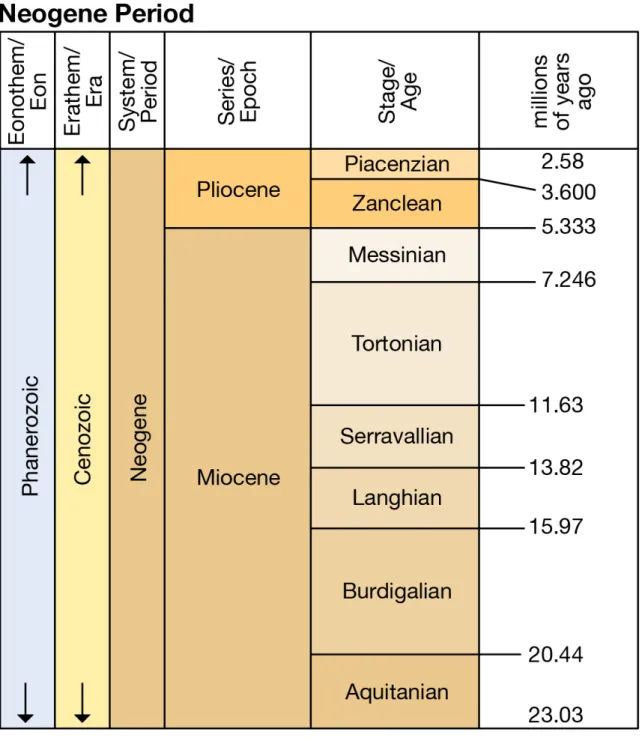
Pliocene (3.6 - 2.58 Ma) is indeed the most recent period of Neogene (Figure1.1). The av-erage temperature of this period is studied to be higher than present level (Haywood and Valdes,2004). The reconstructed CO2concentrations varies from 200ppmv to 450ppmv
and with large uncertainties. For this long interval, the earth system presented relatively stable and warm conditions from 3.6 Ma - 3.0 Ma but also included several cooling per-turbations. Following this period, the earth system entered to a shift stage highlighted by an increasing trend of positive benthic foraminiferal δ18O (Lisiecki and Raymo,2005), de-creasing trends of CO2(e.g.Bartoli et al.,2011;Martínez-Botí et al.,2015;Seki et al.,2010)
as well as sea surface temperatures (e.g.Lawrence et al.,2009). The large intensification of ice sheet in both Hemisphere likely took place around 2.7 Ma indicated by the appear-ance of remarkable IRD ((Flesche Kleiven et al.,2002, and references therein) and large sea-level estimate (e.g. Miller et al., 2012) (Figure1.2). The earth climate then stepped into a cyclic glacial-interglacial state with a 41-kyrs periodicity. Based on the numerous efforts of proxy data and modeling tools, the climate evolution of late Pliocene provides us a good history to study how the climate system function under both warm and cold conditions and also helps to understand the climate sensitivity to a near-present pCO2in
thesis work and will be introduced in the subsection as following.
1.1.1 Mid-Piacenzian warm period
The mid-Piacenzian warm period (MPWP or mid-Pliocene warm period) represents an interval of warm and relatively stable climate between 3.264 and 3.025Ma (Dowsett et al.,2009; Haywood et al., 2010). During this warm phase, the pCO2 records are
esti-mated 50-150ppmv higher than pre-industrial level (280ppmv), the global annual mean temperature may have increased by more than 3 ◦C (e.g. Haywood and Valdes, 2004).
The global extent of arid deserts decreased, and forests replaced tundra in the North-ern Hemisphere high latitudes (Salzmann et al.,2008).The East Asian Summer Monsoon, as well as other monsoon systems, may have been enhanced (Zhang et al., 2013). Ice sheet of both hemispheres may have been largely retreated indicated by increased nega-tive bethic foraminiferal δ18O (Naish and Wilson,2009) and other modeling studies(Lunt et al.,2008)(Hill,2009)(Pollard and DeConto,2009)(Dolan et al.,2015a). The sea-level is estimated to have been 22(+-10m) higher than modern(Miller et al.,2012). Sea surface temperatures (SSTs) were warmer than present level, especially in the higher latitudes and upwelling zones (Dekens et al.,2007;Dowsett et al.,2012). Accordingly,sea ice cover in the high latitudes is studied to be largely decreased, especially during warm seasons (Howell et al.,2016). During this period, the meridional SST gradients is largely decreased as the amplified warming in the high latitudes. The zonal SST gradients is much weaker than present day as the ocean warm pool extended over most of the tropics (Brierley et al.,2009). Thanks to the abundance of proxy data, the MPWP has become a focus for data/model comparisons that attempt to analyze the ability of climate models to repro-duce a warm climate state in earth history.Furthermore, the MPWP has been proposed as an important interval to assess the sensitivity of climate to near-current concentrations of carbon dioxide (CO2) in the long term (hundreds to thousands of years;(Lunt et al.,
2010)). The Pliocene Model Intercomparison Project (PlioMIP) is a co-ordinated inter-national climate modelling initiative to study and understand climate and environments of the Late Pliocene (MPWP), and their potential relevance in the context of future cli-mate change. The first phase of PlioMIP (2008-2014) contributed a lot on modeling the climatic features of the MPWP by several groups of GCMs. However, nearly all models’ results failed to simulate the amplified warming in the high latitudes. Now the on-going
PlioMIP second phase provides a new boundary conditions and focuses on a specific in-terglacial period (MIS KM5c, 3.205Ma) to improve the data-model comparison.
1.1.2 Glacial event of MIS M2
Just before the mid Piacenzian warm period, there was an interval with large excur-sion of δ18O from benthic foraminifera (Lisiecki and Raymo, 2005) which indicating a large cooling state of the earth. This cooling interval is named as Marine isotope stage M2 (MIS M2). MIS M2 is thought to be a glacial comparable period associated with a huge but uncertain sea-level records of 20-60 m below the present level ((Naish and Wilson, 2009); 15 (+-5m); (Miller et al.,2012); 40 (+-10 m);(Dwyer and Chandler,2008); 65m (+-15–25 m ). Direct and indirect proxy data indicate that the expansion of ice sheet during MIS M2 reside in Greenland and Svalbard/Barents Sea (Flesche Kleiven et al.,2002)(Knies et al.,2009)(Moran et al.,2006)(Sarnthein et al.,2009a) ,Iceland(Áslaug Geirsdóttir,2011), Alaska, Canadian Rocky Mountain (Barendregt and Duk-Rodkin,2011), and Antarctic re-gion (Naish and Wilson,2009)(Passchier,2011). Atmospheric CO2values, varying among
different reconstructed methods, were estimated to be within 220-390 ppmv. Each record has large uncertainty of 50 ppmv (Pagani et al., 2010)(Seki et al., 2010)(Bartoli et al., 2011)(Martínez-Botí et al.,2015). Unlike the well-known MPWP (mid-Pliocene warm pe-riod: 3.29 Ma - 2.97 Ma), M2 event is poorly known and remains an enigma in terms of possible scenarios for glaciation. The situation of M2 is relatively different from the Qua-ternary glacial periods in the following aspects: M2 took place during an interval of long warm stable periods; Atmospheric CO2 concentration during M2 was relatively higher
than the Quaternary glaciation period. Besides, reconstructed sea surface temperature in North Atlantic shows a relatively warm condition during M2. All these evidences sug-gest that the M2 event does not occur in typical glacial climate conditions. To explain this anomalous glaciation, geological forcing of brief shallow Panama reopening has been proposed by a recent study (De Schepper et al.,2013). By studying geochemical and pa-lynological marine records from the Caribbean to the North Atlantic, they observed a de-cline in the strength of the North Atlantic current simultaneously to the existence of a Pacific-to-Atlantic through-flow via Central American Seaway (CAS)during this period. Upon that, this cold and fresh through-flow modulated the oceanic circulation and the related heat transport which help to favor the large ice sheet formation. Inversely, the
built-up of the large extent ice sheet could abase the global sea level and then close the shallow opening CAS.The closure of the CAS then brought about an opposite impact on the oceanic circulation and heat transport which help to melt the ice sheet then provide a way-out for M2 glaciation. However, this beautiful assumption has not yet been tested and the dominant factor for M2 glaciation still need to be surveyed.
1.1.3 Plio-Pleistocene Transition
After the MIS M2 glaciation, the earth kept in warming and stable conditions until the beginning of the major climate shift during the Pliocene Pleistocene transition from 3.2-3.0 Ma to 2.5 Ma. During this transition, the sea surface temperature(e.g.Lawrence et al., 2009) and the reconstructed CO2concentrations represent a slowly declining trend.Inversely,
the ice sheet volume in both hemisphere progressively increased and got large expansion around 2.7 Main which can be highlighted by the benthic foraminiferal δ18O (Lisiecki and Raymo,2005)(Maslin et al.,1998)(Mudelsee and Raymo,2005) and marine sedimentary records of ice rafted debris (IRDs) ((Bailey et al., 2013) and reference therein).This tran-sition interval represent an important history of earth climatic system. A lot of studies have been contributed to seek the determinate factors and to understand the underlined mechanisms for the intensification of NHG during this period. These include studies link-ing to the tectonic events which help to modulate both atmospheric and oceanic circu-lation, the most popluar ideas focus on the uplift and erosion of the Tibetan-Himalayan plateau (Ruddiman et al.,1988)(Raymo,1991), the deepening of the Bering Straits and/or the Greenland Scotland ridge (Wright and Miller,1996), the restriction of the Indonesian seaway (Cane and Molnar,2001), and the emergence of the Panama Isthmus (e.g.Haug and Tiedemann,1998;KEIGWIN,1982). However,these tectonic factors are proved by the modelling studies to be helpful but cannot be the major trigger for the large intensifica-tion of NHG (Lunt et al.,2008)(Brierley and Fedorov,2016).Moreover, the timings for the tectonic phases have large uncertainties and are difficult to be constrained. Apart from the tectonic ideas, the role of decreasing CO2 is the recently most approval factor. Lunt
et al.(2008) highlighted the important role of large lowering of pCO2 for the Greenland
glaciation during the late Pliocene. However,Contoux et al.(2015a) based on their recent study prove that the Greenland glaciation might happen with a cumulative process dur-ing a long-term period rather than a rapid build-up. The evolution of Greenland ice sheet
is still unknown due to the paucity of geological data and its light signal in the estimated global sea-level changes. A transient simulation for the Greenland ice sheet evolution may provide an optimal way to resolve this puzzle.
Figure 1.1 – The Neogene Period and its subdivisions.Figure after from 2015 International Com-mission on Stratigraphy (ICS)
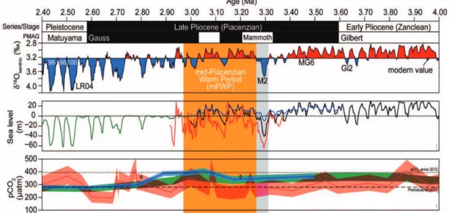
440 460 480 500 520 2.6 3 3.4 3.8 4.2 2400 2600 2800 3000 3200 3400 3600 0 1000 2000 3000 4000 5000 6000 907 644 1307 611 610 984 150 200 250 300 350 400 450 500 2400 2600 2800 3000 3200 3400 3600 Bartoli et al.2011 Stap et al.2016 Martinez et al.2015 Badger et al.2013 Bartoli et al.2011 Van de Wal et al.2011 Seki et al.2010 (Alkenone) Seki et al.2010 (G.ruber)
Piacenzian
Kyrs ago Kyrs ago M2 KM5 98 96 100 G4 G6 Ben th ic d e lta O18 65N Ju ly i n s o la ti o n IR D rec o rd s p CO2 d a ta iNHGFigure 1.2 – A synthesis of Late Pliocene evolution. (a) LR04 benthic isotope stack (Lisiecki and
Raymo,2005); (b) July insolation at 65N (Laskar et al.,2004); (c) Ice rafted detritus (IRD) records
from different studies (DSDP Site 610 (Flesche Kleiven et al.,2002), DSDP Site 611 (Bailey et al.,
2013), ODP Site 644 (Jansen and Sjøholm,1991), ODP Site 907 (Jansen et al., 2000), ODP Site
984 (Bartoli et al.,2011) and site U1307 (Sarnthein et al.,2009a); (d) Reconstructed pCO2records
and model inverse data from different studies (Seki et al.,2010)(Bartoli et al.,2011) (Badger et al., 2013)(Martínez-Botí et al.,2015)(Van De Wal et al.,2011)(Stap et al.,2017)
1.2
Climate forcings and climate modeling
1.2.1 Climate forcings
The climate system is an interactive system consisting of five major components: the atmosphere, the hydrosphere, the cryosphere, the land surface and the biosphere (IPCC). This system is driven and affected by various forcing mechanisms which can be cate-gorized into natural and anthropogenic factors. The natural forcings include the sun’s energy output, change of orbital parameters and large volcanic eruptions which thrown great number of gases and dust particles in the atmosphere. Forcings due to human activ-ities contains increased greenhouse gas concentrations produced by fossil fuel burning, aerosols,and changes in land use surface properties among other things. The imbalance of the incoming and outcoming energy at the top of the atmosphere, defined as "radia-tive forcing" by IPCC report, which is influenced by changes in individual forcing factors, drive directly the climate change.
In this study, two major forcing factors : orbital parameters and CO2concentrations
are presented in the Figure1.2b,d. The orbital parameters are calculated based on the model ofLaskar et al.(2004), which is relatively accurate. However, the CO2
concentra-tions reconstructed based on different proxy data during the late Pliocene are highly un-certain. More studies are still urgently needed to constrain these uncertainties to provide more reliable deep paleoclimate modeling.
1.2.2 Climate modeling
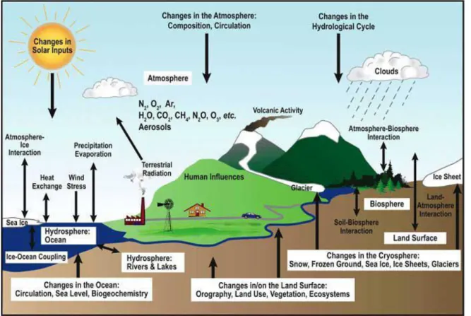
It is largely accepted that the numerical modeling provide us the most effective way to represent paleoclimate and to predict the climate changes in the future. The key concep-tion of any climate model is to represent processes that affect climate.A schematic of the processes that affected the climate system is shown in Figure1.3.The differences among climate models are generally from the extent of simplification in the processes, the res-olution in time and space.Earth system models are currently the most comprehensive tools available for simulating past and future response of the climate system to external forcing, in which biogeochemical feedbacks play an important role.Atmosphere–Ocean General Circulation Models (AOGCMs) are the standard climate models in which the pri-mary function is to understand the dynamics of the physical components of the climate
Figure 1.3 – Shematic for the processes that affected the climate in the earth system model.Figure modified from (Treut et al.,2007)
system (atmosphere, ocean, land and sea ice), and for making projections based on future greenhouse gas (GHG) and aerosol forcing. These models continue to be extensively used, and in particular are run (sometimes at higher resolution) for seasonal to decadal cli-mate prediction applications in which biogeochemical feedbacks are not critical (Source: WG1AR5,Chapter09). In this study, we applied AOGCM of IPSL to accomplish all our nu-merical experiments. The details of this model will be introduced in Chapter 2
However, most existed climate models do not include the cryosphere component of climate system, since large ice sheets and caps require thousands of years to reach equi-librium state. Ice sheet models are generally designed to represent the dynamical and physical processes of ice sheets and ice shelves with different simplified and parameter-ized schemes. Although the ice sheet models have different complexities ,they are gener-ally able to simulate the evolution of the ice over periods on an order of hundred thou-sand or a million year. However, due to the different timescale of functions, it is difficult to achieve a long-term coupled simulation GCM-ISM based on present computational technology. In my thesis, I used GRISLI model (Ritz et al., 2001) to do all the ice sheet modeling work. Moreover, as a part of my thesis work, I introduce a new methodology to
realize a long-term climate transient simulation for Greenland ice sheet during the Plio-Pleistocene transition, which will be introduced in Chapter 5 of this thesis.
1.3 Objectives and scientific issues in the thesis
As we know, the present projection of future climate are based on the understand-ing of the short-term impacts of the variations of the climate forcunderstand-ing in near-present era on climate, which is limited to provide a comprehensive understanding of the climate evolution. Therefore, paleoclimate provides a good means for us to better understand the mechanisms of on-going climate changes. This is why more and more climate models and modelers join in "paleoclimate modeling intercomparison programs (PMIP)", which aims to understand the mechanisms of long-term climate changes, to identify the different cli-matic factors that shape our environment and evaluate the capability of state-of-the-art models to reproduce different climates. The most recent phase of PMIP contains several specific paleoclimate periods like Mid-Holocene ( 6Ka), Last Glacial Maximum ( 21Ka), Last Millennium,Last interglacial (128Ka) and mid Pliocene warm Period ( 3.3-3.0Ma). Among these paleo histories, mid Pliocene warm period is the most suitable interval to study the climate warming under a present-like pCO2 and insolation as introduced in
the section1.1.1. My thesis project started initially in the framework of the PlioMIP and now is already in the second phase as "PlioMIP phase 2". Thus one of my thesis goals is to complete core experiments required by PlioMIP phase 2 and to evaluate the ability of IPSL AOGCM in producing warming climate through the comparison with data and other models’ outputs.
In addition to the study of this warm period of Late Pliocene, we also focus on the change of climate variability along Late Pliocene like the abrupt glacial event MIS M2 prior to MPWP; the progressively intensification of northern hemisphere glaciation during the Plio-Pleistocene.These intervals are of great interest for us to study the mechanisms of the climate change during cooling phases being different from the glaical-interglacial cycles of the late Pleistocene and to understand the interactions among atmospheric , oceanic and cryospheric and vegetation system during a long-term transition. Centered on these targets, three different parts of study have been carried out and will be introduced in this thesis with the order as follows:
1. The mechanism to explain the occurrence and termination of MIS M2 glacial event. 2. The Greenland ice sheet evolution during the Plio-Pleistocene
3. The Earth climatic features under mid-Piacezian warm Period.
Through these three objectives, we aims to address the major scientific questions as following:
1. What could have caused the MIS M2 glacial event and what was it like ?
2. What is the importance of palaeogeography in model simulations of global and re-gional climate change?
3. How was the Greenland ice sheet evolution during the PPT and how critical is at-mospheric CO2concentration pathways to the Greenland ice sheet inception ?
Description of the climate model used in
this study
Contents
2.1 Atmosphere-Ocean Global Circulation Model (AOGCM) . . . 14
2.1.1 Atmosphere and Land . . . 15
2.1.2 Ocean and sea ice . . . 16
2.1.3 New AOGCM version :IPSL-CM5A2 . . . 17
2.1 Atmosphere-Ocean Global Circulation Model (AOGCM)
A very important issue in this thesis is that we perform our simulations with the same models that are currently used for Quaternary PMIP (6ka, 21ka) (Braconnot et al.,2007; Kageyama et al.,2013) and also for CMIP (Dufresne et al.,2013) future climate scenarios, as described in IPCC AR5. Therefore, from the modeling point of view, we may consider that our study is an important sensitivity test to understand how standard IPSL models respond to a slightly different tectonics context. In contrast, a major difference with mod-eling the last glacial-interglacial cycles of the Quaternary or future climates is the uncer-tainty on atmospheric CO2 reconstructions. Indeed, Antarctica ice sheet records describe very well the greenhouse gases content for the last 800 ka (Petit et al.,1999)(EPICA com-munity members, 2004). For Pliocene periods, only indirect proxy reconstructions are available. Although they depict similar tendencies, the absolute values of reconstructed pC02 are different. Moreover, even if plate tectonics did not change drastically during these last three million years, recent orogenesis and seaways closing or opening (central American seaway, Indonesian through-flow) may impact atmospheric and oceanic cir-culation. These changes will drive climate and cryosphere evolutions. In the next three chapters, we will focus on three key periods of this evolution in different contexts.
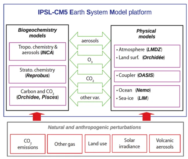
To accomplish the modeling work, we employed two versions of Institut Pierre-Simon Laplace (IPSL) coupled atmosphere-ocean general circulation model (AOGCM):IPSL-CM5A and IPSL-CM5A2.1. IPSL-CM5A is a high resolution coupling model which has been ap-plied in CMIP5 for historical and future simulations (Dufresne et al.,2013) as well as for Quaternary and Pliocene paleoclimatic studies (Contoux et al., 2012; Kageyama et al., 2013). The version of IPSL-CM5A2.1 is designed based on IPSL-CM5A with mainly tun-ning the cloud radiative effect to avoid the global cold bias in the model (Sepulchre et al.,2018 In prep). Moreover, the computational performance of IPSL-CM5A2.1 is improved by about 6 times ( 50 yrs/d) than that of IPSL-CM5A. We will shortly present the informa-tion of each components of the AOGCM as following.Figure2.1show a shematic of IPSL earth system model. In our study, the Bio-geochemistry processes are not activated. More details can be referred (Dufresne et al.,2013).
Figure 2.1 – Shematic for IPSL-CM5 earth system model.Figure after (Dufresne et al.,2013)
2.1.1 Atmosphere and Land
The atmosphere component of IPSL-CM5A is LMDZ model(Hourdin et al.,2013,2006) developed at Laboratoire de Météorologie Dynamique in France. This is a complex model that incorporates many processes decomposed into a dynamic part, calculating the nu-merical solutions of general equations of atmospheric dynamics, and a physical part, calculating the details of the climate in each grid point and containing parameteriza-tions processes such as the effects of clouds, convection, orography (LMD_Modelling_-Team, 2014). Atmosphere dynamics are represented by a finite-difference discretisation of the primitive equations of meteorology (e.g.Sadourny and Laval,1984) on a longitude-latitude Arakawa C-grid(e.g.Kasahara,1977). The chosen resolution of the model is 96x95x39, corresponding to an interval of 3.75 degrees in longitude and 1.9 degrees in latitude. There are 39 vertical levels, with around 15 levels above 20 km. This model has the specificity to be zoomed (the Z of LMDZ) if necessary on a specific region and then may be used for
regional studies (e.g.Jost et al.,2009).
The land component in IPSL-CM5A is ORCHIDEE (Organizing Carbon and Hydrology In Dynamic Ecosystems, (Krinner et al.,2005)) is composed of three modules: hydrology, carbon cycle and vegetation dynamics. The hydrological module, SECHIBA (Ducoudré et al.,1993), describes exchange of energy and water between atmosphere and biosphere, and the soil water budget(Krinner et al., 2005). The river routing scheme combines the river flow with a cascade of three reservoirs: the stream and two soil reservoirs with dif-ferent time constants (Marti et al., 2010). Vegetation dynamics parametrisation is derived from the dynamic global vegetation model LPJ (Krinner et al., 2005; Sitch et al., 2003). The carbon cycle model simulates phenology and carbon dynamics of the terrestrial bio-sphere (Krinner et al., 2005). Vegetation distributions are described using 13 plant func-tional types (PFTs) including agricultural C3 and C4 plants, which are not used in the mPWP simulations, bringing down the number of PFTs to 11, including bare soil. In our case, hydrology and carbon modules are activated, but vegetation is prescribed as the same withContoux et al.(2012), using 11 PFTs, derived from the PRISM3 vegetation dataset (Salzmann et al., 2008). Therefore, soil, litter, and vegetation carbon pools (in-cluding leaf mass and thus LAI) are calculated as a function of dynamic carbon allocation (Krinner et al., 2005).
2.1.2 Ocean and sea ice
The ocean model is NEMOv3.2 (Madec, 2008) which includes three principle mod-ules: OPA (for the dynamics of the ocean), PISCES (for ocean biochemistry), and LIM (for sea ice dynamics and thermody- namics). The configuration of this model is ORCA2.3 (Madec and Imbard,1996), which uses a tri-polar global grid and its associated physics. There are 31 unequally spaced vertical levels and a nominal resolution of 2◦that is refined
up to 0.5◦in the equatorial area.Temperature and salinity advection is calculated by a
to-tal variance dissipation scheme (Lévy et al.,2001)(Cravatte et al.,2007). The mixed layer dynamics is parameterized using the Turbulent Kinetic Energy (TKE) closure scheme of Blanke and Delecluse (1993) improved by Madec (2008). The sea ice module LIM2 is a two-level thermodynamic-dynamic sea ice model (Fichefet and Morales Maqueda 1997, 1999). Sensible heat storage and vertical heat conduction within snow and ice are deter-mined by a three-layer model. OASIS model plays as a coupler (Valcke,2006) to
interpo-late and exchange the variables and to synchronize the models. This coupling and inter-polation procedures ensure local energy and water conservation (Dufresne et al.,2013).
Ice-Shelf Ice-Shelf Sea level
Accumulation
Flow
T S = -50°C Geothermic Flux Geothermic Flux MeltingTemperatures
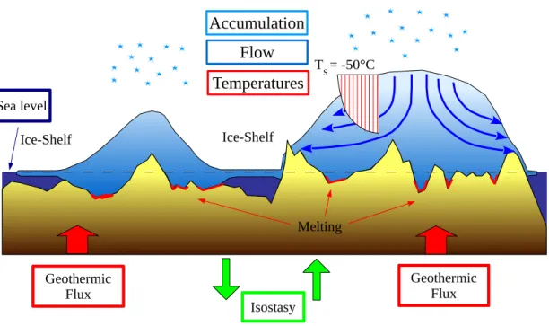
IsostasyFigure 2.2 – Schematic design for GRISLI ice sheet model. Modified after Dumas (2002).
2.1.3 New AOGCM version :IPSL-CM5A2
IPSL-CM5A2 (for which a detailed description can be found in Sepulchre et al., in prep.) is an updated version of the CMIP5 IPSL-CM5A2 earth system model (ESM). The basics (LMDZ5A physics schemes, ORCHIDEE 2-level hydrology) and the resolutions of each components have been kept identical. However critical changes between the two ESMs include (i) technical developments to make IPSL-CM5A2 run faster, (ii) updates of different components and (iii) a retuning to correct IPSL-CM5A cold bias. On the tech-nical side, IPSL-CM5A2 benefits from hybrid parallelization combining MPI paralleliza-tion on latitudinal bands for LMDZ-ORCHIDEE and shared memory parallel processing (OpenMP) on vertical levels, allowing the model to be run on more than 300 cores. Com-putation time has thus improved, switching from 8yrs per day in IPSL-CM5A to up to 62yrs perday in IPSL-CM5A2.
compartment. NEMO v3.6 has been included in the model, with the vertical levels now discretized using the “partial steps“ scheme. ORCHIDEE has benefited from numerous bug corrections, especially on continental water fluxes, which conservation is now guar-anteed. LMDz is rather similar to IPSL-CM5A version, modulo minor bug corrections. Re-tuning of the model has been done by altering the cloud radiative effect. The des-ignated target was a pre-industrial temperature approaching 13.5◦C with a null surface
energy balance. Latest multi-millenia experiments with IPSL-CM5A2 provided a global 2-m temperature of 13.25◦C, a value that Sepulchre et al. considered acceptable. Known
biases of IPSL-CM5A-LR were not corrected: they include a double ITCZ structure over the Pacific ocean, underestimated precipitation over the Amazonian basin and the lack of deepwater formation in the Labrador sea. Still, tuning towards warmer temperatures improved the overall Atlantic Meridional Overturning Circulation by 2-3 Sv.
2.2 Ice sheet model
The ice sheet model used in this study is the GRenoble Ice-Shelf and Land-Ice model (GRISLI). GRISLI is a three-dimensional thermo-mechanical model that simulates the evolution of ice sheet geometry (extension and thickness) and the coupled temperature–velocity fields in response to climate forcing. A comprehensive description of the model can be found inRitz et al.(2001) and (Peyaud et al.,2007). Figure2.2represents a schematic de-sign for the GRISLI ice sheet model. Over the grounded part of the ice sheet, the ice flow resulting from internal deformation is governed by the shallow-ice approximation ( Mor-land,1984). The model also deals with ice flow through ice shelves using the shallow-shelf approximation (MacAyeal,1989) and predict the large-scale characteristics of ice streams using criteria based on the effective pressure and hydraulic load. At each time step, the velocity and vertical profiles of temperature in the ice are computed as well as the new geometry of the ice sheet. The isostatic adjustment of bedrock in response to ice load is governed by the flow of the asthenosphere, with a characteristic time constant of 3000 years, and by the rigidity of the lithosphere. The temperature field is computed both in the ice and in the bedrock by solving a time-dependent heat equation.The surface mass balance is defined as the sum between accumulation and ablation computed by the pos-itive degree-day (PDD) method (Fausto et al.,2009).In this study, we use GRISLI on three different grids. Two 40km grids : one is for the Northern Hemisphere (Hereafter
"GRISLI-Table 2.1 – Major parameters applied in the GRISLI model
Basal drag coefficient 1500 m yr/Pa
Topographic lapse rate, annual 6.0 °C/km
Precipitation ratio parameter 0.07/°C
PDD standard deviation of daily temperature 5.0 °C
PDD ice ablation coefficient 8.0 mm/day°C
PDD snow ablation coefficient 5.0 mm/day°C
NH"), second is for Antarctica. Another refined cartesian grid (15kmx15km) was used on Greenland (Hereafter "GRISLI-Greenland").Table2.1show the standard parameters ap-plied in the GRISLI model.
Exploring the MIS M2 glaciation under a
warm and high CO2 Pliocene climate
Contents
3.1 Introduction . . . 22
3.2 The issue on Central American Seaway hypothesis . . . 25
3.2.1 The classical CAS hypothesis . . . 25
3.2.2 The “shallow re-opening CAS” hypothesis for MIS M2 glaciation . . 28
3.2.3 Sensitivity experiment with shallow opening CAS . . . 30
3.3 Paper published in Earth Planetary Science Letters "Exploring the MIS M2 glaciation occurring during a warm and high atmosphere CO2 Pliocene
background climate" . . . 32
3.1 Introduction
Prior to the perennial Greenland glaciation around 2.7 Ma, a large glaciation MIS M2 (3.312 – 3.264 Ma) took place locating in the interval between two warm periods. The estimated sea-level drops during this glaciation have large uncertainties and vary from 20 meters to 60 meters ((Dwyer and Chandler,2009; Miller et al., 2012; Naish and Wil-son,2009), Figure3.3), which associated with likely large expanded land ice in both hemi-spheres ((De Schepper et al.,2014),Figure3.2). Moreover, the reconstructed pCO2 records during this event with the range of 220 - 405 ppmv(Bartoli et al.,2011;Martínez-Botí et al., 2015;Pagani et al.,2010;Seki et al.,2010) are much higher than that during Quaternary glaciation (Figure3.1). Unlike the mid Pliocene warm episode from 3.3 to 3.0 Myr ago, which is well documented from marine data (Dowsett et al., 2012), continental records (Salzmann et al.,2008) and model studies (Haywood et al.,2016), MIS M2 is poorly under-stood and there are few modeling studies focusing on the MIS M2 glaciation termination and decay. Only one recent work byDolan et al.(2015b) studied M2 glaciations with dis-cussing the likely extent of ice sheets during M2 glaciation by confronting the simulated climate conditions with different land ice scenarios to the available proxy data. Their study demonstrated the possibility of the existence of a larger-than-modern ice sheet dur-ing M2, but the drivdur-ing factors were not discussed. The mechanism for M2 onset and de-cay remains still an enigma. Regarding the speculative features of M2, the classical forcing factors may not be enough to explain. Nevertheless, a recent geological hypothesis based on the marine proxy data invoked the specific role of re-opening and closing of shallow Central American Seaway (CAS) to explain the triggering and decay of M2 glaciation (de-tails are represented in Section3.2.2. However, this hypothesis has not been validated by modeling studies. Therefore, in this study, we aim at exploring the mechanisms un-derlying M2 formation and termination. For this purpose, we firstly test this reasonable geological hypothesis,secondly discuss the roles of classical forcing factors and internal feedbacks and thirdly quantify the M2 glaciation extent with all favorable forcing factors. Since this work has been already published, A completed story about this work can be found in my paper included in Section3.3. Before going to the paper, I will give a brief review on the Central American Seaway issues in Section3.2.2.
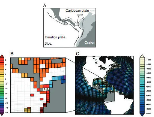
Figure 3.1 – Marine isotope stage M2 in the long-term climate evolution of the Pliocene. Figure modified from De Schepper et al.,2013
Figure 3.2 – The distribution of ice sheets at around 3.3Ma based on the marine and terrestrial records. Figure modified from De Schepper et al.,2014
3.2 The issue on Central American Seaway hypothesis
3.2.1 The classical CAS hypothesis
Under modern conditions, sea waters represent strong contrast in sea surface temper-ature (SST) and salinity (SAL) between East Pacific and Caribbean sea (Figure3.3). How-ever, these two sea waters deeply connected before the formation of the long peninsula connecting Panama to North America. Since the Early Miocene (ca.23–17 Ma), the Central American Seaway (CAS) constricted to a narrow range of 200 km (Montes et al.,2012a,2012b). Afterwards the marked uplift of the sill underwent and shut off deep-water flow across the isthmus between 12 to 10 Ma (Duque-Caro,1990). However, the shallow water exchange continued via CAS until the late Pliocene ((Molnar,2008) and reference therein). While the actual timing of the final closure of the CAS is largely debated, studies based on bio-geographical and paleoceanographical data have proved the early Pliocene to be the ma-jor period where underwent the progressively shoaling of the CAS (KEIGWIN,1982)(Haug and Tiedemann,1998).
Therefore, regarding the Pliocene period, one question of the particular interest is the closure or shoaling of the CAS. The impact of closure of the CAS on the high latitude cli-mate has been extensively studied and remains largely debated. Theoretically, the closure or restriction of the CAS resulting in a cessation of fresher water transport from Pacific to the Caribbean sea, could affect the climate by enhancing the Atlantic meridional over-turning circulation (AMOC) and modifying the heat and moisture transport. The classical ‘Panama Hypothesis’, first proposed by Keigwin(1982), stated that one of the effects of this change is to enhance evaporation rates in the North Atlantic, providing an enhanced moisture flux to northern high latitudes, increased precipitation and help to the inception or intensification of NHG beginning at 3 Ma (Haug and Tiedemann,1998)
Numerous modeling studies have conducted to investigate the potential effects of the CAS closure or shoaling on the climate (Maier-Reimer et al. 1990; Mikolajewicz et al. 1993; Mikolajewicz and Crowley et al.,1997;Murdock et al. 1997; Nisancioglu et al. 2003; Prange and Schulz 2004; Klocker et al. 2005; von der Heydt and Dijkstra 2005; Schneider and Schmittner 2006;Brierley and Fedorov, 2016 and reference therein). Most of these stud-ies demonstrate the role of the CAS closure in enhancing Atlantic thermohaline circula-tion associated with a strengthened North Atlantic Deep Water (NADW) formacircula-tion
result-ing from the decreased fresher water transport from the Pacific into Atlantic, while few of these studies demonstrate the important role of CAS in the NHG reinforcement. As discussed before, the enhanced northward moisture transport that may help to increase NHG intensification (iNHG) is accompanied with the enhanced heat transport associ-ated with the shoaling or closure of the CAS, which likely help to delay the iNHG. But the relative contributions of these two effects of the closure CAS is actually not very clear. Klocker et al.,(2005) demonstrate that the perennial snow cover decreased after the clo-sure of the CAS, implying the doubtful role of the cloclo-sure of CAS in the iNHG. Lunt et al., (2008) demonstrated that the closure of the CAS contributes little to the formation of the land ice in Greenland. Moreover, Brierley and Fedorov et al., 2016 compared three possi-ble seaway changes during the Pliocene and demonstrated that both two tropical seaways (CAS and Indonesia Seaway) play much weaker roles in the high latitude climate than the high latitude seaway of Bering strait.
Salinity Temperature
Figure 3.3 – Sea surface salinity and temperature distribution in the tropical eastern Pacific region
~3.315 Ma ~3.285 Ma
Shallow opening Panama Seaway during interglacial MG1
Southward shift of the NAC , reduction of northward heat transport, the inception of ice sheets
Closure of the shallow Panama seaway by the lowering of sea level resulting from large extent of ice sheet built-up Rebuilt-up of Caribbean warming pool
after the closure of Panama seaway Re-establishment of northward heat transport via rebuilt-up of normal NAC, the termination of glaciation
Figure 3.4 – The shematic for "shallow opening Panama Seaway" hypothesis. Figure modified from De Schepper et al.,2013
3.2.2 The “shallow re-opening CAS” hypothesis for MIS M2 glaciation
Although restriction of surface waters through the Central American Seaway might occur during the Early Pliocene (4.5–4.3 Ma) based on planktonic foraminifera data (e.g. Haug and Tiedemann,1998), the final tectonic closure of the Central American Seaway might not occur until 2 Ma (Jackson et al., 1993). During this long interval, the exchange of surface waters was probably constrained up to a 100-meters sill depth and dynam-ically affected by the glacial induced sea-level change (Groeneveld et al., 2014). Even such shallow water exchange might have had influenced the Northern Hemisphere cli-mate. A study of De Schepper et al. (2013) put forward the hypothesis that a re-opening and closing of the shallow CAS may have triggered the onset and the termination of the M2 glaciation. This hypothesis provides for the first time an explanation for the forma-tion and decay of the NH ice sheets during M2 in relaforma-tion to tectonic and glacio-eustatic change. Based on dinoflagellate cysts and geochemical proxy data from different Ocean
Figure 3.5 – The position of narrow Central American seaway since the early Miocene (a) and the related CAS location in the model (b and c). Figure modified from Sepulchre et al.,2014
Drilling Project sites, they conjecture that a re-opening of the shallow CAS occurring be-fore and during the M2 event allowed seawaters flowing from the Pacific to the Atlantic. The fresher and cold inflow seawater helped to weaken the North Atlantic circulation and to cool the northern high latitudes. Then the cooling was gradually amplified by the pos-itive sea ice albedo feedback, the adaptation of vegetation to colder climates and pCO2 changes, finally leading to substantial ice sheet growth in NH high latitudes (De Schepper et al., 2013). Inversely, the large ice volume accumulated over land would then produce a sea-level drop large enough to close the CAS. Following this glacio-eustatic closure, the ocean circulation shifted to its modern state and warmed the northern high latitudes, trig-gering the deglaciation. This hypothesis has gained a lot of attention because it provides an explanation both for the onset and the termination of the M2 glaciation. Moreover, this seaway hypothesis would better fit the short duration of the M2 glaciation comparing to other long-term geological processes and the glacio-eustatic closure corresponds well to the sea-level drop estimates (20–60 m)(Figure3.4). However, this hypothesis is
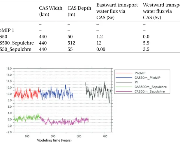
funda-Table 3.1 – Results of the CAS opening in the model CAS Width (km) CAS Depth (m) Eastward transport water flux via CAS (Sv)
Westward transport water flux via CAS (Sv) AMOC (Sv) PI – – – – 11.4 PlioMIP 1 – – – – 11.7 CAS50 440 50 1.2 0.0 11.5 CAS500_Sepulchre 440 512 12 5.9 3.9 CAS50_Sepulchre 440 55 0.09 3.5 2.5
Modeling time (years)
Figure 3.6 – Evolutions of AMOC index during the modeling time in each simulation that
intro-duced in the table3.1
mentally different from the classical CAS hypothesis and it has not yet been tested. Thus in this study, we provide the first modeling effort to validate this assumption.
3.2.3 Sensitivity experiment with shallow opening CAS
The set-up of shallow opening CAS in the model
As discussed in the above, Montes et al. (2012a, 2012b) suggest that the CAS constriced to a narrow range of 200km (As showing in Figure3.5a). However, the horizontal resolu-tion in NEMO ocean model is 2 degrees in tropical region (see at chapter2), which means the CAS width only takes up one grid in the model. Regarding the low sensibitlity to this one grid modification in our model, here we modify two grids of our model at 8N asso-ciated with 440km width to represent the narrow CAS and the location is consistent with the previous study of Sepulchre et al.(2014) (Figure3.5). To take into account the glacio-eustatic closure of the CAS after M2, here we set-up a 50m sill depth for this narrow CAS in
the model. The sensitivity experiment with the openning CAS is carried out based on the PlioMIP 1 standard simulation of Contoux et al.,(2012), which show a present-comparable AMOC of ca.11x106m3.s−1(i.e., 11 Sverdrups, hereafter Sv).
The modification on water current after CAS opening
After opening this shallow and narrow CAS, we observed an expected eastward water transport of ca. 1.2 Sv via CAS (from Pacific ocean to Caribbean region ). This fresher water invasion reduces the SAL and SST in the Caribbean sea and further reduces the North At-lantic current. All the effects associated with the opening CAS are in good agreement with data observation (De Schepper et al.2013) except for the magnitude of each influences. More details can be found in section3.3.
Table3.1represents a comparison work between our CAS50 experiment and the CAS simulations of Sepulchre et al.,(2014). However, with a similar sill depth of CAS (50me-ters), Sepulchre et al., (2014) (CAS50_sepulchre) observed an opposite water transport from Caribbean sea to Pacific region . The large difference can be attributed to the dif-ferent initial states of AMOC in our experiment.In a theoretical study of Nof et al. (2003), they have shown how the circulation may change when different seaways are opened and closed, especially Bering straits, Drake passage and Central American seaway In particu-lar, this study demonstrates that the water flow direction via the CAS highly depends on the initial North Atlantic Deep Water (NADW) state, when NADW is strong enough, the invasion of water is from Pacific to Atlantic, otherwise, water current is from Atlantic to Pacific. Accordingly, we find that the initial state of AMOC in CAS50_sepulchre is about 3.9 Sv, which is based on their CAS500 experiment (Figure3.6). Nevertheless, our CAS50 experiment are based on PlioMIP 1 (Contoux et al., 2012), which show a much stronger AMOC (11.7 Sv). This results further demonstrate the sensitivity of the IPSL model to this narrow CAS set-up.
Regarding that our sensitivity experiment of CAS50 is carried out under a high pCO2 condition (405 ppmv), it is also necessary to test the CAS50 effects under a low pCO2 condition. Thus, based on the CAS50 experiment of 405ppmv, we carried out another CAS50 experiment with 280ppmv of pCO2. Then we find that, with a lower pCO2, the water current keep the same direction but get an increased water flux ( 2 Sv).More details are found in the next section.
3.3 Paper published in Earth Planetary Science Letters
"Ex-ploring the MIS M2 glaciation occurring during a warm
and high atmosphere CO2 Pliocene background climate"
Contents lists available atScienceDirect
Earth
and
Planetary
Science
Letters
www.elsevier.com/locate/epsl
Exploring
the
MIS
M2
glaciation
occurring
during
a
warm
and
high
atmospheric
CO
2Pliocene
background
climate
Ning Tana,∗,Gilles Ramsteina,Christophe Dumasa,Camille Contouxb,
Jean-Baptiste Ladanta,Pierre Sepulchrea,Zhongshi Zhangc,d,e,Stijn De Schepperc
aLaboratoiredesSciencesduClimatetdel’Environnement,LSCE/IPSL,CEA-CNRS-UVSQ,UniversitéParis-Saclay,F-91191Gif-sur-Yvette,France bAix-MarseilleUniversité,CNRS,IRD,CollègedeFrance,CEREGEUM34,Europôledel’Arbois,13545Aix-enProvence,France
cUniResearchClimate,BjerknesCentreforClimateResearch,Nygårdsgaten112-114,5008Bergen,Norway dDepartmentofAtmosphereScience,ChinaUniversityofGeoscience,430074,Wuhan,China
eNansen-ZhuInternationalResearchCenter,InstituteofAtmosphericPhysics,ChineseAcademyofSciences,100029,Beijing,China
a r t i c l e i n f o a b s t r a c t
Articlehistory:
Received23July2016
Receivedinrevisedform27April2017 Accepted28April2017
Availableonline25May2017 Editor:M.Frank
Keywords:
glaciation MISM2
CentralAmericanSeaway latePliocene
warmclimate icesheetmodelling
PriortotheNorthernHemisphereglaciationaround∼2.7 Ma,alargeglobalglaciationcorrespondingtoa 20to60 msea-leveldropoccurredduringMarineIsotopeStage(MIS)M2(3.312–3.264 Ma),interrupted theperiodofglobalwarmthandhighCO2concentration(350–450 ppmv)ofthemidPiacenzian.Unlike thelateQuaternaryglaciations,theM2glaciationonlylasted50 kyrsandoccurredunderuncertainCO2 concentration(220–390 ppmv).ThemechanismscausingtheonsetandterminationoftheM2glaciation remainenigmatic, butarecent geologicalhypothesis suggests that there-opening and closingofthe shallowCentralAmericanSeaway(CAS)mighthaveplayedakeyrole.Inthisarticle,thankstoaseries ofclimatesimulationscarriedoutusingafullycoupledAtmosphere OceanGeneral CirculationModel (GCM)andadynamicicesheetmodel,weshowthatre-openingoftheshallowCAShelpsprecondition thelow-latitudeoceaniccirculationandaffectstherelatednorthwardenergytransport,butcannotalone explaintheonset ofthe M2glaciation.The presenceofashallow openCAS,togetherwith favourable orbitalparameters,220 ppmvofCO2concentration,and therelatedvegetationandicesheetfeedback, ledtoaglobalicesheetbuild-upproducingaglobalsea-leveldropinthelowestrangeofproxy-derived estimates.More importantly,our results showthat the simulated closureofthe CAShas anegligible impactontheNHicesheetmeltandcannotexplaintheMISM2termination.
2017ElsevierB.V.Allrightsreserved.
1. Introduction
Despiteabsolutedifferences, mostatmospheric carbondioxide proxiespointtowardsadrasticdecreaseassociatedwithlarge cool-ing fromthe LateEocene to the Quaternary (Pagani et al., 2005; Zachosetal.,2001).ThefirstmajoratmosphericCO2 thresholdfor
ice sheet build-up is reached around 34 Ma, when the Antarc-tic glaciation began under CO2 levels equivalent to about three
timesthoseofthepreindustrial concentrations(DeContoand Pol-lard, 2003; Ladantetal., 2014; Gassonetal., 2014). Theonset of extensiveNorthernHemisphereglaciationoccurredapproximately 30million yearslater around3.0–2.7 Ma(Luntetal., 2008), ulti-matelyleadingto theglacial–interglacialcyclesoftheQuaternary (e.g.GanopolskiandCalov,2011).However,priortothisglaciation, a major ephemeral glacial event took place, the Marine Isotope
* Correspondingauthor.
E-mailaddress:[email protected](N. Tan).
Stage (MIS) M2 (3.312–3.264 Ma), producing a ∼0.5❤ shift of benthic foraminiferal δ18O (Lisiecki and Raymo, 2005). The
sea-level drop produced by thisglacial event has been estimated at 20 to 60 m by different proxy estimates (Dwyer and Chandler, 2009; Miller etal., 2012; NaishandWilson, 2009). As a compar-ison, 20–60 m sea level drop represents between one sixth and nearlyhalfofthesealeveldropduringtheLastGlacialMaximum. Therefore,theM2icesheetswerenot onlyconfinedtoGreenland butmust havespread over the NorthernHemisphere continents. Also,acontributionfromanexpandedAntarcticicesheetsislikely (detailedevidenceforicesheetsduringMISM2aresummarised by DeSchepperetal.,2014).Nevertheless,theM2glaciationhassome very peculiar characteristics with respect to Quaternary glacia-tions:first, thisglacial eventoccurredintheinterval oftwolong andstablewarmperiodsandonlylastedfor∼50 kyr,whichishalf
the duration of recent Quaternary glacial cycles (e.g. Ganopolski and Calov, 2011). In the southern Hemisphere, the East Antarc-ticicesheets were presentandlastedduringthe mid-Piacenzian warm period (Hill et al., 2007), whereas the West Antarctic ice
http://dx.doi.org/10.1016/j.epsl.2017.04.050 0012-821X/2017ElsevierB.V.Allrightsreserved.