HAL Id: tel-02132659
https://tel.archives-ouvertes.fr/tel-02132659
Submitted on 17 May 2019
HAL is a multi-disciplinary open access
archive for the deposit and dissemination of
sci-entific research documents, whether they are
pub-lished or not. The documents may come from
teaching and research institutions in France or
abroad, or from public or private research centers.
L’archive ouverte pluridisciplinaire HAL, est
destinée au dépôt et à la diffusion de documents
scientifiques de niveau recherche, publiés ou non,
émanant des établissements d’enseignement et de
recherche français ou étrangers, des laboratoires
publics ou privés.
Cavity non destructive detection on an optical lattice
clock
Grégoire Vallet
To cite this version:
Grégoire Vallet. Cavity non destructive detection on an optical lattice clock. Astrophysics [astro-ph].
Université Paris sciences et lettres, 2018. English. �NNT : 2018PSLEO026�. �tel-02132659�
Préparée à l’Observatoire de Paris
Détection non destructive en cavité pour une horloge à
réseau optique au strontium.
Soutenue par
Grégoire Vallet
Le 13 décembre 2018
École doctorale n
o564
Physique en Île-de-France
Spécialité
Physique (milieux dilués et
optique)
Composition du jury :
Caroline Champenois
chargée de recherche CNRS,
Aix-Marseille Université rapporteuse
Robin Kaiser
directeur de recherche CNRS, Univer-sité Côte d’Azur
rapporteur
Morgan Mitchell
professeur examinateur
Jakob Reichel
professeur, Sorbonne université examinateur
Sébastien Bize
Chargé de recherche CNRS directeur de thèse
Jérôme Lodewyck
Contents
1 Introduction 5
1.1 Clock operation activities . . . 5
1.2 Systematics investigation and assessment . . . 5
1.3 Non-destructive detection . . . 6
2 Time scales and standards, a historical introduction 7 2.1 Twelve hours in the night . . . 7
2.2 Calendars, time units and time scales. . . 9
2.3 Universal Time . . . 10
2.4 Newtonian and post-Newtonian time scales . . . 11
2.4.1 Coordinates systems in use . . . 11
2.4.2 The Newtonian absolute time scale . . . 11
2.4.3 The Special Relativity time scale . . . 12
2.4.4 General Relativity time scale . . . 12
2.5 Coordinated universal times . . . 12
2.5.1 International time scales in practice . . . 12
2.5.2 Universal time scales and atomic standards . . . 13
2.6 International Atomic Time . . . 13
2.6.1 Relativistic TAI . . . 13
2.7 From a second to an other . . . 14
2.7.1 The ephemeris second . . . 14
2.7.2 The atomic second . . . 14
2.7.3 Discrepancy between the S.I. time unit and the unit of the time scale . . . 14
2.7.4 Towards a new definition . . . 14
I
Clocks and their characterization
17
3 Stability, accuracy and uncertainty 17 3.1 Time or frequency ? . . . 173.2 Mathematical model of oscillator signals . . . 18
3.2.1 Uniqueness of representations and Fourier frequencies . . . 18
3.3 Characterization of oscillators . . . 19
3.3.1 Time-domain frequency stability characterization . . . 20
3.3.2 Frequency-domain frequency stability characterization . . . 21
3.3.3 From frequency-domain to time-domain . . . 22
3.4 Concept of accuracy . . . 22
3.5 Uncertainty . . . 23
4 The SYRTE’s strontium optical lattice clocks. 24 4.1 Basics of atomic clocks . . . 24
4.2 Why a strontium clock? . . . 25
4.2.1 High-Q transitions . . . 26
4.2.2 High number of atoms probed. . . 26
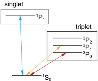
4.2.3 Group II atoms and their singlet-triplet structure. . . 26
4.2.4 Boson or fermion ? . . . 26
4.2.5 Why strontium ? . . . 27
4.3 SYRTE clocks architecture . . . 28
4.3.1 SYRTE optical lattice clocks . . . 28
4.4 SrB clock setup and operation. . . 29
4.4.1 The vacuum system . . . 29
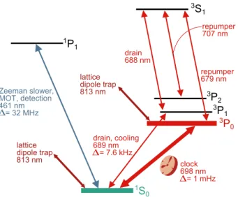
4.4.2 The lasers system. . . 30
4.4.3 The clock sequence . . . 32
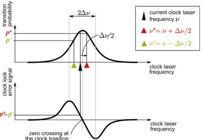
4.4.4 Clock lock. . . 33
4.5 Clock performances. . . 33
4.5.1 State-of-the-art: accuracy . . . 34
4.6 SYRTE strontium clocks uncertainty budget. . . 35
4.6.1 Black-body radiation shift . . . 36
4.6.2 Quadratic Zeeman shift . . . 37
4.6.3 Lattice shifts . . . 38
4.6.4 Density shift . . . 38
4.6.5 Line pulling . . . 38
4.6.6 Background collisions . . . 38
4.6.7 Static charges . . . 38
II
Study of two frequency shift sources: hyperpolarizability and hot
col-lisions
40
5 Hyperpolarizability 40 5.0.1 Why a lattice trap? . . . 405.0.2 Perturbations induced by the trap . . . 42
5.0.3 Classical polarizability and irreducible tensor decomposition. . . 44
5.1 Quantum polarizability . . . 45
5.1.1 Tensor decomposition of the polarizability . . . 46
5.1.2 Polarizability in presence of magnetic field. . . 48
5.1.3 Polarizability measurements . . . 49
5.1.4 Differential measurement and magic wavelength. . . 50
5.2 Hyperpolarizability . . . 51
5.2.1 Tensor decomposition of the hyperpolarizability. . . 52
5.2.2 Hyperpolarizability measurement . . . 54
6 Hot collisions shift 56 6.1 Neutral atoms interaction potential . . . 56
6.2 Hot collisions treatment so far. . . 57
6.2.1 Background gas collisions in micro wave clocks . . . 57
6.2.2 Background gas collisions in optical lattice clocks . . . 57
6.3 Classical preliminaries . . . 57
6.4 Quantum scattering theory in brief . . . 59
6.4.1 Center of mass frame Lipmann-Schwinger equation . . . 59
6.4.2 Asymptotic behavior . . . 59
6.4.3 Differential scattering cross section . . . 59
6.4.4 Partial wave expansion. . . 60
6.5 Frequency shift cross section. . . 62
6.5.1 Master equation . . . 62
6.5.2 Interpretation in term of frequency shift . . . 66
6.6 Quasi-classical regime . . . 67
6.6.1 Quasi-classical momentum and wave functions . . . 67
6.6.2 Quasi-classical phase shift . . . 68
6.7 Losses . . . 69
6.7.1 Losses for an incoming flux of background gas particles . . . 69
6.7.2 Losses for a Maxwell-Boltzmann distribution . . . 69
6.8 Shift and losses . . . 70
6.8.1 Shift and losses, other approach. . . 71
6.9 Hot collisions shifts measurement . . . 71
6.9.1 Hot collision shift model . . . 71
6.9.2 Atoms lifetime in the trap . . . 71
6.9.3 Hot collisions shift measurement . . . 73
6.10 Probing hot collisions shifts: qualitative approach. . . 74
III
Continental scale clock comparison
76
7 International clock comparison 76
7.1 Fiber links comparisons . . . 76
7.1.1 Working principle . . . 76
7.1.2 Measuring frequency ratio from experimentally accessible quantities . . . 80
7.1.3 link stabilization . . . 81
7.1.4 Connection of links. . . 81
7.2 Continental scale comparisons . . . 82
7.2.1 June 2017 comparison campaign . . . 82
7.2.2 Early 2018 comparison campaign . . . 84
7.2.3 Stability of a single clock . . . 86
IV
Pushing forward the stability limits
89
8 Stability limitation and challenges 89 8.1 Dick effect . . . 898.1.1 Dick effect for a Rabi interrogation . . . 89
8.1.2 Ramsey interrogation . . . 92
8.2 Quantum projection noise . . . 93
8.3 Instability contributions hierarchy . . . 94
8.3.1 Expected stability improvements . . . 95
8.3.2 Measurement of detection, clock laser induced and quantum projection noises . . . 96
8.4 Cavity assisted detection as a solution to both limitations . . . 98
9 Trap destruction mechanism 99 9.1 Standard fluorescence detection . . . 99
9.2 Trap destruction by photon scattering . . . 99
9.2.1 Absorption momentum transfer for free atoms. . . 100
9.2.2 Absorption momentum transfer in the Lamb-Dicke regime . . . 101
9.2.3 Emission momentum transfer . . . 101
9.2.4 Heating and loss rates . . . 102
9.3 Conclusion . . . 106
10 Detection systems characterizations 108 10.1 The Hamamatsu 9200 C camera . . . 108
10.1.1 Camera counts calibration . . . 108
10.1.2 Signal to noise ratio analysis . . . 110
10.1.3 Detection noise . . . 112
10.1.4 Applicability to classical non destructive detection. . . 112
10.2 Photo multiplier tube . . . 113
10.2.1 Photo multiplier tube for non destructive detection . . . 113
10.2.2 Counting atoms with the PMT . . . 116
11 Cavity assisted classical non destructive detection (CNDD) 117 11.1 Phase imprint: collinear transport of information . . . 117
11.1.1 Limitation of camera and PMT for CNDD . . . 117
11.1.2 Phase imprinted by the atoms on the probe field . . . 117
11.2 CNDD algebra . . . 120
11.2.1 Generation of the probe sidebands and cavity-atoms response. . . 120
11.2.2 Half round trip phase shift . . . 123
11.2.3 Cavity response. . . 124
11.2.4 PDH-like error signal. . . 124
11.2.5 Atomic signal . . . 124
12 CNDD implementation 128
12.1 Setup . . . 128
12.1.1 The in-vacuum cavity stabilization . . . 128
12.1.2 The probe light . . . 128
12.1.3 Tri-chromatic cavity . . . 130
12.1.4 The PDH-like setup . . . 133
12.1.5 Generation of the signals . . . 134
12.1.6 The probe light sidebands lock to the cavity. . . 134
12.2 System parameters adjustment . . . 134
12.2.1 Adjustment of Ω . . . 134
12.2.2 Choice of β . . . 134
12.2.3 Calibration of β . . . 135
12.2.4 Voltage to phase slope calibration . . . 135
12.3 Noise and SNR analysis . . . 136
12.3.1 residual cavity length fluctuations and EOM modulation induced noise . . . 136
12.3.2 Photodetection noises . . . 137
12.3.3 Optical losses . . . 151
12.4 Results. . . 152
13 Limitations of the CNDD scheme 155 13.1 Overcoming the CNDD scheme limitations. . . 155
14 Quantum non demolition detection (QNDD) 156 14.1 Quantum projection noise and spin squeezing . . . 156
14.2 Spin squeezing and entanglement . . . 157
14.3 Nonlinear Hamiltonians . . . 158
14.4 Atom counting via non-demolition measurement . . . 159
15 QNDD scheme 160 15.1 Cavity and atomic signals . . . 160
15.2 QNDD PDH-like error signal . . . 161
15.2.1 Half round trip phase shift . . . 161
15.2.2 PDH-like cavity locking signal . . . 161
15.2.3 Atomic signal . . . 162
15.3 QNDD implementation. . . 162
15.3.1 Radiofrequency source . . . 162
15.3.2 EOM modulation depth choice . . . 162
15.3.3 Merging the 4thorder sidebands in the cavity . . . 164
15.3.4 Preliminary results . . . 164
16 Conclusion and perspectives 166 17 Publication 168 Appendices 181 A Spherical tensors and the Wigner-Eckart theorem 181 B Floquet perturbation theory 183 B.1 Motivation . . . 183
B.2 Floquet theorem . . . 184
C Beam splitter model of optical losses 186
1
Introduction
This thesis work was carried out within the context of the eventual re-definition of the S.I. second (see section 2.7.4) and can be described as being divided into three main fields of activity. The first one could be grasped under the "clock operation" formula and mainly refers to the participations to conti-nental scale clock comparison campaigns (partIII) as well as to TAI contribution and is directly aiming at realizing the requirements set by the roadmap given in [2] and reported above (section 2.7.4). The second field relates to the investigation and assessments of effects potentially mis-/under-estimated or even overlooked so far (partII) that could result in clock frequency shifts incompatible with our current accuracy estimation summed up in our uncertainty budget (part I, section 4.6). Last bu not least, the largest amount of the work carried out aimed at the realization of a non-destructive detection system allowing for the beating of the two current stability limitations of optical lattice clocks: the Dick effect (partIV, section8.1) and the quantum projection noise (partIV, section8.2). Because of corresponding to the innovative part of the project and having mobilized a major amount of the efforts spent during this PhD training period, this field gave its name to the thesis project.
This division is reflected in this thesis manuscript structure and in particular in the apparent dispro-portion between the corresponding parts. However, their respective volume does not scale as the amount of time and energy mobilized for their realization. This is inherent to any experimental work where over-coming an obstacle often demand an investment in time that can be hardly rendered in a dissertation.
In addition to these three fields, we gathered in part I some informations we found useful from an epistemological point of view regarding the choice of the characterization tools used in the frame of time and frequency metrology. Indeed, there is a large consensus nowadays about the standard tool box shared by most of the actors of the field world wide. However, we found relevant to question the reason of the historical convergence towards these particular set of tools which is vary rarely discussed within the community. Part Ihosts as well some basics definitions required for the understanding of the whole work presented here.
1.1
Clock operation activities
In this field enters a wide range of tasks relating to the milestones of the S.I. second re-definition roadmap, centered around continental scale clocks comparison campaigns and contribution to TAI (part III). This includes a long list of localized modifications implemented on the clock setup such as setting up new laser sources, new routing of the different lights involved in the process and modifications of some sub-systems integrated into the full room-size experiment, all of them enabling new functionalities, possibilities and higher versatility of the whole clock system. We note that in spite of this improvements, operating the clock over durations of the order of a few days or weeks, as required during the comparison campaigns1
or contribution to TAI2, remains a challenge and our two clocks had to be human attended during days
and nights during these periods.
1.2
Systematics investigation and assessment
Assessment of the systematics effects is in principle an unavoidable step in the preparation of clock com-parisons and contribution to TAI and could be included a priori into the clock operations activities. In this manuscript, we single it out as a field in its own because of the unexpected development they induced. We focus on two particular such effects: hyperpolarizability and hot collisions shift (partII).
Regarding the hyperpolarizability (section 5), our choice to expose its theoretical background aims mainly at bringing the topic closer to what is usually accessible from a standard academic training as provided at the university and in particular in clarifying the reasons why such an effect is dealt with within the formalism of tensors. From a classical picture point of view, the development can be schema-tized in the following way. The polarization of a medium under the effect of an external electric field is expected to be describable, in its most general form, as a power expansion in the field amplitude vector components. The natural mathematical tool to address this description is the tensorial formalism. We then define general tensors and work out some simplifications typically based on particular symmetries
1
Gathering enough data for a reliable statistical assessment the clock comparison typically requires running the clocks over a few weeks with at least 50% of operational uptime
2
of the considered medium. In the quantum picture, the tensorial structure emerges in a different way. It is not imposed a priori but emerges mathematically from the perturbative treatment of the atom-field interaction in its dipole approximation. Tracing this emergence has been the main motivation for the inclusion of a theoretical derivation of the polarizability and the hyperpolarizability in this manuscript.
For the hot collisions shift (section6), we report the first measurement of the effect on a strontium optical lattice clock, justifying the presence of a dedicated chapter. Moreover, we propose a theoretical treatment of the phenomenon. This proposal aims at completing the few theoretical treatments published so far on this subject for the particular case of lattice clocks. As exposed in the dedicated section, our model gives a synthesis of the two models available in the literature, giving us some confidence in our approach.
1.3
Non-destructive detection
At the heart of the project lays the implementation of a non-destructive detection system of the atoms trapped in the lattice used for the clock interrogation (part IV). There are two reasons we want to set such a system.
First, in its classical non-destructivity operation (section11), this detection projects each atom onto the clock ground or excited state and allows for the counting of the trapped atoms being in the clock ground states without heating them up sufficiently to be expelled out of the trap, whereas standards fluorescence detection systems such as that we used so far do. Hence, the atoms can be recycled for the next clock interrogation avoiding having to reload the lattice trap with new atoms (see section 4.4.3for details about the clock operation), resulting in an increase of the duty cycle, itself leading to a reduction of the Dick effect (see section 8.1), currently limiting our clock stability. We report in this thesis on the realization of such a system (section 12.4) along with its characterization in terms of signal and noise analysis as well as a full mathematical derivation of the relevant quantities. It is in this context that we study the trap destruction mechanisms (section 9.2) and that we characterize two others detection systems at our disposal, allowing for a comparison between all of them (section10).
Second, in its quantum non-destructivity regime (section 14), the system allows for the reading of the atoms states without projection, or at least with only a few projections occurring, allowing for the overcoming of the quantum projection noise (see section 8.2) which is expected to be the next stability limitation once the Dick effect is sufficiently reduced. We report on the design, setting and preliminary results of a detection system inspired from that with which we achieved the classical non-destructivity and expected to fulfill the requirements of the quantum non-destructivity. We as well indicate some prospects and investigation tracks that we think would be the next step for the implementation of this system in an efficient form.
2
Time scales and standards, a historical introduction
2.1
Twelve hours in the night
Figure 1: The 9th "hour" of the ancient Egyptians’ Book Of Gates. For
ancient Egyptians, death was as a night separating two lives. Emerging into the new life required passing through twelves gates, each of which symbolizing one of the twelves hours of the whole night. This was sym-bolically equivalent to the twelves hours the Sun, then considered a god, had to vanquish to resuscitate each morning.
"Before any creation, she was. When there was nothing, she was. When the chaos was king, she was. When the chaos became order, she was. [...] Condensed in the aethers, she is the light. Condensed in the matter, she is the heat. Condensed in the bodies, she is the motion". It is striking to realize how this statement would match the modern theory of universe History and one of our most fundamental physical concepts if one would rephrase it with "energy" instead of "she". To be more accurate, modern concep-tions of universe make meaningless any reference to times before its birth, as well as an empty space-time decoupled from matter, meaning the first two sentences of the above quote are irrelevant for a modern representation. However, this unalterable presence suggests the idea of a conserved quantity immutably present to the world. The two next sentences about the chaos and its end when converted into order recall modern conceptions where the universe evolution through symmetry breakings goes from a homogeneous substance where all forms of energy are undifferentiated towards a more structured system. The different forms energy can endorse in the ordered phase are given with an impressive relevance in the second half of the quote where the light in the eathers recalls the electromagnetic radiation in vacuum, that is to say the form endorsed by energy when embodied into the void space, the heat within pieces of matter being actually conform to a thermodynamics picture and the energy stored in bodies as motion being nothing but the kinetic energy. We note that, obviously, there is nothing such as a concept of mass-energy equiv-alence principle or that of a space-time shaped by energy-mass distribution, markers of one of the XXth
century great conceptual revolutions, nor of anything that would resemble the idea of quanta, witnesses of an other great conceptual revolution that took place within the same period. It is nevertheless surprising that moved by their own sens of poetry and their mythological representation of the world combined to their advanced mathematical skills, the ancient Egyptians, who wrote theBook of the Dead containing the Book of the Gates divided in twelve Hours, from where stems the quote, produced some pictures tending towards such conceptions. One can read, in the 9th Gate (or Hour) chapter "Duration, height,
expanse: I have them in my becoming." where both the concepts of space-time and of its evolution are gathered. This idea of a space-time emerging out a primordial homogeneous system is even rendered in a picture of high poetic sensitivity at the 7th Gate stage as "I am one of the sparrowhawks whose eye,
never dazzled, opens onto the four corners of the horizon and knows the depths of the primordial water." where the four corners could be seen as the undifferentiated four dimensions enclosing the universe and where the primordial water suggests the primordial universe. Even more astonishing is this combination of mythology, geometry, astronomy and poetic tastes found at the 9thHour in "I traced the light pathway.
I flew throughout the planetary spaces, the worlds convexity and the holly constellation of Sahu." where the light pathways and the worlds convexity sounds like a description of space-time curvature. Knowing that the glass produced by the ancient Egyptians was opaque, the flowing through the glass horizon could even be seen as an evocation of the possibility of a physical universe larger than the observable one. Finally, it is worth quoting the opening of the last Hour "I am a parcel among the parcels of the great incandescent soul." that gives a quantization taste to the driving soul of the universe evolution, its
total conserved energy.
It would of course be meaningless claiming that this excerpts might be the witnesses of an advanced scientific scaffolding erected by the ancient Egyptians that could compete with our current understanding of the physical laws of nature. How suggestive could be the pictures they provide, it is quite clear that the interpretations given above are driven by our current knowledge and not the opposite. Nevertheless, the development of scientific knowledge is a process with memory. This means that even in the case of conceptual revolutions, our knowledge at a given time is always built on that inherited from the past, remote or recent and thus always keeps trace of that previous representations, as a negative or a positive imprint. Some of the inherited representations and conceptions are so deeply entangled with the under-laying structure of that knowledge that it is almost impossible to get rid of them without threatening the stability of the whole establishment. Some of these mythological pre-scientific pictures are fed by our daily experience and thus are constantly reinforced and the efforts to provide in order not to be biased by them is most of the time unaffordable. As an example, our daily experience of the world reinforces the intuition that everything has a beginning, a period of development or expansion, followed by a phase of decline or contraction and, finally, and end. Most mythological systems enclose the universe between its creation and its final annihilation. It is interesting to note that as soon as our modern scientific represen-tation of the world could break the mythological bolts, instead of moving freely to new represenrepresen-tations, it adopted the same scheme, at least in the wide spread Big Bang - Big Crunch narrative. The previous example highlight what might be a conceptual lock rooted in some collective psychological edification mediated by the fact every body shares some common experiences of the world such as the rise and fall of the sun in the sky, the human life course from the birth till the death and many others. Other locks are based on more practical roots. During the First Republic that emerged from the French Revolution in the late XVIIIth century, a decimal division of the day was adopted. Beyond the fact that equally
dividing the perimeter of a circle by 12 is much easier than by 10, and that the graduation for a division by 10 does not make the four cardinal points appear on the quadrant, it seems the main reason why this switch was a failure is the unaffordable cost of the physical modifications to be carried out on the mechanism of each clock on the national territory.
But why did the History set the clocks on the rail of the 12 hours division of days and nights? It seems we inherited the duodecimal counting system from the Babylonians or possibly from the Sumerians, who used to count, as us, using their fingers. Does this means their biological package provided them with six fingers per hand instead of the today wide-spread five fingers hands? A more probable explanation is that they used the tip of their thumb, standing in opposition to the other four fingers of the same hand, making it hopping from a phalanx to an other. Having three phalanxes for each of the four fingers used to count, they naturally developed a duodecimal basis for numeration. We then understand why they spontaneously divided the day (understood as the connected interval of time over which the sun is above the horizon) and the night into twelve sub-intervals, the hours. The division of the day was based on the observation of the position of the sun in its course. Since the length of the day, as defined above, varies over the seasons, the length of the hours did as well. The shorter the days, the longer the nights. Hence the day’s hours where equivalent to that of the night at the equinoxes only. Basic sundials were sufficient to provide this division, thanks to the sun orbit in the sky. But how could they keep their time over the night?
Figure 2: Ancient Egypt heliacal calendar. Each column contains the 12 stars (or group of stars) visible over the night as a function of the earth position on its orbit around the sun and corresponds to a period of 10 days (or one decanate). Every 10 days a new star is visible and another one disappear from the night sky.
As said earlier, theBook of the Gates is part of a larger corpus, the Book of the Dead. According to the believes of that time the Sun, then considered a god, was dying each night and resuscitated every morning. This resurrection was not granted each time and the Sun had to fight and vanquish, one
after the other, each of the twelves hours of the night. This struggle was reproducing symbolically what was believed to be the way for humans from life to death, considered a new life, separated from the former, as in the case of the Sun, by a night of twelve hours. To each hour of this "night" corresponded a gate at which each human had to pass a proof. The metrological interest of the Egyptian division of the night into twelve equivalent hours is that, in opposition to the Sumerians and Babylonians for which, having developed tools based on visible sun position in the sky, the night division was nothing but an impracticable abstraction, they found a way to realize it. They could achieve this observing the heliacal rise of stars. A star makes its heliacal rise when it pops up just above the horizon at dawn and directly vanishes in the strengthening sun light. The Egyptian year amounted to 360 days divided into 36 decanates of 10 days each. Each decanate was associated to a star3itself called the same way as the
corresponding decanate. These 36 stars are aligned on the celestial archway within a strip such that each of them make a heliacal rise during the 10 days of the corresponding decanate, i.e. its rising happens approximately at the same place and time as the sun rise during this 10 days period. We then have 36 stars aligned in the sky rising one after the other at roughly regular time interval. Of course, their risings are visible during the night only. The number of total rising decanate stars during one night varies over the year but is always larger or equal to twelve. This means that, within each decanate, an observer can see roughly the same set of 12 stars rising at regular interval during the night. This risings are slowly shifted and occur earlier from night to night, till the point when the earliest rising star of the decanate occurs to early to be visible, i.e. occurs before sun set, and when a new star of the strip starts to have its rising happening sufficiently early to be visible at the very end of the night. This corresponds to entering into the next decanate. Therfore, the succesive risings of the decanate stars of the corresponding period of the year could be used as a twelve hours clock keeping the time over the night. They somehow found a way to keep track of the sun clock during periods where this clock was inaccessible. More than that, since the set of stars rising during the night changes over the year, this heliacal clock links the local time of the succession of the hours to that of the calendar. In other words, looking at the rising decanate stars, one can know what time it is at the scale of the daily earth spinning period as well as the date at the scale of the yearly orbiting period of the earth around the sun. This is, in a very simplified scheme, what time keepers, such a s astronomers or modern time and frequency metrologists, have been achieving over the past centuries. Astronomers had to build clocks, typically clepsydras, then pendula and more recently quartz oscillators, providing short time scales that had to be regularly synchronized to astronomical events in order to keep them on time with the walk of stars, i.e. not to diverge from the long scale useful timing provided by the cycle of the seasons. On the other hand, time and frequency metrologist regularly steer the frequency of the laser they use as a local oscillator after comparing it to the frequency of an atomic or ionic narrow transition.
2.2
Calendars, time units and time scales
At early stages of the technical development of humanity such as the periods referred to above, spreading roughly from -5000 to -1500 one can imagine three types of uses of clocks requiring different features depending on the time scale involved. Considering agricultural activities and farming, it was very im-portant to be able to locate the current date within the seasons cycle with an accuracy of a few days. This kind of clocks, referenced to the cycle of the orbiting of the earth around the sun with an accuracy of a few percents, are referred to as calendars. Advanced calendars were already available at that early times, including a precisely managed adjustment of the number of days per year to account for the in-commensurability of the earth spinning period, i.e. the duration of the days, to the orbiting period, i.e. the duration of a year. At the other side of the scale, regarding much shorter time intervals, mastering technical processes such as iron melting and crockery cooking required a timing reproducibility of the order of the second or at least the minute. Half way between this two scales lays the typical clocking requirement for organizing the working days of the slave mass as well as the political and cultual life. The success, at least in term of political power, of the ancient Egyptians over their close neighbors is probably partially due to their mastering of time from the short to the long scales. This might be the reason why sarchophagi of some of the most proeminent Pharaos of the upper Empire period display clear representations of both stellar clocks, such as the one presented above and providing very good calendars, beside clepsydras, also called water clocks, adressing timing at the scale of the second or minute. There however is a deep difference between a calendar type clock and a clock providing a local timing at a scale very short compared to that of the earth orbiting period around the sun. Indeed, the only
3
requirement for a clepsydra providing timing of the order of a few seconds, minutes or even hours, is to provide, each time the device is used, a time interval, that would not depart from the best possible duration necessary for the particular purpose for which it is used. Somehow the usage of such clocks is discrete, not continuous, meaning there is no requirement about the departure of the sum of all the successive timings it provides from any time interval reference. On the other hand this is not what is expected from a calendar which is supposed to provide a dating at the scale of the day while keeping in phase with the stars over decades and even centuries, i.e. accurate at the level of their unit when integrated over several thousands of units. In other words, a calendar should never miss a day, whereas a clepsydra might contract a second or a minute if used for to long.
This fundamental difference can be grasped saying calendars are used for labeling events on a time axis, whereas time units, or standards, are used to measure or provide calibrated durations with a given tolerance. The two concepts lived for a while separate lives, meaning that the time intervals one could obtain repeating the operation of a clock providing the time unit were not in well defined relationships with time intervals defined as separating events labeled on the calendar. In other words, there was no way to build the calendar just by agreeing about a starting date and piling up successive realizations of the time unit as provided by successive operation of the clock. Eventhough such a process would have been possible for a short duration of the order of a few time units, then the two scales, that given by the calendar and that given by the beginning of each successive units provided by the clock would diverge very fast and their relations after a while would be totally randomized. A time scale can be viewed as a synthesis of a calendar and a clock realizing a duration standard. It is a time labelling system obtained by successively adding to fixed origin the time units provided by a clock. Somehow, it is a calendar built not from the apparent motion of stars, but from a clock that never runs out of time with that motion. In other words, a calendar is a top-down device building sub-units from a long range master unit, typically a full year or even longer, while a time scale is a bottom→up designed device building long time super-units as a sum of fundamental units, such that this super-units always be in agreement with some external phyisical phenomenon of reference such as given positions of stars in the sky.
Things went on this way for a while, i.e. with calendars addressing long time scales while keeping in phase with astral phenomena and shorten time units addressed by clocks whose integrated cycles would strongly diverge from a clock to another. The two realms started to get entangled with the development of far off shore long range shipping, especially under the British empire impulse for ruling seas and oceans and establishing reliable see routes for worldwide trading.
2.3
Universal Time
Using clocks to master timing is based on the intuition of the reproducibility of the time interval provided by a clock, equal to itself when reiterated. Poincaré expressed this intuition writing "When we use a pendulum to measure time [...] we implicitly assume [...] that the durations of two identical phenomena are the same, or, [equivalently], that the same causes take the same time to produce the same effect". This invariance of time durations under translation along the time arrow is some times referred to as the uniformity of time. Inherited from the old Greeks, it has been believed for centuries, even by Coperni-cus, that the spinning of the earth was perfectly uniform and would thus provide a perfect clock in the meaning of Poincaré, i.e. the spinning would be in perfect adequacy with the uniformity of the time flow. The early definition of True Solar Time was based on this assumed uniformity of earth spinning. The length of the day was just defined as the time interval separating two passings of the sun through the plane defined by the local meridian4. It was from the ancients that, because of the spinning rotation axis
of the earth is not normal to the plane containing its orbiting along the sun, the ecliptic plane, combined to the small ellipticity of its orbit expressed by Kepler’s law of areas, this duration would vary over the year. But this variation were predictable and the corrections, of a maximal magnitude of 30 minutes, were known as theequation of times since long ago. The corrected then obtained is the Mean Solar Time. This effect, due simply to the geometry of the system, was not challenging the idea of a perfectly uniform spinning of the earth. This corrected time is called Mean Solar Time. The second was then defined as 1 s = 1/86 400 mean solar day. But why this requirement of a second commensurable to the length of the day? There are probably many different causes adding up together to converge to this requirement,
4
The True Solar Time is defined as the angle between the half-plane of the local meridian and the half plane formed by the earth spinning axis and the center of the sun, with the conversion 15◦= 1 hour, i.e. 360◦= 24 hours
but it seems a determinant one was the fact that a clock beating synchronously with the days was a determinant factor for improvement in long range navigation techniques. Longitude was obtained using a sextant by measuring the angle between the local zenith and the direction of some distant stars. The ensemble of points corresponding to this given angle and chosen star is a circle at the surface of the globe. Pointing towards an other star gives a second circle, the right location corresponding to one of the two intersections with the first circle. A third pointing could even lift the remaining ambiguity. But this location is not well define since it does not distinguish between different phases of the earth spinning. The absolute position of the obtained point relative to some longitude origin on the earth surface depends on the timing difference between the ship longitude and the longitude origin, typically defined as the Greenwich meridian. The local timing was given by the Mean Solar Time as measured on the ship, but the timing at the origin meridian had to be provided on board by a clock, typically a pendulum. This clock had been synchronized with Greenwich solar mean time before starting its trip. But few days, weeks or even months later, it has to give on board the solar time of Greenwich. The ship clock was of course drifting away from the local Greenwich timing, and a big deal of efforts were made to minimize this drift, that would result in errors on the ship location.
This gives an illustration of the concept ofUniversal Time. Indeed, the time provided by the pendu-lum clock on board is, up to inevitable drifts and discrepancies due to technological limitations, equal to the mean solar time in Greenwich. One can imagine a very large set of such pendulum clocks, initially located in Greenwich and synchronized to its mean solar time and then dispatch all over the world that would reproduce the Greenwich mean solar time scale anywhere the are. This means the mean solar time of Greenwich (GMT) would be universally accessible locally anywhere on the globe. This is precisely the definition of Universal Time (UT): a time scale based on the earth spinning referenced to a given meridian. The idea is then that of a master clock, the mean solar time given by the earth spinning, in it self universal since the sun apparent motion is observable at any location on the earth, but referenced to a particular preferred meridian, that clocks dispatched over the world tries to produce locally. Because most of the maritime maps where drawn by the British Empire, with Greenwich as a reference for the compuutation of the longitude, it was agreed by most of the participants at an international conference that UT would be given by GMT shifted by 12 hours to account for the fact that the first hour of the day on the mean solar time scale coincides with having the sun at the zenith, whereas the UT is defined in such a way it is 12 o’clock when the sun passes through the reference meridian.
Note that this definition implicitly assumes it conceptually makes sens to consider that a global, universal time scale can be read directly on local clocks without any transformations. Such an assumption is actually reminiscent from the Newtonian conception of space-time where the simultaneity of two events is defined absolutely and does not depend on the frame from where the events are looked at.
2.4
Newtonian and post-Newtonian time scales
2.4.1 Coordinates systems in useAs will be seen in the next paragraphs, giving up the concept of an absolute time takes the reference frame and its coordinates systems to the foreground in the time scale building play. We then briefly introduce the three systems of coordinates preferably used by astronomers and spacial engineers, depending of the problem considered. The International Astronomical Union recommends the use of three coordinates systems: rotating heliocentric, rotating geocentric and rotating geocentric. The axis of the non-rotating frames are defined relatively to a frame determined by a set of nearly 600 quasars. They are of poor interests for our time scale building purposes and we will focus on the geocentric rotating system which is fixed relatively to the lithospheric mantel frame, itself based on the positions of about 200 sites spread at the surface of the earth. Note that this definition is adjusted in order to take into account variations in the relative positions of these sites due to tectonic activities of the mantel.
2.4.2 The Newtonian absolute time scale
Within the frame of Newtonian space-time conception, the time interval separating two events is absolute meaning it is intrinsic to this pair of events and does not depends on the particular referential frame of the observer. The simultaneity relationship between events is then absolute as well, two events being simultaneous when the absolute time interval separating them vanishes.It is then conceptually valid to imagine a set of clocks spread in space ticking simultaneously with a master clock, that of the GMT scale
for example. But, allowed by critical improvement of measurment instrumentation in the late XIXth,
careful measurements showed in the early XXth this conception failed to account for some observations,
leading to the conceptual breach of the Special and later General Relativity. It is interesting that despite this discoveries date back to the early XXth, relativistic effects did not reach the time metrology realm
before 1980, up till when a Newtonian based definition of the UT scale was kept. 2.4.3 The Special Relativity time scale
Within the frame of Special Relativity, the time is no longer absolute and the only timing observable quantity experimentally accessible to an observer is the proper time of the clock he or she is attached to. A time scale is then defined as a coordinate t shared by users, along with a set of rules to transform t into the local proper time τ of each user an vice versa. In Special Relativity the concept of simultaneity is still valid but not absolute, in the meaning that the set of all simultaneous events depends on the reference frame from where the universe is looked at. Some particular frames, the inertial frames are such that it is possible to endow each of them with a time coordinate equal to the proper time of the clocks rigidly attached to it, i.e. such that t = τ , the clocks being synchronized according to the Einstein synchronization convention. However, in the general case of a reference frame not necessarily inertial, the time scale has to be provided along with the transformation t ←→ τ usually expressed in one of its differential or integral forms
dτ
dt = 1 − h(t) or ∆(t − τ) = Z t
t0
h(t′)dt′ (1)
It turns out that the effect of the spinning is of the order h(t) . 10−18 at distances d . 3 × 10¹⁸ m
relative to the earth rotation axis. 2.4.4 General Relativity time scale
The possibility of having certain frames, the inertial ones, within which it is possible to define a time coordinate coinciding with the proper time of the clocks rigidly attached to it is due to the fact that the geometry of the SR space-time is flat. In other words, the local expression giving the invariant interval ds as a function of the coordinates at a given location of the space-time
ds2= gαβ(xµ)dxαdxβ (2)
does actually not depend on the particular location xµ. This property is expressed saying the SR metric is flat and the formula
ds2= c2dt2−X
i
dx2
i (3)
is valid over the whole space-time. In the frame of General Relativity, no such simplification holds and the more general formula 2 has to be considered. This means that the time coordinate to proper time transformation t ←→ τ not only depends on the choice of coordinate system and frame but varies from point to point within a given system. The main difference with the Special Relativity case is that the metric given by 2 depends on the mass-energy distribution resulting in a dependence on the local gravitational potential and its gradient, including tide effects. The effect of the gravitational potential is of the order of 7 × 10⁻¹⁰ at the geoid. The effect of the gradient of the gravitational field amounts to
circa 10−16per meter around the geoid. The tide effect induced by the sun and the moon is of the order
of 10−17at the surface of the earth but increases when going further away, reaching 10−15at the distance
d ∼ 36000 km of geostationary satellites. This means the mismatch between the coordinate time t and the proper time τ of a clock on the geoid is dominated by an effect amounting to 7 × 10⁻¹⁰ resulting in
a shift of 22 ms per year.
2.5
Coordinated universal times
2.5.1 International time scales in practiceIn 1910 clocks signals realizing UT locally in Europe and in the U.S.A. are broadcast over the ocean and compared. While local estimation of their timing error are of the order of a few hundredths of a second, their comparison gives discrepancies up to one or two seconds. Meaning that a uniquely defined UT gives rise to contradictory realizations. In order to unify the UT realizations at the international scale,
theBureau international de l’heure (BIH, time international office) is mandated to produce the so-called definitive time and to provide at the worldwide scale the best approximation of the UT. To do so the BIH collects the timing signals broadcast by several laboratories and institutions over the world, computes a weighted average out of them, and then send to each source its timing difference relative to this average. As will be seen later, this is still the way the current atomic standard based time scale is realized. 2.5.2 Universal time scales and atomic standards
In the first half of the XXth century most of the timing signals are provided by quartz oscillators. In
1949 is demonstrated the first oscillator referenced to an atomic transition [39] (see section4.1for atomic clocks working principles or [12]). A few years later they are used to interpolate and correct quartz oscillators, and the BIH starts the same year an atomic time scale, the Integrated atomic time (AT), a perfect example of the time scale definition given in section 2.2: a time labeling system obtained piling successive realizations of a time units from an agreed-upon origin. A way was found to benefit from the high uniformity of the atomic based AT scale while keeping the definition of UT as GMT-12h. The time unit provided by the atomic standards was not commensurate to the astronomical cycles defining UT so it was decided to realize UT based on AT but adding or subtracting now and then a fraction of a second, in order to keep this modified AT scale, called Coordinated Universal Time (UTC5) always within less
than 0.05 s away from UT6. In 1965 the BIH officially defines UTC as
U T C − AT = yU(AT − AT0) + B (4)
where B is now and then discontinuously in order to keep |UT C − UT | < 0.05 s and where yU accounts
for the fact that, as mentioned at the very end of sec 2.4.4, the gravitational potential due to the mass of the earth results in a 22 ms shift between local proper time and the time coordinate associated to the rotating geocentric system per year. AT0 is just an agreed-upon origin from when AT is integrated.
2.6
International Atomic Time
In 1970 the BIH defines theInternational Atomic Time (TAI) scale, validated one year later at the 14th
Conférence Générale des Poids et Mesures. This is nothing more than an official version of the previous AT scale accounting for the newly adopted definition of the second in theInternational System (S.I.) of units as based on a well defined atomic transition (see hereafter section2.7.2). At this occasion UTC as well is redefined. It still given as in equation4but with TAI instead of AT and yU = 0. The changings of
B are simplified as well and B now has to be equal to an integer multiple of the S.I. second and is modified around once a year. The divergence relative to UT tolerance is as well changed to |UT C − UT | < 0.9 s. Note that while AT was thought of as, somehow, an atomic realization of UTC, TAI is conceived as realization of theTerrestrial Time (TT), defined as UTC minus the drift of 22 ms per year at the geoid due to the gravitational potential (see section2.4).
2.6.1 Relativistic TAI
At their outset, the first atomic time standards hardly reached the level of 10−12relative uncertainty, three
orders of magnitude higher than what would be necessary to see the first relativistic corrections to the Newtonian space-time picture (see section2.4, the 22 ms per year drift at the geoid having been absorbed in the definition of TT whose TAI is a realization). In the late 1970’s, cesium standard improvements took their relative uncertainties to levels as low as a few 10−16. This means that frequency shifts due
to height difference of the order of a few meters started to be detectable as well as tide effects at the scale of geostationary satellite communication. This required a new definition of TAI accounting for RG metric. With this new definition, TAI is then a time coordinate based on the S.I. atomic second obtained combining the proper times of the contributing clocks according to an agreed-upon metric. Again, as being a time coordinate, the TAI is given in S.I. units but a TAI second at a given point is not equal to the S.I. second realized as the proper time of a cock at that point, the relation between the two being precisely given by the agreed-upon metric, which depends on the particular point location, except on the geoid, where the TAI time coordinate coincides with the proper time (due to the fact that TAI is a realization of TT and not of UTC).
5
should be CUT in English and TUC in French. A compromise was found as UTC 6
2.7
From a second to an other
2.7.1 The ephemeris secondImpulsed by the development of worldwide market and resulting need in accurate stable clocks for large range shipping, better and better clocks where available for the astronomers too, that could refine the time labelling, or dating, of their observation. They typically calibrated or tuned their clocks during the day comparing their timings with that given by the apparent motion of the sun, i.e. the mean solar time, and then let them run during the night and used them to label night observations. The day after, the clock were still running and a small discrepancy between their readings and the solar mean time, again accessible since the sun rise, was measurable and could be used to post-process the observation made during the night and correct their time labelling. But with the increased performance of the available clocks, fine instabilities in the earth spinning could no longer be ignored. The reasoning was then as follows. The absolute Newtonian time being perfectly uniform and being an element of the reality of the world, meaning it is a real thing and not just a commode abstraction for calculation, if the spinning is itself perfectly uniform , it is a realization of this absolute time scale. Therefore, any prediction based on the solution of Newtonian mechanics equations of motion using the mean solar time as time scale would provide the exact trajectories of celestial bodies. But in the second half of the XIXthcentury S. Newcomb
discovered, studying carefully the ephemeris tables giving the relative position of earth, sun, and moon, discrepancies too large to be explained by computational errors. In 1929 Danjon proposed to correct the time used in the scale of the ephemeris by the amount that would make the observation matching the Newtonian mechanics based predictions. This allowed a redefinition of the second adopted later in 1960, which had till then be defined as 1/86 400 of a mean solar day. More precisely, the ephemeris second is defined as 1 s = 1/31 556 952.9747 of the 1900 tropical year7.
2.7.2 The atomic second
As early as the late XIXthcentury Maxwell [6] voiced the idea that the wavelength and period of spectral
lines of atoms or molecules could be used as standards for length and time. Less than one century later, the first atomic clock based on an ammonia absorption line around 24 GHz was demonstrated at the National Bureau of Standards in the U.S.. In 1955 the first atomic clock with an uncertainty better than the best quartz oscillators of the time was demonstrated in U.K. and directly started to contribute to the integrated atomic time (see section2.5.2above) held by the BIH. In 1967, less than two decades later, the best atomic clocks routinely achieved a relative accuracy of roughly 10−12, far better than any
quartz oscillator could achieve. The second was then redefined as the duration 9 192 631 770 periods of the radiation corresponding to the transition between the two hyperfine levels of the ground state of the cesium-133 atom. This choice was made in such a way that the new second would correspond to the mean solar day based second averaged over the XVIIIth and XIXth century. The TAI scale definition of 1970
by the BIH (see section2.6) aims precisely at taking advantage of this more accurate and stable standard.
2.7.3 Discrepancy between the S.I. time unit and the unit of the time scale
It is interesting to note that from 1960 to 1967 the S.I. time unit is the ephemeris second and from 1967 on is the cesium-133 second, whereas the official time scale from 1960 to 1971 is the UT scale based on the mean solar day. Hence, the time scale broadcast by the BIH is given in mean solar day second and not in S.I. second. This discrepancy is resolved in 1971 when the BIH adopted the TAI as global time scale, i.e. a scale based on the S.I. second.
2.7.4 Towards a new definition
It was anticipated at the very begining of the XXIth century (in 2001, see [1]) that thanks to recent
developments and improvements in the fields of microwave sources, laser sources, optical combs and high precision spectroscopy, other microwave and optical frequency standards would have soon reached the level of stability, accuracy, and uncertainty of the 1967 recognized Caesium standards. It was then de-cided to establish a list of secondary representations of the second (SRS), each of which realizing the S.I. second at at least the same level of stability and accuracy8 while keeping the Caesium transition as
7
A tropical year is defined as the time interval separating two passings of th sun at the vernal point. The vernal point being the intersection of the projection of the equator on the celestial sphere and the ecliptic plane
8
the precise requirement actually is for the uncertainty to be not worse than one order of magnitude than the best Caesium standard at the date.
the unique official definition, the list being regularly updated in order to take new possible references into account, as it was the case with the 87Sr clock transition at 698 nm, on which is based the work
carried out in the frame of this thesis, in 2005. It turned out a few years later that some SRS based on neutral atoms and ions optical transitions outperformed the Caesium standard in terms of both stability and accuracy, the projective uncertainties being evaluated thanks to the use of a continental scale fiber links network whose uncertainties have be shown to reach the 10−20 level, and are thus not limiting the
estimation of the compared clocks uncertainties. Indeed, such efficient links combined to improvements of available frequency combs in the optical range allowed comparison between clocks based on different species and have led to the measurements of frequency ratios at the level of 10−18.
In order to harmonize and set a systematical procedure for the updating of the SRS list the Con-sultative Comitee for Time and Frequency (CCTF) established a set of rules each publication of a new estimate of a given transition frequency or of a frequency ratio has to fulfill to be taken into account and eventually added to the SRS list, such as being published in a peer-reviewed international scientific journals. Further, the uncertainty published along with the frequency value measurement is re-evaluated by the CCTF using a Baysian statistical approach account for all the informations relative to this transi-tion available in earlier publicatransi-tions. When several published values are available, the value adopted is a weighted sum. The complete list of criteria and procedures is available in [2]. In principle, the evaluation of the absolute frequency of a candidate SRS transition should, by definition, rely on a direct comparison with a Caesium standard, i.e. should consist in a frequency ration measurement of the candidate transi-tion frequency to that of the S.I. standard. However, as mentransi-tioned above, some optical-optical frequency ratio measurement outperform the uncertainties allowed by the limited uncertainty of the best Caesium standards. Such measurements, together with direct comparison to caesium standards resulting in an over-determined set of values for the considered transitions. Two schemes have been proposed to deter-mined the best estimate of the corresponding frequencies taking advantage of this over-determination, one based on a nonlinear least method [3], the other on a close loop analysis in the frame of a graph theory approach [4]. Rules to calculate and estimate correlations in the measurements involved in the computation of the best estimate of frequency ratios by these two methods have been developed and are currently being reinforced to account for finer correlations effect due specifically to the use of fiber links network.
Right from its outset in 2001t, the SRS list had been establish in the perspective of a potential future redefinition of the S.I. second and for the realization of a better TAI scale. There is indeed a growing community that would benefit of the redefinition of the S.I. second based on an optical transition. As explained in section 2.5.1, the realization of a time scale relies on the contribution of several clocks dispatched at the surface of the globe, whose timing signals are averaged with a given weighting resulting in the time coordinate to be broadcast. Hence, outperforming the current Caesium standard is not sufficient to bring the redefinition of the S.I. second onto the table as a realistic project. Reproducibility of such performances as well as regular contributions to the TAI are unavoidable preliminaries to make such a redefinition a serious question. It is in this perspective the SYRTE realized the first contribution of a 97Sr clock to the TAI in 2016 as reported in [78], contribution to which I personally participated.
In order to clarify the route towards this increasingly relevant redefinition of the S.I. second based on an optical transition the CCTF has devised aroadmap delineated by the five following milestones [2]:
1. at least three different optical clocks (either in different laboratories, or of different species) have demonstrated validated uncertainties of about two orders of magnitude better than the best Cs atomic clocks of the time.
2. at least three independent measurements of at least one optical clock from milestone 1. have been compared in different institutes with a relative frequency uncertainty ∆ν/ν < 5 × 10⁻¹⁸ either by
transportable clocks, advanced links, or frequency ratio closures.
3. three independent measurements of the optical frequency standards of milestone 1 with three in-dependent Cs primary clocks have been performed, where the measurements are limited essentially by the uncertainty of these Cs fountain clocks with ∆ν/ν < 5 × 10−169.
4. optical clocks (SRS) contribute regularly to TAI. 9
5. optical frequency ratios between a few (at least 5) other optical frequency standards have been performed; each ratio measured at least twice by independent laboratories and agreement was found to better than ∆ν/ν < 5 × 10⁻¹⁸.
The work carried out in the frame of this thesis precisely aimed at stepping forward along this roadmap. It included studies of some systematics effects shifting the measured clock frequency from its ideal universal reference, i.e. the idealized clock transition frequency for a perfectly free atom, which understanding still needs to be clarified: the hyperpolarizability and the collision shift, that had been overlooked so far and for which we report the first measurement along with an attempt of theoretical derivation. A particular focus was made on the improving the stability of the clock by the implementation of a cavity-assisted non destructive detection of the atoms, allowing for the reduction of the current source of instability, the Dick effect, and paving the way the reduction on the next limitation, the quantum projection noise.
Part I
Clocks and their characterization
This first part is dedicated to the presentation of the main concepts used for the characterization of clocks (section3) and provides the basics of atomic clocks in general as well as a presentation of the particular clock on which this thesis work has been carried out along with the operation details required for the understanding of the discussions of the following chapters (section4).
3
Stability, accuracy and uncertainty
In this chapter we expose the basic tools used to characterized clocks and oscillators in general and that are used on a daily basis within the optical atomic clocks community. Section 3.1 clarifies the reason why we deal mainly with frequency in the context of atomic clocks while interested in time measurement. Very basics of the mathematical representation of oscillators, i.e. physical systems providing signals with a well defined central frequency, are given in section3.2. Section3.3offers a historical perspective on the characterization of oscillators stability along with the main tool used for it: the Allan deviation. It also presents the two points of view that can be adopted: frequency-domain and time-domain description. The central concepts of accuracy and uncertainty are finally presented in sections 3.4and3.5.
3.1
Time or frequency ?
Following Poincaré’s view of uniformity of time flow, building a clock would consist in finding a practical way of producing successive time units, i.e. time intervals, that, to a good level of approximation are equal to each other. In other words, one needs to setup and control a periodic phenomenon. In the context of this thesis, such time-periodic phenomena will be referred to as local oscillators (LO) and the corresponding measurable quantity as the LO signal. The elementary pattern of the LO signal that gets repeated over time is called an oscillation and its duration a period. A clock is then defined as a device able to count the number of oscillations of a LO signal that occurred since an agreed-upon origin. We can define two time scales over which the LO signal could be looked at, that we define using an intuitive example. If one wants to measure time durations of the order of the hour or the minute based on a solar clock10, one needs to be able to follow the time flow at the scale of a fraction of the corresponding period.
This is a very primitive vision of what could be seen as a phase measurement, i.e. the ability to follow the build up of the time unit interval itself, that is of one single LO signal oscillation, as can be done with a sundial for example by following the continuous trajectory depicted by the tip of the stick projected shadow on the reading plate. If, on the opposite, one wants to measure time lengths of the scale of the month or years, it is sufficient to count how many periods, i.e. days, have passed during this time length. Note that according to our definition given a few lines above, looking at time scale larger than the LO period only is conform to the use of a clock. However, using a clock is one thing, building it and keeping it on time an other, which may require getting involved in phase business. These two ways of looking at the LO signal, phase unfolding and periods counting, can be seen as being in a certain duality, that will be clarified a bit later. Technical advances achieved over the last centuries led to the possibility of engineering LO’s and developing the ability to act on their time evolution at the scale of fraction of their period or to tune their periodicity. In other words, it became possible to drive their phase or their rate of phase unfolding over a large number of periods, i.e. their frequency.
Because the concept of frequency contains in itself the idea of several periods equal to each other repeated successively, it may seem advantageous to work in frequency domain instead of time domain. This is actually the case in the atomic clocks community. This means that even though our purpose is the production of sequences of time intervals of a well controlled duration, the quantity we monitor and control is the frequency of our LO. Beyond this practical reason, we see at least to other reasons to look at the things in frequency domain instead of directly in time. One is rooted in the mathematical link between the two quantities, phase and frequency, and is discussed in the next section. The second is deeper and more fundamental. Indeed, the concept of clock as providing successive time intervals of equal duration is closely linked to the idea of the uniformity of time flow. But from Hamiltonian mechanics, we know that translations in time, i.e. time evolutions of systems, are generated by the action of the
10
Hamiltonian operator, i.e. that corresponding to energy. In the quantum realm, the Schrödinger equation even directly links the rate at which the relative phases of sub-systems change over time. Henceforth, a way of producing a system whose dynamics mimics the uniformity of time flow, i.e. the uniformity of phase change rate, would be to keep its driving Hamiltonian operator constant, i.e. its energy constant. Plank’s relation, stating, for some class of systems at least, the formal equivalence between frequency and energy, E = hν, might then be seen as a more fundamental expression of the relation between time intervals of equal duration, i.e. uniformity of time flow, and frequency. Hence, with Plank’s relation, Schrödinger equation and Hamiltonian mechanics, it is not just because the period is mathematically the inverse of the frequency that dealing with the latter allows for a good time control of the former, but rather because a constant frequency implies a constant energy that at its turn implies a constant phase evolution rate, i.e. allows the corresponding system to mimic the uniformity of time flow.
3.2
Mathematical model of oscillator signals
3.2.1 Uniqueness of representations and Fourier frequencies
Let s(t) be the fundamental physical quantity provided by our local oscillator (LO)11, implying s(t) is a
real quantity. Usual mathematical representations of s(t) for time and frequency analysis are of the form s(t) = S(t) sin(Φ(t)) = Reheγ(t)+iΦ(t)+π/2i (5)
where S(t) > 0, Φ(t) and γ(t) = ln(S(t)) are real quantities. One would like to call S the instantaneous amplitude of the signal and Φ(t) its instantaneous phase. However, it is clear from the second form that this representation is not unique, since it can be viewed as a one axis projection of a time dependent vector evolving in a two-dimension space. In other words, any variation of s(t) might be accounted for by a change in S(t) or in Φ(t)12. As known from mathematicians, unique representation are thechasse
gardée of vector space basis. Transporting a finite amount of energy, the integral of |s(t)|2over the whole time line is finite. Such functions actually form a vector space with a famous and useful basis, function of the form eiωt. The unique decomposition of s on this basis is given by its Fourier transform F
s(ω), a
com-plex valued function, with s(t) =R Fs(ω)eiωt. Fs(ω) being complex, one can write Fs(ω) = |Fs(ω)|eiφω,
leading to s(t) =R |Fs(ω)|ei(Φω+ωt). s then appears as a superposition of several amplitudes with phases
of the form Φω(t) = Φω+ ωt, i.e. with dΦω(t)/dt = ω. There are two ideas to take away from the Fourier
representation. First, one might define a frequency from the time derivative of an instantaneous phase. Hence, coming back to a representation of the form5, one might define an instantaneous frequency of s(t) as 2πν(t) = dΦ(t)/dt. Second, one should not get confused between the instantaneous frequency 2πν(t) such defined, which is uniquely determined by the choice of representation 5, and that appearing in the Fourier decomposition of s(t), which are uniquely determined by s(t) when given over the whole time line and which are not varying in time. To avoid confusions, the ω appearing in the Fourier decomposition are usually called Fourier frequencies, whereas that stemming from Φ are noted as 2πν. The one we are interested in for the clock characterization is that related to an agreed-upon representation of the form
5.
Keeping in mind that we aim at building a clock, i.e. a device that provides with successive time intervals equal to each other by counting periods of an oscillator, we first note that the non-uniqueness of the representation5is in itself not a problem. Indeed, counting the number of periods of an oscillator might be simplistically seen as checking when the clock signal vanishes. Since S(t) > 0 the zeros of s correspond to Φ(t) = nπ, n an integer, which restricts the possible choices of Φ(t). It is possible to restrict further the choices of representations for s. Being roughly periodic, the Fourier frequencies of s will be populated around a central value, say ωs. We then demand to the representations of s, i.e. to the
coupled of real valued functions (S, Φ) to be such that the variations occurring over time scales larger than Ts= 2π/ωs are encompassed in S(t) while that occurring at shorter time scales to be endorsed by
Φ(t). Further, for a given representation (S, Φ), a given time duration T and a time origin t0 we define
S0, δ(t), ν0 and ν(t) as S0= hS(t)iT, δ(t) = S(t)−S0, 2πν(t) = dΦ(t) dt , 2πν0= h2πν(t)iT, ϕ(t) = Φ(t)−2πν0t (6) 11
for a laser LO, fundamental means we consider the field amplitude and mot its intensity, even though it is the quantity directly accessible.
12
note that the symmetry between variations in S and Φ is not complete since variations due to changes in Φ are bound to 2|S| and that due to changes in S can not result in sign flip of s