HAL Id: hal-02975000
https://hal-amu.archives-ouvertes.fr/hal-02975000
Submitted on 22 Oct 2020
HAL is a multi-disciplinary open access archive for the deposit and dissemination of sci-entific research documents, whether they are pub-lished or not. The documents may come from teaching and research institutions in France or abroad, or from public or private research centers.
L’archive ouverte pluridisciplinaire HAL, est destinée au dépôt et à la diffusion de documents scientifiques de niveau recherche, publiés ou non, émanant des établissements d’enseignement et de recherche français ou étrangers, des laboratoires publics ou privés.
Distributed under a Creative Commons Attribution - NonCommercial - NoDerivatives| 4.0 International License
Shape Distortion Prediction in Complex 3D Parts
Induced During the Selective Laser Melting Process
Dimitrios Bompos, Julien Chaves-Jacob, Jean-Michel Sprauel
To cite this version:
Dimitrios Bompos, Julien Chaves-Jacob, Jean-Michel Sprauel. Shape Distortion Prediction in Com-plex 3D Parts Induced During the Selective Laser Melting Process. CIRP Annals - Manufacturing Technology, Elsevier, 2020, �10.1016/j.cirp.2020.04.014�. �hal-02975000�
Shape Distortion Prediction in Complex 3D Parts Induced During the Selective Laser
Melting Process
Dimitrios Bompos, Julien Chaves-Jacob, Jean-Michel Sprauel
Aix Marseille Univ, CNRS, ISM, Inst Movement Sci, Marseille, France Submitted by Jean-Marc Linares (1)
A computational thermomechanical model is proposed to predict the shape distortions of parts produced by additive manufacturing. This process induces material fusion and thus thermal and metallurgical phenomena. A simple experimental calibration is in to include their combined effect in the proposed model. As in additive manufacturing itself, the proposed model works in a layer-by-layer basis. The layer-by-layers are linked using thermally activated contact elements. The model is validated experimentally, using a complex part, printed by Selective Laser Melting. The model was able to accurately predict the real shape deviations. This work represents a step toward a digital twin.
Selective laser melting (SLM),Simulation, Deformation
1. Introduction
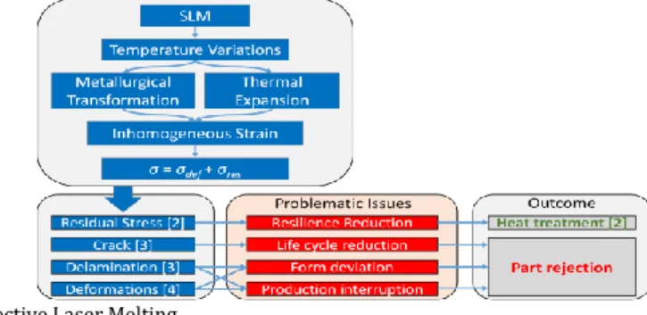
Contrary to conventional methods, the costs of Additive Manufacturing (AM) are not significantly influenced by increased part complexity [1]. Selective Laser Melting (SLM) is a common process of AM and is therefore studied in this work. It involves a step by step deposition of metal powder layers by a recoater (soft or hard). At each step, a laser beam scans the required area of the deposited powder to melt it locally. Next this area cools and solidifies to become a layer of the manufactured part. Thus, the SLM process involves high variations of temperature. As shown in Fig. 1, it induces thermal expansion of the material and phase transformations. Both phenomena generate inhomogeneous strains during solidification of molten metal that cause an overall residual stress field.
These stresses create four problems of which only the first one may be limited after production. The first impediment is the reduction of the strength of the manufactured part due to residual stresses. As discussed by Mercelis and Kruth [2], it may be lowered by rescanning of the layers during manufacturing or heat treatment of the part. The second problem is the reduction of the lifespan of the piece which may be linked to micro-cracks and micro-delaminations [3]. Third impediment pertains to the deviations from the nominal form of the produced part [4]. Last problem is production interruption due to a collision between the recoater and the manufactured part that may be caused by part deformations, protruding from the actual powder layer.
Several works were dedicated to the prediction of the distortions of SLM parts, but most studies [5–7] are limited to a simple specimen geometry: i.e. a single rectangular layer. They are based on thermomechanical Finite Element (FE) simulations of SLM process and mainly differ by the exploitation of the results. Matsumoto et al. [5] presented the deformation indirectly, as a ratio of deflection to laser diameter. Parry et al. [6] performed a calculation of stress and strain fields. However none of these works offer an experimental validation of stress and strain fields. A similar computation was too accomplished by Li et al. [7] who also provided a validation based on the normalized deformation in both scanning directions. SLM process does not consist of a single layer coating but involves the superposition of multiple layers. Thermomechanical FE models were therefore already developed in several studies to predict the strains and stresses induced in a rectangular block. In such work, Fateri et al. [8] compared the maximum form deviation predicted by the model to the value measured on a real part. A simulation of the complete residual stress field was also realised by other authors, such as Bartel et al. [9], but the results were not validated experimentally. Industrial parts rarely consist of a single rectangular block. There is a limited number of works concerning parts with a complex geometry. A multiscale thermomechanical FE model was
however developed by Li et al. [10] to simulate the 3D printing of a L-shaped bar and a bridge specimen. The experimental and simulated values of the curling angle of the bridge specimen were thus compared, but whole shape deviations of the part were not considered. Hodge et al. [11] proposed a thermomechanical model coupled with an analytical solution to laser irradiation on the powder material. The stress was derived from an elastoplastic constitutive law. The simulated deformation of a triangular specimen was then compared to data measured on a real sample. The authors concluded that the results are encouraging but present certain discrepancies with the experiments. All in all, there is a lack in the existing literature of a validated FE model that accurately predicts the complete form deviations of a part.
In first section of this paper, a thermomechanical FE model is proposed to predict the deformation of complex parts manufactured by SLM. As in the process itself, the simulation works in a layer-by-layer sequence. These layer-by-layers are connected between each other through activated contact elements. In second section, a simple macroscopic deformation experiment is defined to account for the complex metallurgical phenomena. The model does not need to use plastic hardening to reproduce the experimental results. Last section consists of an experimental validation based on an asymmetric tubular sample whose geometry looks like the one of a real industrial part. The shape of the SLM part is measured and compared to the geometry predicted by the proposed FE model.
2. Definition of thermomechanical model of SLM process
2.1. Theoretical basis
As shown in Fig.1, in SLM, the deformations of parts can be connected to thermal loads and metallurgical transformations.
Fig. 1. Challenges in the Process of Selective Laser Melting.
The prediction of thermal deformations is commonly carried out using a thermal expansion coefficient. On the other hand, metallurgical transformations of steels are complex to model and requires an in-depth knowledge of the phase changes. The proposed approach is therefore to combine both deformations in a single macroscopic term. To simplify the illustration, these phenomena are presented in a single dimension in Fig. 2, even though the model is defined in three dimensions. Thermal cooling usually generates a contraction. However, due to phase transformations the global deformation may result in contraction or expansion. This depends on the alloy composition and the cooling path.
At each manufacturing step, the total layer length mismatch Ltotal corresponds to the difference between the length of the cold sublayer Lcand the size of the hot layer Lh(Eq. 1). Ltotalcan also be divided into a thermal deformation, Lth, and the deviation due to the metallurgical transformations,
me
L
. The thermal deformation is deduced from Eq. 2, based on the hot layer temperatureTh, the cold layer temperature Tc and the thermal expansion coefficient . The metallurgical effects are described by a temperature mismatch. A virtual temperature Tme is defined to this end (Eq. 3). Tme may be lower or higher than Tc to describe an expansion or contraction of the material. Ltotal(Eq. 4) is obtained by the combination of Eq. 1, 2 and 3. To account for both phenomena (thermal and metallurgical), we propose to merge them into a macroscopic thermal deformation. In the proposed FE model, this
deformation is driven by the macroscopic temperature variation, Tmacro. Also, the nominal value of the thermal expansion coefficient is kept (Eq. 4).
total c h th me L L L L L = − = + (1) ( ) th c h h L T T L = − (2) ( ) me c me h L T T L = − (3) ( ) ( ) ( ) 2 2 total c h me h total macro h macro c h me L T T T L L T L T T T T = − + = = − + (4)
Therefore, Tmacro must be calibrated to fit the overall process parameters (see section 3). Even in three dimensions, the total strain total may be expressed, as the sum of a thermal strain th and a metallurgical deformation me(Eq. 5). Eventually, the difference in metallurgical structure of the calibration specimen and the SLM part may be a limitation of the proposed method. In fact, the metallurgical structure is driven by the cooling rate, which depends on the local geometry of the part.
me th
total th me total total macro
h h
L L
T
L L
= + = + = (5)
Fig. 2. Sources of deformations on the SLM final product.
2.2. Model Implementation
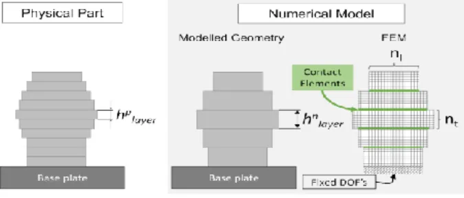
As previously mentioned, a thermomechanical FE model was employed in order to calculate the deformations of a complex geometry part produced using SLM. As in SLM process, the nominal CAD model’s volume is divided into layers of a thickness n
layer
h (see Fig. 3).
Fig. 3. Numerical model formulation.
To simulate the SLM process this thickness should correspond to the physical layer thickness, p layer
h
of the part. On the other side, to reduce the computing time, n layer
h may be chosen greater than p layer
h .
Hexahedral finite elements were used to mesh the layers. The number of elements in the direction of layer thickness, nt, is the same for all layers of the simulated part. In contrast, the number of elements
of edges on the interface of layers nl is adjustable. Thus, a refined mesh is applied on layers with
complex geometrical features. Layers with simpler geometry are described with a lower number of elements.
The areas of all layers that interface with one another, were meshed with thermally activated contact elements. It is important to note that contact elements are strictly surface elements and do not own any geometrical thickness. The contact elements are enabled when the temperature drops under a limit specified by the user. The laser/powder interaction and laser scan trajectory are not
simulated here. As presented in Fig. 4, each simulated layer geometry is stacked in its entirety at the beginning of each deposition step (timesteps t0, t2 and t4), in a hot state. Then the temperature is
decreased, and stress is accumulated within the model’s volume. To represent the contact with the SLM base plate, the first layer of the model is fixed at the bottom for the entire simulation. The temperature at the end of the cooling period is fixed to ambient (timesteps t1, t3 and t5).
Fig. 4. Thermomechanical behaviour of the model. 3. Thermomechanical model Calibration
3.1. Calibration process
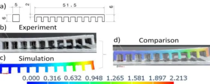
Each calibration result depends on the set of process parameters (e.g. material, scanning strategy, laser power). If one factor is changed a new calibration experiment must be carried out. The specimen used for the experimental calibration of the model is a flat rectangular beam of 2 mm thick, 6 mm width and 51.5 mm length (Fig. 5a). After manufacturing, the specimen is partially disjoined from the SLM base plate, using Electrical Discharge Machining (EDM). In order to avoid stress modification in the beam due to the EDM process, the sample is only maintained to the base plate by small rectangular supports. After manufacturing of the piece, the support structure is cut to a total length of 45mm. Only the last two supports are left intact. This cutting modifies the fixture of the beam; thus, due to stress present in the beam, the piece deforms. The beam is measured before and after its partial release, using a GOM ATOS III optical scanner (with an uncertainty of 18 µm). The maximum deflection value between these two datasets is the target of an iterative process for the fine tuning of
macro
T
. The iterative process modifies Tmacro until the difference between the simulated and experimental deformation is minimized. The obtained value of Tmacro accounts for all the process parameters (material, machine, lasing parameters, etc.). Naturally, it is necessary to use the same process parameters for the experimental calibration and the part to be simulated.
The experiment was conducted using 17-4PH steel. Young’s modulus E of this material is about 196 GPa, its Poisson’s ratio ν is 0.3 and its thermal expansion coefficient α is 10.8 µm/m °C. The experimental layer thickness was 30 µm. The laser power was fixed to 183 W. The scanning speed was set to 1,045 mm/s. The calibration model was meshed with 200,320 elements. The thickness of the layers used in the thermomechanical model was n
layer
h =350 µm.
3.2. Calibration Result
Fig. 5. (a) The geometry of the experimental calibration specimen, (b) the result of the experiment, (c) the nodal displacement of the FE model and (d)
the comparison of the deformation of the experimental specimen and the model’s result.
The distortion measured on the experimental part, after its partial release from the base plate, is illustrated in Fig. 5b. As shown in this picture, the deformation is significant and reaches several millimetres for a beam length of 51.5 mm. As stated previously, only two of the supports were left
intact. After the iterative procedure described in Section 3.1, the macroscopic temperature gap is calculated to simulate the same deviation (see Fig. 5c). This iterative process provided a value of temperature Tmacro=495 K. Fig. 5d. shows a comparison between calculated and measured sample shapes as obtained after EDM. It highlights the good agreement between the model and the experiment. The magnitude of the nodal displacement vector was 2.213 mm.
4. Experimental Validation
4.1 Validation Specimen Geometry
SLM process is more suitable for the manufacturing of thin complex structures. To be consistent with this type of parts, a validation specimen of complex geometry was designed. As shown in in Fig.
6, it consists of a tubular geometry with three prismatic holes. These holes, of 10 mm width, were
placed on one side only, rendering the piece asymmetrical. The total length of the piece was 61 mm. All the process parameters were the same as those used for the experimental calibration procedure (see Section 3.1).
Fig. 6. Geometry of the part used for the validation of the proposed methodology.
4.2 Finite Element Mesh Sensitivity Analysis
In order to evaluate the accuracy of the predicted sample distortions, a mesh sensitivity study was performed on the specimen defined in Section 4.1. Simulations were thus conducted with four different mesh sizes to analyse the influence of this factor on the maximum nodal displacement. The results of this study are shown in Fig. 7a. 203,526 elements were used in simulation Case 1 and 318,126 elements in Case 4 A difference of 2.4% has been found between the maximum displacement calculated in Case 3 and Case 4. This indicates that the model has converged to an asymptotic value.
Additionally, two views of the mesh used for Case 4 (most refined case) are presented in Fig. 7. As shown in Figs. 7b and c, it is important to notice that elements of neighbouring layers do not necessarily have to coincide in the interface. This is allowed, thanks to the use of contact elements. Hence, neighbouring layers may be described with mesh of widely different density.
Fig. 7. (a) Mesh sensitivity analysis, (b) the shape of the mesh used on the validation specimen and (c) detail of the elements located on the support
structure and the beam.
4.3. Qualitative Validation
Fig. 8a, shows a picture of the manufactured part in back and front view. The backside image
reveals significant distortions of the sample. In contrast, the front side of the real part was left relatively undeformed. Fig. 8b shows the contour plots of the predicted nodal displacements which are found to be similar to the distortions of the real part. The maximum predicted value of nodal displacements was 1.181 mm. It was located on the backside of the specimen. On the frontside of the
specimen there is only limited deformation. Moreover, the topmost part of the real part does not deform as predicted by the simulations.
Fig. 8. (a) Photographs of the experimental part: on the back side (top), on the front side (bottom) and (b) respective calculated nodal displacements.
4.4 Quantitative Validation
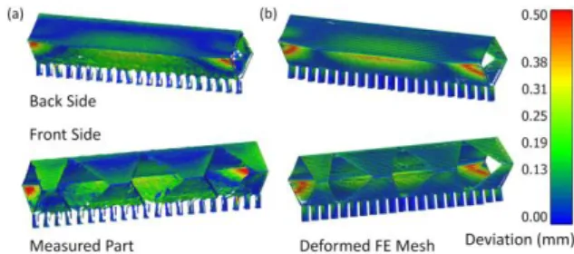
In order to evaluate the accuracy of the model, the manufactured part was measured using the optical scanner. A cloud of points was thus obtained and compared to the nominal CAD geometry. This data is presented in Fig.9a. On the other hand, the deformed mesh of the FE model was extracted and compared to the same nominal geometry (Fig.9b). The open source software CloudCompare v2.10 was used for that purpose.
Fig. 9. Distortions of the part in reference to the nominal geometry (a) of the real measured part and (b) the deformed FE mesh.
Fig.9 shows that the predicted distortion field well fits the experimental one and this on the entire
part. The highest deformation was predicted at the end points of the back-side edge. At this location both the real piece and the simulation show a distortion of approximately 0.5 mm. At both extreme zones of the front side, the value measured on the real part is about 0.19 mm, while the simulation predicted 0.13 mm.
Fig. 10. Comparison between the measured surface of the specimen and the deformed mesh of the FE model expressed as (a) a contour plot and (b) as
the distribution of samples versus the deviation per maximum calculated deformation.
Next, a comparison between the predicted and the measured distortions was made and depicted in a contour plot (Fig. 10a). The results suggest that, overall, the difference between the measurements and the prediction is limited to 10% of the maximum displacement value. Locally, the difference may reach higher values (e.g. at the end points of the back-side edge) which may be explained by local melting defects. In Fig. 10b the distribution of the differences between predicted and measured distortions, is presented. This histogram shows that the form defects were accurately predicted by the simulation.
5. Conclusions
The computational thermomechanical model proposed in this work made it possible to accurately predict the dimensional distortions induced by manufacturing of a complex 3D part with SLM process (less than 10% of maximum difference).
The proposed method is based on:
• A thermomechanical FE model which works in a layer-by-layer basis, like SLM process
• Thermally activated contact elements, used to model the interaction between successive layers • A simple experimental calibration process used to represent the complex thermomechanical
phenomena arising during the SLM process
In particular, the proposed model provides a good basis for performing calculations for parts with complex geometry. The capability of the proposed approach to simulate a variety of materials must however be validated in future works. A significant limit of the proposed method regarding industrial parts is also the high computing time (25 hours were needed in our study to perform the calculations on a PC laptop). Finally, this method seems to offer a promising tool to predict residual stresses induced by SLM process. This work represents a step toward a digital twin.
Acknowledgements
This work has received funding from the Excellence Initiative of Aix-Marseille University - A*Midex, a French “Investissements d’Avenir” program. The experimental equipment was funded by the European Community, French Ministry of Research and Education and Aix-Marseille Conurbation Community. Finally, the authors would like to acknowledge the contribution of Quentin-Alexis Lopez to the manufacturing of the specimens.
References
[1] Thompson, M. K., Moroni, G., Vaneker, T., Fadel, G., Campbell, R. I., et al., 2016, Design for Additive Manufacturing: Trends, opportunities, considerations, and constraints, CIRP annals, 65/2:737–760.
[2] Mercelis, P., Kruth, J.-P., 2006, Residual stresses in selective laser sintering and selective laser melting, Rapid prototyping journal, 12/5:254–265.
[3] Dadbakhsh, S., Hao, L., Sewell, N., 2012, Effect of selective laser melting layout on the quality of stainless steel parts, Rapid Prototyping Journal, 18/3:241–249.
[4] Aidibe, A., Tahan, A., Brailovski, V., 2016, Metrological Investigation of a Selective Laser Melting Additive Manufacturing System: A Case Study, IFAC-PapersOnLine, 49/31:25–29.
[5] Matsumoto, M., Shiomi, M., Osakada, K., Abe, F., 2002, Finite element analysis of single layer forming on metallic powder bed in rapid prototyping by selective laser processing, International Journal of Machine Tools and Manufacture, 42/1:61–67.
[6] Parry, L., Ashcroft, I. A., Wildman, R. D., 2016, Understanding the effect of laser scan strategy on residual stress in selective laser melting through thermo-mechanical simulation, Additive Manufacturing, 12:1–15.
[7] Li, C., Liu, J. F., Guo, Y. B., 2016, Prediction of Residual Stress and Part Distortion in Selective Laser Melting, Procedia CIRP, 45:171–174.
[8] Fateri, M., Hötter, J.-S., Gebhardt, A., 2012, Experimental and theoretical investigation of buckling deformation of fabricated objects by selective laser melting, Physics Procedia, 39:464–470.
[9] Bartel, T., Guschke, I., Menzel, A., 2018, Towards the simulation of Selective Laser Melting processes via phase transformation models, Computers and Mathematics with Applications, 78/7:2267–2281.
[10] Li, C., Guo, Y., Fang, X., Fang, F., 2018, A scalable predictive model and validation for residual stress and distortion in selective laser melting, CIRP Annals, 67/1:249–252. [11] Hodge, N. E., Ferencz, R. M., Vignes, R. M., 2016, Experimental comparison of residual stresses for a thermomechanical model for the simulation of selective laser melting,