HAL Id: hal-01966351
https://hal.inria.fr/hal-01966351
Submitted on 28 Dec 2018
HAL is a multi-disciplinary open access
archive for the deposit and dissemination of
sci-entific research documents, whether they are
pub-lished or not. The documents may come from
teaching and research institutions in France or
abroad, or from public or private research centers.
L’archive ouverte pluridisciplinaire HAL, est
destinée au dépôt et à la diffusion de documents
scientifiques de niveau recherche, publiés ou non,
émanant des établissements d’enseignement et de
recherche français ou étrangers, des laboratoires
publics ou privés.
Immersed in Complex Topography using Non-Rotative
Actuator Discs
Cyril Mokrani, Mireille Bossy, Marcos Di Iorio, Antoine Rousseau
To cite this version:
Cyril Mokrani, Mireille Bossy, Marcos Di Iorio, Antoine Rousseau. Numerical Modelling of
Hydroki-netic Turbines Immersed in Complex Topography using Non-Rotative Actuator Discs. Three Years
Promoting the Development of Marine Renewable Energy in Chile 2015 - 2018, MERIC-Marine Energy
and Innovation Center, 2019, 978-956-09327-0-9. �hal-01966351�
Topography using Non-Rotative Actuator Discs
ICyril Mokrania,∗, Mireille Bossyb, Marcos Di Iorioa, Antoine Rousseauc
aMarine Energy Research and Innovation Center, Avenida Apoquindo 2827, Santiago, Chile bInria Sophia Antipolis M´editerran´ee, Universit´e Cˆote d’Azur, France
cInria Sophia Antipolis M´editerran´ee, Montpellier, France
Abstract
Recent studies have pointed out the potential of several coastal or river areas to provide significant energy resources in the near future. However, technological processes for extracting energy using Marine Current Energy Converters (MCEC) are not generically “field-ready” and still require significant research to be set up. The present work comes within this framework: we develop the numerical model OceaPoS, useful to carry out a comprehensive description of turbulent flow patterns past MCEC and forward optimize the turbine arrays configurations and evaluate their environmental effects.
The OceaPos model consists in describing the fluid as an ensemble of Lagrangian particles ruled by a Stochastic process. OceaPos follows the same methodology than SDM–WindPoS model for wind farm simulations and adapts the Lagrangian stochastic downscaling method (SDM) ofBossy et al.(2016,2018) to the tidal and oceanic boundary layer. We also introduce a Lagrangian version of actuator discs to take account of one or several MCEC’s devices and their effects on the flow dynamics. Several benchmarks are presented, and numerical predictions are compared to experimental results.
Keywords: Tidal and oceanic turbulent flow; Stochastic numerical model; Hydrodynamics; Turbulent flows, Stochastic Lagrangian models; Marine current energy converters.
Contents
1 INTRODUCTION 2
2 NUMERICAL METHODS 4
2.1 Numerical approach . . . 4
2.2 Method for including bathymetry effects on the flow . . . 4
2.3 Model of hydrokinetic turbines . . . 5
3 GENERATION OF THE BOUNDARY LAYERS 6
3.1 Experiments. . . 6
3.2 Results. . . 7
IThis work was supported by Marine Energy Research and Innovation Center (MERIC) project L1.6 Advanced modelling
for marine energies. This paper is a part of the MERIC - 2018 Report.
∗Corresponding Author
Email addresses: cyril.mokrani@meric.cl (Cyril Mokrani), Mireille.Bossy@inria.fr (Mireille Bossy), marcos.diiorio@meric.cl (Marcos Di Iorio), antoine.rousseau@inria.fr (Antoine Rousseau)
4 INFLUENCE OF BATHYMETRY ON THE FLOWS 7
4.1 Experiments. . . 8
4.2 Results. . . 9
5 CASES INVOLVING NON-ROTATIVE TURBINE(S) 10
5.1 Experiments. . . 10
5.2 Results. . . 11
6 CONCLUSION 11
1. INTRODUCTION
Technologies for extracting energy from tidal currents using hydrokinetic devices have not yet achieved a sufficient degree of maturity to enable their widespread integration into power grid interconnected systems (Khan et al.,2008), (G¨uney and Kaygusuz,2010). Recent studies have identified potential in many coastal areas which could provide significant renewable energy resources in the near future, although their imple-mentation would require the overcoming of challenging technical, environmental and economical aspects, all of them site-specific.
Along the 6,400 km coast of Chile, in the South Pacific Ocean, the Chacao Channel has, according to initial estimates (Cruz et al., 2009), been identified as an important energy source that could potentially contribute to a total power capacity of between 600 and 800 MW. Motivated by the need to learn more about the physical and environmental processes of highly energetic areas similar to the Chacao Channel, we are developing a numerical model that aims to comprehensively describe flow past turbines for a wide range of scales, to optimise turbine arrays and evaluate their environmental effects.
To improve device installation and performance through numerical predictions, it is necessary to model turbulence flows. Indeed, the Chacao Channel presents current velocities of up to 10 m/s at high tide and a complex bathymetry with high depth variations, which naturally generates turbulent flows. In addition, this ambient turbulence may be significantly increased by turbine blade interaction with the incident flow, mainly due to high shear stress generated downstream from the turbine.
Among the existing numerical methods for modelling turbulent flows, one can separate the Eulerian Averaged Models (EAMs) and Lagrangian Stochastic Models (LSMs). Those two approaches are fundamen-tally distinct for various reasons: first, Eulerian methods compute solutions (velocity and pressure fields) on a fixed mesh grid (see Figure1-(a)) and thereby provide a snapshot of the flow at every instant. Conversely, Lagrangian methods follow water particles during the simulation and compute their velocity at each time step. Contrary to Eulerian models, the Lagrangian approach provides the trajectory (positions) of fluid particles (see Figure1-(b)).
In addition, EAMs provide pressure and velocity fields averaged over a characteristic duration or length (chosen a priori i.e., as input parameter ). This is equivalent to saying that only large-scale turbulent processes are solved. Small-scale effects are included in the EAM’s description, however they are “added” to the numerical solutions through an additional input variable (see Reynolds tensor or sub-grid tensor). Conversely, the LSM computes instantaneous fields of each water particle, and provides solutions which include both large and small-scale turbulent effects. An important point is that it is possible to deduce averaged fields from LSM solutions but not vice-versa.
Among the EAMs, the Reynolds-averaged Navier-Stokes (RANS) (Zahle and Sørensen,2011) and Large-Eddy Simulation (LES) methods (Sezer-Uzol and Long,2006) have been widely developed to model turbulent flows induced by tidal turbines. LES have been used to model blade motions, predict forces and torque in-duced on the stator (Sezer-Uzol and Long, 2006; Kang et al., 2012), and improve the prediction of the
Figure 1: Two different approaches used to model turbulent flows – (a) Eulerian approach, (b) : Lagrangian approach.
power generated by the turbine (Kang et al.,2012). RANS models have also provided excellent predictions, especially regarding the local flow/structure interactions occurring during the extraction process.
However, these methods have proved to become very intensive and demanding in terms of computational resources. Accurate predictions of RANS require at least 6 million grid nodes, with a large number concen-trated in the wake region (Turnock et al., 2011). This requirement can be even more important for LES models, for which a total of 185 million grid nodes are required to resolve the flow field around one single turbine device (Kang et al.,2012). These computational needs clearly lead to prohibitive computation pro-cessing times, which becomes unfeasible if multiple interacting turbines are considered in the simulation. So far, the need to reduce the demand on computer resources for EAMs has motivated a number of researchers to propose innovative methods such as coupling approaches or hybrid methods with the objective of saving computational resources associated to EAM.
Contrary to EAMs, LSMs are more recent and fewer studies have been published so far. LSMs have been originally developed byPope(2000), based on stochastic differential equations whose solutions are the instantaneous positions and velocities of fluid particles. The main usage of LSM models in engineering is to provide information for the instantaneous velocity of the flow seen by dispersed physical particles. Such approaches have been extensively used for turbulent flows in combustion engineering, in association with an EAM for the computation of the mean flow information (Minier,2016). Recently a stand alone version of LSM has been developed as a simulation solution for turbulent flows and mainly applied to atmospheric flows: Polagye et al.(2011) used a LSM for meteorological frameworks and predicted turbulent flows fields in a realistic case of wind refinement. Originally, standalone LSM for wind computation is a downscaling method, that provides a local model limited to a given region, forced by meteorological large scale infor-mation. In order to reconstruct the mean flow field from the fluid-particle motion, a Particle-in-cell (PIC) technique is retained (see further details in Bossy et al. (2016)) that introduces a fixed mesh according to some characteristic flow length. Zahle and Sørensen (2011); Bossy et al. (2018) computed the wind circulation around mills and obtained very promising estimations of the wind variability in the wake of a wind turbine. However, even now, no studies based on tidal or ocean flow are available and the question of LSM ability to describe turbulent flows generated by tidal turbines remains unresolved. More important is the assessment of their performance. Given the high computational times associated to EAMs, reducing computational times should be very welcome.
The present study aims to evaluate the performance of the LSM “Stochastic Downscaling Method – Ocean Power Simulation (SDM–OceaPoS)” with the purpose of developing an inexpensive computation tool capable of simulating interaction between high Reynolds flows with both multiple turbine devices and com-plex bathymetry.
Section 2 provides details of the numerical methods employed in this study. Section 3 presents one verification case based on the boundary layer generation. Sections4 and5 present two benchmarks, based respectively on turbulent flows generated by a bathymetry (from Almeida et al. (1993); Loureiro et al.
(2007)) and instantaneous wake dynamics generated by an non rotative turbine (from Myers and Bahaj
(2010, 2012)). Since Section II is a preliminary study, conversely Sections IV and V intend to establish a framework for future optimisation of turbine arrays on specific sites.
2. NUMERICAL METHODS 2.1. Numerical approach
The development of the SDM–OceaPoS model is based on an existing code that models air flows named SDM–Windpos. The “air” version has been validated on atmospheric flows (Bossy et al.,2016), although its translation to the water version is still under development.
In the current version, the water is described as an incompressible flow by a Lagrangian approach. The Lagragian description of the flow uses stochastic diffusion processes given as the solution of a stochastic differential system (we refer the interested reader toBernardin et al.(2010) for a mathematical description of the method, and to Pope (2000, Ch. 12) to a physical introduction to this methodology). The time evolution of particle velocities is described and computed from three acceleration terms, including (i) the pressure gradients contributions, (ii) the advective and convective effects of the fluid displacement, and (iii) a diffusive term governed by a Brownian motion. These three terms allow to take both small and large scale turbulent processes into account in the simulations.
One of the main advantages of the SDM–OceaPoS approach is that in addition to providing the instanta-neous fields particles, it also provides averaged fields, similar to a classical EAM. This Eulerian description of the flow is possible thanks to a fixed regular mesh grid superposed to the numerical domain. During the computation, spatial averages of Lagrangian velocities of particles located in the same cell are assessed, together with the variance and covariances. These Eulerian fields are computed at each time step after particle advections. In practice the number of particle in each cell keeps constant in order to guarantee the incompressibility constraint. This step is performed using particle optimal transport algorithm (seeChauvin et al.(2010) for a description of proposed algorithms and Bossy et al. (2013) for a mathematical descrip-tion of incompressible Lagrangian stochastic model). Using this approach, the user has to set two input parameters which are (i) the mesh size used to assess the Eulerian fields, and (ii) the number of particles per cell.
2.2. Method for including bathymetry effects on the flow
SDM–OceaPos uses a wall treatment method to reproduce the momentum exchange present in the inter-action between fluid particles and arbitrary bathymetries. The method implemented consists of reflecting any particle that enters into a region close to the ground (namely the “mirror region”). Outside this region, particles are in the fluid domain and describe the fluid dynamics. Inside the mirror region, the flow not is solved, however its effects are included in the fluid domain simulations. To make it possible, a 3-dimensional topology file is first generated prior to the computation with the main ground characteristics (that is to say, the ground position, the ground local inclinations, and the frictions coefficients). During the computations, SDM–OceaPos assesses each reflected velocity of particle that cross the mirror region from the input ground data. This step is performed by assuming that the covariances before and after the reflection keep equal.
This method is applied in three steps : (i) SDM–OceaPos first detects particles that enter the sub-viscous layer at a given iterative step. During this step, the position the particle would reach without terrain (the virtual position) is computed. (ii) The position of the reflected particle is calculated according to the local ground inclination, and hit virtual position. The particle is then re-introduced into the fluid domain. (iii) The reflected velocity vector is computed according to the friction and the covariances assessed before the
reflection.
This original method is applied in Section III on a case involving a 2D hill introduced in a turbulent flow.
2.3. Model of hydrokinetic turbines
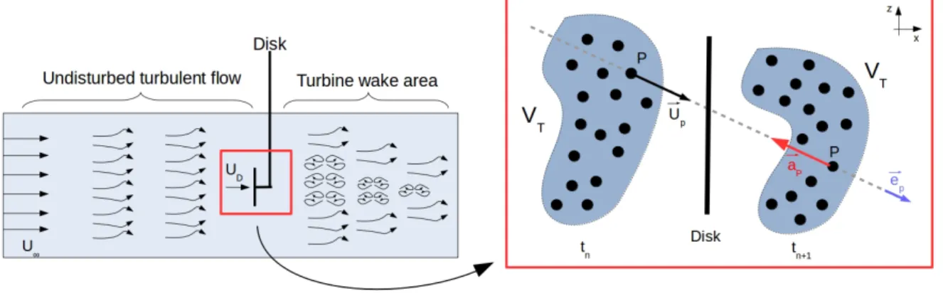
The implemented model of a non-rotative turbine is based on the theory of porous discs (Myers and Bahaj,2010,2012). Such discs, introduced into a turbulent flow, may disturb the flow field by generating a turbulent wake as illustrated in Figure2-(left).
Turbine models were initially implemented in the air version of SDM (Bossy et al., 2016). They con-sisted in applying a correcting velocity to particles located at the disc location. This correcting velocity was assessed from an theoretical expression of the force generated by the disc on the fluid. However several problems related to this approach have been pointed out: first, this corrected velocity was added after the advection step, and therefore the turbulence generated upstream from the disc was generated indirectly by the velocity deficit, but not by the disc himself. This may lead to a misrepresentation of the wake recov-ery and impacts in realistic scenarios. Other limitations were that the corrected velocity was applied in a fixed control volume – typically the disc volume – and therefore any particle crossing the disc without staying in this control volume was not corrected. This not only provided a non realistic behaviour of the fluid particle, but also resulted in a flow description of flow very sensitive to the space step and the time step. A new approach has been developed to solve these problems. It involves adding an acceleration source term to the momentum equation. In this manner, the turbulent effect induced by the turbine itself can be included in the simulation. Additionally, this source term is applied to a new control volume, defined as the volume of all particles that cross the disc between two iterative steps. With this variable control volume any particle that crosses the disc “feels” its effect.
From a mathematical point of view, the source term acceleration is assessed from the ratio between the total force applied on the control volume and its corresponding total mass, as illustrated in Figure2-(right).
Figure 2: Illustration of the wake generated by the porous disc (left), and (right) the approach of the implemented model: particle accelerations are estimated from the total force applied on the volume VT. The direction of the particle’s force is aligned with the disc-crossing particle velocity.
• The expression of the total force is given in Simisiroglou et al. (2016). For the present study, this force is assumed to be exerted in the direction of the disc-crossing particle velocity, as indicated in Figure2. Usually the force is given according to the porosity coefficient, the area of the disc and the fluid velocity vector in the disc’s vicinity. However, for the present model we used the induction factor (denoted a, seeBossy et al. (2016)) instead of the porosity coefficient because this coefficient allows for the linking of the instantaneous particle velocities at the disc location (see UD in Figure2-(left))
to the particle velocity away from the disc (see U∞ in Figure2-(left)).
• The total mass of the control volume is estimated by the product between the total number of par-ticles that cross the disc and the mass of one single particle. The latter is calculated by assuming that the volume of each grid cell equals the sum of the volumes of all particles in this cell. From this assumption, the particle mass can be easily deduced.
Finally, the corrected acceleration term is re-assessed at each time step for each particle that crosses the disc. This approach allows for obtaining a flow description independent from the numerical input param-eters: when changing the mesh grid size (respectively the time step), the control volume changes and the subsequent acceleration keeps the same order of magnitude so that the effect of the disc on the flow remains similar.
In the following, one verification test (Section3) and two benchmarks (Sections4 and5) are presented. All numerical computations have been performed with the multi-threaded open Multi-processing (openMP) version of SDM–OceaPoS, and using 23 cores, having a frequency of between 2 and 2.4 GHz. The hydroki-netic turbine model is applied in Section5 for cases involving turbine diameter D of about one third of the depth h (D ' h/3).
The next section is dedicated to benchmarks carried out on cases of flows without turbines. Emphasis is placed on the generation of boundary layers and the effects of a given bathymetry on a turbulent flow.
3. GENERATION OF THE BOUNDARY LAYERS
A first study has involved considering verification test cases in order to assess the ability of SDM to re-produce the basic physics of a turbulent flow without turbine. The objective is to re-create experiment in channel and assess the numerical accuracy of the computed velocity fields by comparing numerical and theoretical results.
3.1. Experiments
The following results are based on the experimental study from Nezu and Rodi (1986) (see Figure 3 -(left)). It involves 2D flow evolving in a 20 m long, 60 cm wide and 65 cm deep open channel with smooth ground. During experimental tests, the water is stably recirculated with maximum discharge reaching 80 l/s, which generates a turbulent flow with a Reynolds number of about Re ' 104. The friction velocity is assessed
at 0.44 cm/s.
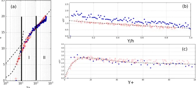
Results fromNezu and Rodi(1986) show the generation of mainly four boundary layers in a steady state (see Figure3-b) whose structures depend both on the ground roughness and interface motion. The ground roughness generates the viscous sub-layer in which the velocity profile follows a linear law. Above this first boundary layer, a transition region appears in which the velocity profile tends towards a classical “log” law. Above the log-law region, the free-surface motion disrupts the velocity profile resulting in a new boundary layer (seeNezu and Rodi(1986)). For the present study, one focuses only on the intermediate, and log-law regions and neglects the effect of the free-surface and the sub-viscous layer. The latter assumption is justified
Figure 3: Sketch of the experiment fromNezu and Rodi(1986) (left). Theoretical average velocity profiles in each sub-layer of a turbulent 2D flow (left) – y+= yU∗/ν, U+= U/U∗, with U∗= 0.44 cm/s.
by the fact that the sub-viscous layer has very small dimensions in relation to those of the turbine deployed in this study (D ' h/3).
3.2. Results
Numerical tests have been made using the parametrisation of the turbulent viscosity proposed in the study fromNezu and Rodi (1986) derived from laboratory measurements. Computations have been per-formed using 128, 000 cells in total, and 80 particles per cell in a numerical domain of ' 1 m3.
Figure4presents the mean velocity profiles and variances of the vertical and horizontal velocities. The-oretical solutions are also represented in the same figure in order to assess the numerical accuracy to model the boundary layers. As observed, results from SDM–OceaPos provide excellent trends of velocities in the intermediate and outer log-law regions of the flow. Mean velocity predictions are slightly under-predicted in the interface vicinity, since the effect of interface on the flow is neglected. Also, the sub-viscous layer is poorly modelled due to the assumption previously mentioned. Maximal relative error according to theoret-ical results reached less than 10%.
Variances of horizontal and vertical velocity are compared to the mean velocities fluctuations in Figure4
(b) and (c). Both global trends and order of magnitudes are in good agreement with theoretical values. Maximal error reach about 13% compared to theoretical results.
Regarding the numerical performances, all computations have been performed over 200 iterations using a constant time step of 0.2 s. The corresponding time calculation for one iteration is about 0.05 s, which means that one second in the physical experiment could be modelled in about 0.25 s.
Finally, these predictions, together with the corresponding performances observed lead to the conclusion that the main structure of a high Reynolds number flow can be accurately reproduced at very reasonable computation times.
4. INFLUENCE OF BATHYMETRY ON THE FLOWS
The second tests are focused on the influence of the bathymetry on the flow, modelled by using the numerical method presented in sub-section2.2. It involves reproducing the experiments performed in the laboratory and comparing them to the numerical predictions. The objective is to assess the ability of SDM–OceaPos to describe the turbulent flow dynamics involved in controlled configurations.
Figure 4: Comparisons between numerical predictions (•), theoretical predictions (–) and measured (++) mean velocities (a), averaged horizontal (b) and vertical (c) fluctuations velocities in intermediate I and II outer sub-layers flow - Y+ = yU∗/ν, U+= U/U∗, with U∗= 0.44 cm/s, and h = 10 cm.
4.1. Experiments
All numerical results presented hereafter have been compared to experimental measurements performed byAlmeida et al.(1993);Loureiro et al. (2007). These studies consider a 2D hill placed in a water tunnel to measure its effects on turbulent flow (see Figure5-a).
Figure 5: (a) Visualisation of the considered flow with hill (Almeida et al.,1993)- (b) Zoom of the downhill zone and illustration of the recirculation zone generated by the presence of the hill (Loureiro et al.,2007).
The water tunnel is made of perspex and is 0.170 m deep, 0.2 m wide, and 7 m long. During the experi-ments, the water flow passes through straighteners located upstream of the duct inlet in order to ensure hit uniformity. Experiments correspond to Reynolds number flows of about 6.104. The model hills are made of plastic moulded with a wooden former. Their shape corresponds to the inverse of a fourth-order polynomial function, with a maximal height and length in the streamwise direction of 28 mm and 108 mm respectively. During the experiment, the curvature of the flow affects the velocity field, which results in the estab-lishment of a zone of high-intensity velocity fluctuations along the shear layer downstream of the top of each hill. The hydrodynamical effects of the hill on local turbulence can be observed in Figure5, especially the emergent structures upstream and the recirculation zone downstream of the hill. Two specific points,
named detachment and reattachment points, are defined as the positions where the shear stress changes sign. These points determine the main flow structure generated by the hill. According to Loureiro et al.
(2007), the detachment point extends up to x/h = 4.8, as can be observed in Figure5(b).
Figure 6: Stream lines estimated from experimental measurements (Almeida et al., 1993; Loureiro et al.,2007) (a) and calculated by SDM–OceaPoS (b) - The maximum input speed is U0= 2.147 m/s, and the height of the hill is h = 28 mm.
Figure 7: Vertical profiles of horizontal velocities at different x positions of the domain (x = 0 m –corresponds to the position of the center of the hill) - (-): Numerical predictions, (•): Measurements fromAlmeida et al.(1993) (h = 28 mm).
4.2. Results
The following results correspond to computations performed using 96, 000 cells in total and 50 particles per cell. To reduce convergence times, a first computation was done without a hill and stopped when all the mean velocity, first and second order moments fields reached stabilised trends. These fields were imposed both as a boundary at the left side of the domain, and initial state in the whole domain.
Simulations including the hills have been performed using smaller time steps and more iterations to obtain converged results. In total, we ran 2, 000 iterations which lasted about ' 5 hours. This corresponds to a CPU rate of 9 iterations per second.
Figure 6 shows the stream lines obtained after 1, 000 iteration steps. It can be observed that the re-circulation zone is well described by the code and that its dimensions are very close to those observed experimentally. The detachment point location has been assessed at 4.28 h against 4.8 h fromLoureiro et al.
(2007). The generation and stabilisation of this recirculation zone proved to be sensitive to the time step parameter, especially when low values of this parameter were set. Using the value dt = 0.0005 s provided a stable computation and resulted in positive alignment with laboratory data.
Figure 7 presents the vertical profiles of the mean horizontal velocity predicted at different locations upstream and downstream of the hill. As observed, numerical predictions are very close to measurements for all the considered distances to the hill. Maximal error on the mean velocity is about 10% and is reached at the hill top.
The interested reader can find more information about this benchmark case inDi Iorio et al..
5. CASES INVOLVING NON-ROTATIVE TURBINE(S)
The following validation tests are based on experiments from Myers and Bahaj (2010, 2012) involving porous discs introduced in a turbulent 2D flow. In order to estimate the ability of SDM–OceaPos to describe both the velocity deficit and the turbulent intensity generated by one or various porous disc(s), we reproduced similar experiments using the method presented in Sub-section2.2.
5.1. Experiments
Myers and Bahaj (2010, 2012) carried out flow measurements in the wake of the discs to determine the flow recovery as a function of the thrust produced by the devices and analyse flow interaction in tur-bine arrays. The experiments were performed in a 21 m long by 1.35 m wide flume, with a water depth of
H = 0.3 m. The mean velocity of the flow equals 0.25 m/s, which yields a Reynolds number of Re = 75, 000
and a Froude number of Fr = 0.14 based on the flow depth H. Measurements were obtained by varying the number of discs, the disc immersion depth and the disc porosity. Figure8 shows the experimental set-up with one and three discs in the laboratory channel.
Figure 8: Experimental set-up of the research carried out by Myers and Bahaj(2010) – (a) Single disc configuration, (b) Three-discs configuration.
Diameter of the actuator discs (denoted AD in the following) remained constant, equal to D = 0.1 m for all tests that were performed. Porous discs were located in a section of the flume which had already reached a fully-developed turbulent channel flow. They were mounted on a rig with a pivot to amplify the forces and measure the total thrust with good accuracy. To vary the disc thrust, different porosities from 0.36 to 0.91 were tested using the same upstream flow conditions. The data provided also includes tests performed with different disc immersion depths. In any case, the measurement area extends from 3D to 20D downstream where instantaneous velocities were measured using a vertical resolution of 0.1H.
5.2. Results
The following results correspond to computations performed on a 275, 000 points grid and 100 particles per cell. For all cases, simulations were performed over 500 iterations with a time step of 0.1 s, which corre-sponds to a CPU rate of about one iteration per 10 s. The following figures correspond to results obtained at the last iteration of the computation.
Validation tests have been conducted by comparison analysis based on turbulence intensity and veloc-ity deficits. The velocveloc-ity deficit quantifies the velocveloc-ity reduction induced by the porous disc. The results presented are also compared to numerical predictions fromJohnson et al.(2014). The latter used a RANS numerical code with a k − ω turbulent model and a source term in the momentum equation to include the presence of the porous disc.
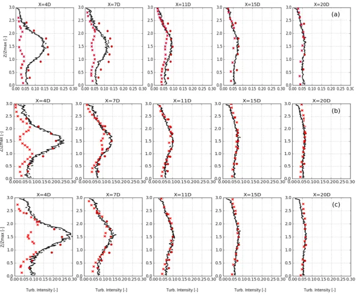
Figure 9 presents the vertical profiles of turbulent intensity computed and measured at different posi-tions upstream from the turbine. For this case, the porous disc immersion depth was half the total domain height. In general, numerical tests performed by SDM–OceaPoS provide very good predictions for all avail-able porosity values. The turbulent intensity is slightly under-estimated for low values of porosity coefficient. Conversely, they are overestimated for high values of CT, especially in regions close to the disc position.
Relative errors decrease away from the disc, reaching about 10% for CT = 0.62 and 8% for CT = 0.99.
Numerical predictions fromJohnson et al. (2014) provide a maximum relative error of 40% for turbulence intensity and 30% for speed deficit. In addition, they do not correctly reproduce turbulence intensity in the disc vicinity. Results obtained with SDM–OceaPoS are significantly better at this location.
Other results obtained on velocity deficit (not presented here) revealed corresponding maximum relative errors of the order of 7% for any porosity coefficient.
Figure 10 shows predictions of speed deficit where CT = 0.86 and the disc is immersed at mid-depth.
Comparisons with experimental data reveal that SDM–OceaPoS provides a good prediction of the spatial distribution of the speed deficit. The wake shape and dimensions are close to the experimental data. Low errors are observed, especially far from the disc or in the disc vicinity, where the deficit speed is slightly overestimated. Overall, the numerical results are fairly satisfactory.
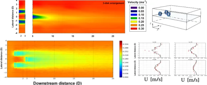
Similar conclusion can be drawn for cases involving various discs. Figure 11 presents results obtained for one case involving three discs disposed in a two-row array. The first row is two discs at 1.5D lateral separation and the second one is the third disc disposed downstream at a distance of 3D. As observed in Figure 11, for a downstream distance higher than 7D, numerical prediction of the velocity is in good agreement with experimental measurements. However, for a shorter distance, the numerical prediction is significantly over-estimated. For this case, further studies are needed to understand and improve results.
6. CONCLUSION
The present research aims to reproduce basic turbulent flows generated in rivers and seas both upstream and downstream of an AD device, by using a Lagrangian stochastic model. From the results obtained from one verification test and two benchmarks, it can be concluded that the SDM–OceaPoS model is able to accurately represent the flow structure generated at high Reynolds numbers, the effects of bathymetry on the mean velocity field in 3D cases and the effects of AD on the local turbulence generated past the turbine device. More specifically:
• The flow structure generated in a domain volume of about ∼ 1 m3 at a Reynolds flow of Re ' 104
could be described with a CPU rate of about one iteration per 0.05 seconds, with all computed mean horizontal and vertical velocities and variances properly predicted in intermediate and external bound-ary layers. These results were obtained by implementing the parametrisation of turbulence viscosity
Figure 9: Vertical profiles of turbulence intensity at different downstream positions of the turbine – (-): Numerical predictions from SDM–OceaPoS, (•): Measurements, (XX) : Numerical prediction fromJohnson et al.(2014) – (a) : CT = 0.62, (b) :
CT= 0.91, (c) : CT= 0.99 - Position x = 0 corresponds to the position of the disc center.
of Nezu and Rodi (1986), which does not include the presence of the interface, even if this does not seem essential for current industrial applications.
• A new method based on the reflection of particles has been validated using the experimental cases of Almeida et al. (1993); Loureiro et al. (2007), involving a 2D hill immersed in a turbulent flow. Present benchmarks showed that this method provides accurate velocity profiles both upstream and downstream from the AD device, with a maximum error of horizontal velocity reaching less than 10% at the top of the hill. The numerical simulations accurately describe the generation and stabilisation of the recirculating area, which shows that the present numerical model is able to predict the main turbulent pattern associated with this benchmark case. Together with previous results, this highlights the fact that SDM–OceaPoS can be used to predict the behaviour of most of the turbulent main flows observed in rivers and seas, without a turbine device.
Figure 10: Comparison of speed deficits of a porous disc of Ct = 0.86 predicted by SDM–OceaPoS (up) and measured in channel (Myers and Bahaj,2010) - Downstream distance is defined as (X − XD)/D where XDis the center disc position and
D the diameter of the porous disc.
Figure 11: Comparison of deficits in the case of three porous discs spaced by 1.5D - (top left): measured in channel (Myers and Bahaj,2012), (bottom left): Numerical predictions from SDM—OceaPoS, and (bottom right) : vertical profiles of velocity, (•) : Experimental, (–) : SDM–OceaPoS.
• A new turbine model has been implemented based on the porous disc theory. This model can reproduce with quantitative concordance all the features measured for channel flows with actuator discs used in the recent experiments of Myers and Bahaj (2010, 2012). The numerical solutions and comparisons with experimental data confirm the reliability of the PDF model in simulating turbulent flows gener-ated by AD devices. This model can resolve the mean flow velocity deficit and also the turbulence
statistics of the wake at high Reynolds numbers for various discs, while employing relatively low grid node numbers. The 3D dynamics of the flow field characterised by the asymmetric formation of arch vortices that emerge from the disc edges and interact downstream are properly reproduced only by adding an additional acceleration term in the Lagrangian equation of particle motion. This is very promising since these mechanisms are essential for predicting the interaction between the AD device and the environment. Another important concluding remark is that this approach, first developed for application in the atmospheric frame, can be easily adapted to ocean flows, especially by changing the parametrisation of the turbulent model. Moreover,predictions obtained by SDM–OceaPoS can be used to reconstruct water particle trajectories, which can yield an accurate description of physical processes inherent to turbulent flows generated from both an arbitrary bathymetry and also by a single or several AD devices (seeDi Iorio et al.).
Future work will focus on implementing an improved turbine model which includes the presence of ro-tating blades on a free-surface. In future, we expect this model to become a powerful tool for designing array turbines in the Chacao Channel and other similar sites, as it is ideally suited to better understanding the complex flows in natural marine environments, estimating available power and evaluating the impact of new technologies in local ecosystems.
References
Almeida, G., Durao, D., Heitor, M., 1993. Wake flows behind two-dimensional model hills. Experimental Thermal and Fluid Science 7, 87–101.
Bernardin, F., Bossy, M., Chauvin, C., Jabir, J., Rousseau, A., 2010.Stochastic Lagrangian Method for Downscaling Problems in Computational Fluid Dynamics. ESAIM: M2AN 44, 885–920.
Bossy, M., Dupr´e, A., Drobinski, P., Violeau, L., Briard, C., 2018. Stochastic Lagrangian approach for wind farm simulation, in: Forecasting and Risk Management of Renewable Energy. Springer Proceedings in Mathematics & Statistics, In press. Bossy, M., Espina, J., Morice, J., Paris, C., Rousseau, A., 2016.Modeling the wind circulation around mills with a Lagrangian
stochastic approach. SMAI-Journal of Computational Mathematics 2, 177–214.
Bossy, M., Fontbona, J., Jabin, P.E., Jabir, J.F., 2013.Local Existence of Analytical Solutions to an Incompressible Lagrangian Stochastic Model in a Periodic Domain. Communications in Partial Differential Equations 38, 1141–1182.
Chauvin, C., Bossy, M., Bernardin, F., Rousseau, A., 2010.Stochastic Downscaling Method: Application to Wind Refinement, in: Progress in industrial mathematics at ECMI 2008, Springer, Berlin. pp. 765–770.
Cruz, J., Thomson, M., Stavroulia, E., Rawlinson-Smith, R., 2009..Garrad Hassan .
Di Iorio, M., Bossy, M., Mokrani, C., Rousseau, A., . Particle tracking methodology for Lagrangian numerical simulations. Wave and Tidal - 3rd International Workshop, Nov 2018, Valdivia .
G¨uney, M., Kaygusuz, K., 2010. Hydrokinetic energy conversion systems: A technology status review. Renewable and Sustainable Energy Reviews 14, 2996–3004.
Johnson, B., Francis, J., Howe, J., Whitty, J., 2014. Computational actuator disc models for wind and tidal applications. Journal of Renewable Energy 2014.
Kang, S., Borazjani, I., Colby, J.A., Sotiropoulos, F., 2012. Numerical simulation of 3d flow past a real-life marine hydrokinetic turbine. Advances in water resources 39, 33–43.
Khan, J., Bhuyan, G., Moshref, A., Morison, K., Pease, J., Gurney, J., 2008. Ocean wave and tidal current conversion technologies and their interaction with electrical networks, in: Power and Energy Society General Meeting-Conversion and Delivery of Electrical Energy in the 21st Century, IEEE. pp. 1–8.
Loureiro, J., Soares, D., Rodrigues, J.F., Pinho, F., Freire, A.S., 2007. Water tank and numerical model studies of flow over steep smooth two-dimensional hills. Boundary-layer meteorology 122, 343.
Minier, J.P., 2016. Statistical descriptions of polydisperse turbulent two-phase flows. Physics Reports 665, 1–122.
Myers, L., Bahaj, A., 2010. Experimental analysis of the flow field around horizontal axis tidal turbines by use of scale mesh disk rotor simulators. Ocean engineering 37, 218–227.
Myers, L., Bahaj, A., 2012. An experimental investigation simulating flow effects in first generation marine current energy converter arrays. Renewable Energy 37, 28–36.
Nezu, I., Rodi, W., 1986. Open-channel flow measurements with a laser doppler anemometer. Journal of Hydraulic Engineering 112, 335–355.
Polagye, B., Van Cleve, B., Copping, A., Kirkendall, K., 2011. Environmental effects of tidal energy development. US Department of Commerce, NOAA Technical Memo, NMFS F/SPO , 186.
Pope, S.B., 2000. Turbulent flows. Cambridge University Press, Cambridge.
Sezer-Uzol, N., Long, L., 2006. 3-d time-accurate cfd simulations of wind turbine rotor flow fields, in: 44th AIAA Aerospace Sciences Meeting and Exhibit, p. 394.
Simisiroglou, N., Karatsioris, M., Nilsson, K., Breton, S.P., Ivanell, S., 2016. The actuator disc concept in phoenics. Energy Procedia 94, 269–277.
Turnock, S.R., Phillips, A.B., Banks, J., Nicholls-Lee, R., 2011. Modelling tidal current turbine wakes using a coupled rans-bemt approach as a tool for analysing power capture of arrays of turbines. Ocean Engineering 38, 1300–1307.
Zahle, F., Sørensen, N.N., 2011. Characterization of the unsteady flow in the nacelle region of a modern wind turbine. Wind Energy 14, 271–283.