Manual on the Basic Analysis of Agricultural Prices for Decision-making is published under license Creative Commons
Attribution-ShareAlike 3.0 IGO (CC-BY-SA 3.0 IGO) (http://creativecommons.org/licenses/by-sa/3.0/igo/)
Based on a work at www.iica.int
IICA encourages the fair use of this document. Proper citation is requested.
This publication is also available in electronic (PDF) format from the Institute’s Web site:
http://www.iica.int and http://www.mioa.org
Editorial coordination: Edgar Cruz Palencia.
Layout: Marilin Agüero Vargas.
Cover design: Marilin Agüero Vargas.
Print: IICA’ Print
San José, Costa Rica 2017
For the last fifteen years, national institutions involved in the management and operation of agricultural market information systems (MIS) have played a role, with varying impact, in the agricultural development of Latin America and the Caribbean (LAC). Their main tasks, which are to collect data and process and disseminate information, have served primarily as a catalyst for increasing agricultural productivity, but have also promoted the economic development of the countries through their respective productive sectors.
That same period saw the establishment of the Market Information Organization of the Americas (MIOA), a network conceived and supported from the outset by the Agricultural Marketing Service (AMS) of the U.S. Department of Agriculture (USDA). One of the main objectives of the AMS is to facilitate the efficient marketing of agricultural products in national and international markets, and it was this that prompted the network’s creation.
The MIOA has also become an important network for cooperation on training, comprised as it is of government and government-linked institutions whose chief responsibilities or objectives are the compilation, processing and dissemination of data related to agricultural markets and products. The institutions that are currently members of the MIOA network represent 33 LAC countries.
As part of its constant efforts aimed at innovation and the continuous improvement of processes, the Market Information Organization of the Americas (MIOA) is pleased to announce the publication of the “Manual on the Basic Analysis of Agricultural Prices for Decision-making” and make it available to its member countries. Its aim in doing so is to update and enhance the knowledge and technical expertise of officials responsible for operating trade information systems, to enable them to more effectively influence decisions taken by different market players and thereby make agricultural business activities more transparent. The manual is also designed to permit university students from different disciplines to study the basic concepts and gain a better understanding of the tools available for the analysis of agricultural prices, learn more about how markets function, and be better equipped to interpret the transmission of prices between products and markets.
Throughout this manual, the MIOA presents and analyzes different instruments and techniques of analysis that make it possible to better appreciate and understand the structure, behavior and operation of markets, particularly agricultural ones. It also considers the factors that determine the supply and demand for goods, the formation of prices, especially prices linked to agricultural products, and the types of market structure that exist and their main implications for decision-making.
The reader will also find the sources that explain price variations and learn about the concepts of trend, cycle, seasonality and volatility that apply to all time series, the basic techniques used to decompose and analyze these components separately, and their principal uses and/or practical applications. Finally, users of this manual will be able to recognize and understand some basic tools for conducting technical analyses of prices, and gain a grasp of the origin and importance of bilateral and multilateral trade in agricultural
products, having studied the main variables that have to be taken into account to better understand the links between the prices of agricultural products, as well as the level of integration of different markets.
In the particular case of this manual, an effort has been made at the end of each chapter to show the practical applications and immediate uses of the information that will enable readers to perform their daily tasks better once they become familiar with the technical material presented in the document.
Latin America and the Caribbean Agricultural Marketing Service Autoregressive Model
Autoregressive Integrated Moving Average Model
Economic Commission for Latin America and the Caribbean National Production Council of Costa Rica
Hundredweight or centum weight United States of America
United Nations Food and Agriculture Organization General Agreement on Tariffs and Trade
Global Information and Early Warning System Relative Strength Index
Inter-American Institute for Cooperation on Agriculture International Commercial Terms
National Institute of Statistics and Geography of Mexico Consumer Price Index
Median Absolute Deviation Mean Absolute Percentage Error Ordinary Least Squares
Ministry of Agriculture of Argentina
Organization for Economic Co-operation and Development Market Information Organization of the Americas
Detrended Price Oscillator LAC
AMS AR ARIMA ECLAC CNP CWT USA FAO GATT GIEWS RSI IICA
INCOTERMS INEGI CPI MAD MAPE OLS MINAGRI OCDE MIOA DPO
MA CMA SAGARPA
SIAP MIS TS TEU USD WTO
Moving Average
Centered Moving Average
Secretariat of Agriculture, Livestock, Rural Development, Fisheries and Food of Mexico
Agricultural and Fisheries Information Service of Mexico Agricultural Market Information System
Tracking Signal
Twenty-foot Equivalent Unit United States dollar World Trade Organization
Chapter 1 Introduction to price analysis in agriculture...3
Introduction...5
1.1 An initial overview of price formation...6
1.2 Determinants of supply and demand ...11
1.2.1 Price determinants of supply ...11
1.2.2 Price determinants of demand...17
1.3 Market structures and price formation...23
1.3.1 Perfect competition...23
1.3.2 Imperfect competition...25
Practical example: introduction to price analysis in agriculture, a case study of potatoes...31
Annex 1. Pricing in a monopoly...37
Chapter 2 Sources of price variation...41
Introduction...43
2.1 Initial considerations prior to the identification of sources of price variations ...44
2.2 Principal sources of variations in a time series...49
2.2.1 Multiplicative and additive method...51
Additional exercises...65
Conclusions ...69
Practical example: sources of price variation, a case study of potatoes ...70
Chapter 3 Technical analysis of prices...73
Introduction...75
3.1 Basic notions to approach the technical analysis of prices ...76
3.2 Tools for technical analysis of prices ...87
3.2.1 Price oscillator (OSC)...92
3.2.2 Relative strength index (RSI)...93
3.2.3 Tracking signal (TS)...97
3.2.4 Mean absolute percentage error (MAPE)...98
3.2.5 Exponential smoothing...99
Conclusions...103
Practical example. case study – technical analysis of potato prices...104
Additional practice ...109
Exercise 1. Technical analysis of rice prices in Bolivia...109
Exercise 2. Technical analysis of banana prices in Central America...110
Chapter 4. How do agricultural markets connect? ...111
Introduction...113
4.1 Preferential agreements and market integration...115
4.2 Link between international and domestic prices ...116
4.2.1 Vertical price transmission...117
4.2.2 Horizontal price transmission...119
4.3 Graphical analysis of price transmission ...121
4.4 Cointegration test (Engle-Grangler)...132
Conclusions ...151
Practical example: potato in Bolivia ...152
Conclusions...155
Glossary...159
Bibliography...161
Table 1.1. Lime prices and percentage of markup in pesos in Mexico...6
Table 1.2. Market concentration of industries in Brazil...30
Table 2.1. Descriptive indicators of cattle at auction (USD/kg) in Costa Rica ...45
Table 2.2. Comparison of descriptive indicators for cattle at auction (USD/kg) in Costa Rica ... 46
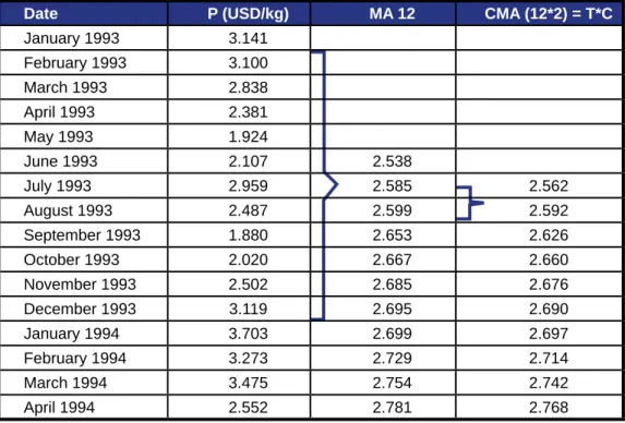
Table 2.3. Calculation of the moving average and centered moving average ...53
Table 2.4. Estimate of the trend and cycle of a time series ...55
Table 2.5. Calculation of the seasonal index and seasonality (multiplicative method) ....57
Table 2.6. Calculations using the multiplicative method...58
Table 2.7. Calculation of the seasonal index and the seasonal factor, using the additive method...62
Table 2.8. Calculations of the additive method...63
Table 3.1 Calculating the Weighted Moving Average...82
Table 3.2. Comparison of Indicators...83
Table 3.3. General Components of the CPI...85
Table 3.4. Illustration of Price Oscillator Calculation...93
Table 3.5. Calculating the RSI for Daily Coffee Prices...96
Table 3.6. Calculating the MAD and Tracking Signal for Daily Coffee Prices... ....98
Table 3.7. Calculating the MAPE ...99
Table 3.8. Illustration of an Exponential Smoothing Calculation...100
Table 3.9. Calculating the Tools for Technical Analysis of Potato Prices in USA...107
Table 3.10. Example of Exponential Smoothing...108
List of Figures
Figure 1.1. Cost, revenue and profit curve...24
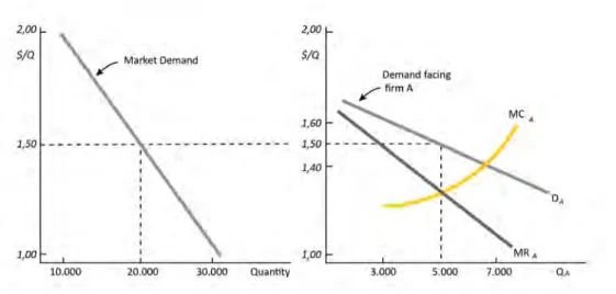
Figure 1.2. Demand curve of the farmer (a) and the market (b)...24
Figure 1.3. Cournot equilibrium...27
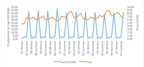
Figure 1.4. Production and price of potatoes in the United States. 1997-2007...32
Figure 1.5. U.S. potato imports and exports...33
Figure 1.6. Trend in U.S. potato stocks...33
Figure 1.7. Trend in U.S. potato productivity ...34
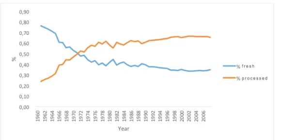
Figure 1.8. Trend in the percentage of fresh and processed potatoes consumed...35
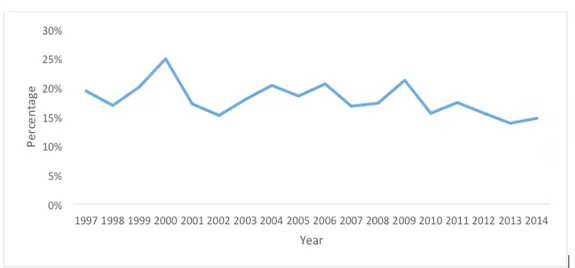
Figure 1.9. Trend in the price paid to producers as a percentage of the retail price...36
Figure 1.10. Trend in the difference between the price paid to farmers and the retail price...36
Figure 1.11. Pricing in a monopoly...37
Figure 1.12. Effect of the elasticity of the demand curve on monopoly power...38
Figure 2.1. Price of cattle at auction (USD/kg) in Costa Rica...45
Figure 2.2. Techniques for the study of time series ...50
Figure 2.3. Price behavior (USD/kg) of product x ...52
Figure 2.4. Seasonal index...56
Figure 2.5. Seasonally adjusted series and original price series...57
Figure 2.6. Volatility...58
Figure 2.7. Price of peaches (pesos/kg)...66
Figure 2.8. Seasonality of U.S. potato production (2000-2005)...66
Figure 2.9. Behavior of U.S. potato prices and the trend (2000-2005)...70
Figure 3.1. Mobile pone coverage in the districts of Kasaragod, Kannur and Kozhikode...78
Figure 3.2. Adoption of mobile phones by fishermen and prices per region...79
Figure 3.3. Bear and Bull Market Periods in USA according to S&P500...88
Figure 3.4. Orange Prices (USD/metric ton)...89
Figure 3.5. Maize Prices (USD/metric ton)...90
Figure 3.6. Long Term (12 months) and Short Term (6 months) Moving Average...91
Figure 3.7. Daily Coffee Prices and their Short and Long Term Moving Averages...92
Figure 3.8. Relative Strength Index –Daily Coffee Prices...95
Figure 3.12. Rice Prices in La Paz, Bolivia (USD/100 lbs) ...109
Figure 3.13. Banana Prices in Central America (USD/box) ...110
Figure 4.1. Evolution of Trade Agreements between Developed Countries and Developing Countries...115
Figure 4.2. Prices of Pork Producers and Wholesalers in Germany ...118
Figure 4.3. Wholesale Corn Prices in Costa Rica and International Corn Prices...120
Figure 4.4. Evolution of the Relationship between Producer and Wholesale Prices...122
Figure 4.5. Evolution of Rice Prices in China, Vietnam and USA...124
Figure 4.6. Evolution of Rice Prices in Vietnam and Colombia...125
Figure 4.7. Scale...125
Figure 4.8. Speed...126
Figure 4.9. Asymmetrical Price Transmission due to Scale ...127
Figure 4.10. Asymmetrical Price Transmission due to Speed...128
Figure 4.11. Asymmetrical Price Transmission due to Scale and Speed...128
Figure 4.12. Positive Asymmetry...129
Figure 4.13. Negative Asymmetry...130
Figure 4.14. Producers’ Price Adjustment in Reaction to Higher Wholesalers’ Prices...148
Figure 4.15. Adjustment of Producers and Wholesalers’ Prices in Case of Shock...148
Figure 4.16. Behavior of Retail Prices in Santa Cruz and Cochabamba...152
Figure 4.17. Behavior of Retail and Wholesale Prices in Santa Cruz...153
This publication is the result of a joint effort between the Market Information Organization of the Americas (MIOA), the Inter-American Institute for Cooperation on Agriculture (IICA), and the network of universities involved in the strategic actions that MIOA carries out: the Zamorano University, EARTH University, ISA University, the Luiz de Queiroz College of Agriculture of the University of São Paulo, and the University of the West Indies.
In order to identify, define, and design the technical content for each chapter in the manual, a workshop was held in July 2017 at IICA Headquarters where a number of experts and institutions contributed their guidance, knowledge, and professional experience.
The group of experts included Joaquin Arias, Specialist in Sectoral Analysis and Public Policies; Hugo Chavarria, Specialist in Sectoral Analysis; Guillermo Zuñiga, Specialist in Agricultural Business and Value Chains; Eugenia Salazar, Specialist in Sectoral Analysis; Ana Bustamante, Specialist in Virtual Learning Environments; Helena Ramirez, Coordinator of the MIOA program; Edgar Cruz, Specialist in Trade and Markets; and all personnel of the Inter-American Institute for Cooperation Agriculture (IICA). Additionally, a number of university professors and researchers provided their expertise for this manual:
Govind Seepersad of the University of the West Indies in Trinidad and Tobago; Prakash Ragbir, Manager of Information and Communication Technology at the National Agricultural Marketing and Development Corporation (NAMDEVCO); Wolfgang Baudino Pejuan Ucles of the Zamorano University in Honduras; Roger Castellon of EARTH University in Costa Rica; Anabel Then of ISA University in the Dominican Republic; Joao Gomes Martines of the Luiz de Queiroz College of Agriculture (ESALQ) in Brazil; and Victor Rodriguez Lizano and Mercedes Montero Vega, both from the University of Costa Rica.
Most of the technical content of this manual was developed based on the extensive work conducted by IICA's Center for Strategic Analysis for Agriculture (CAESPA) in this area at the hemispheric level, as part of its commitment to capacity building. The material was thoroughly examined during the workshop and later facilitated by Joaquin Arias and Hugo Chavarria for this initiative.
Mercedes Montero Vega and Víctor Rodriguez Lizano from the University of Costa Rica, and Edgar Cruz from IICA were responsible for drafting, revising, and final editing of the Manual on the Basic Analysis of Agricultural Prices for Decision-Making.
The authors would like to thank Joaquin Arias for his contribution and comments on the content of the first chapters of this manual, as well as the participants of the workshop who made observations throughout this long process.
Introduction to price analysis in
agriculture
The years 2005 to 2008 were witness to one of the biggest across-the-board increases in food prices in modern history. The price of maize more than doubled due to growing demand for biofuels, as maize is the main input used to produce ethanol in the United States. Burgeoning demand for food in emerging countries with large populations also sparked a trend toward higher maize prices (ECLAC/FAO/IICA 2012).
Furthermore, the price of wheat rose strongly during the same period, by an average rate of 28.6% per year, driven by growing demand. Some of the peaks in wheat prices were also due to lower production in Russia, Ukraine and the United States, mainly for weather- related reasons. This, in turn, resulted in unusually low inventories, largely accounting for the excessive volatility of prices during the period.
Global rice prices also increased, at an average rate of 17.5% per year. In this case, the rise was mainly due to smaller harvests in the world’s principal rice producing countries in the 2006-2007 farming year, especially in the United States, where some farmers switched to producing maize, coupled with steady growth in the demand for imports among the Asian countries, particularly Indonesia. The implementation of specific policies by countries in the region, such as Guyana’s restriction on exports, led to a reduction in global rice supplies that also contributed to the price increases.
Other events occurred that depressed food prices, however. For example, the World Bank reported that global food prices fell 14% between August 2014 and May 2015, to a five-year low. One of the main reasons for this decline was lower oil prices, which cut the cost of transportation and agrichemicals, impacting the cost structure of producers and, as a result, wholesale and retail prices (World Bank 2015).
The above examples demonstrate how prices respond to changes in economic variables and, in a simple way, how the two elements are interrelated. But, what factors determine the agricultural supply and demand? How does the market structure influence price setting? How do the basic relationships in an agricultural chain function? To answer these questions, the main objective of this chapter is to provide a holistic explanation of how prices are formed and how they serve as one of the main indicators of the operation of a market or economy.
The price of a product is affected by countless factors that are determined, to a greater or lesser degree, within the different segments of an agricultural chain. Cases will be cited throughout this chapter that demonstrate key concepts of price formation, in order to enable the reader to arrive at a better understanding of the cause and effect relationships between different variables and the price.
The chapter begins with an exploration of elements that influence price formation. Among other aspects, it describes how a price changes as its passes through the different links in the chain, and explains the concept of markup and its influence over the price observed.
This is followed by an introduction to the concepts related to the formation of the prices of products traded internationally. This distinction is made given the particular complexity of price formation in the case of imported and exported products.
Three other aspects are then addressed. An analysis of the determinants of supply and demand is followed by examples of price setting under different market structures. The way in which prices vary in response to changes in their determinants is then explained, in order to introduce the concept of elasticity.
1.1 An initial overview of price formation
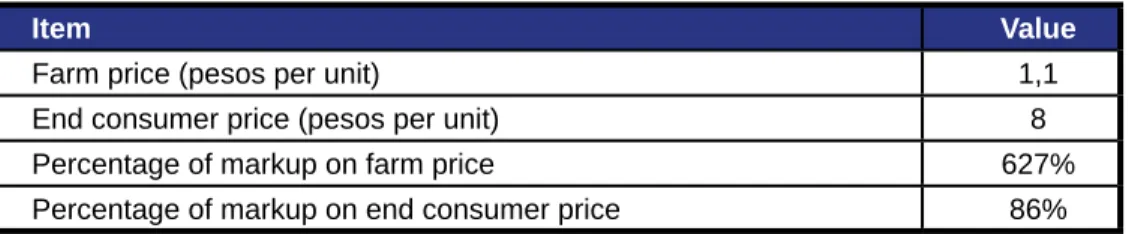
Thus far, the word “price” has been used in a general sense, without alluding to a specific link in the production chain. In fact, it is possible to identify various prices at different points in the chain. The mostly widely disseminated time series are those dealing with farm, wholesale and retail prices, so when speaking about prices it is important to consider the point in the chain involved. For example, in 2014 the farm price of limes in Mexico was 1.1 pesos but the end consumer price was 8 pesos per unit (Chavez 2014). The reason for this has to do with the concept of markup in agricultural chains. Middlemen purchase a product lower down the chain and resell it at a higher price further along. In the case of limes, the percentage of markup between the price paid to the producer and the price paid by the end consumer was 86% (Table 1.1).
Table 1.1. Lime prices and percentage of markup in pesos in Mexico.
Item Value
Farm price (pesos per unit) 1,1
End consumer price (pesos per unit) 8
Percentage of markup on farm price 627%
Percentage of markup on end consumer price 86%
Source: prepared based on Chavez 2014.
In Zarcero, Costa Rica, a producer estimates that the cost of producing a bunch of cilantro is roughly 95.73 colones. To obtain a 25%
return on her investment, she needs to sell each bunch for around 120 colones.
An intermediary pays the farmer 120 colones per bunch, but then incurs a series of costs, such as freight, travel, loading and unloading, and other expenses. If the intermediary aims to sell the bunches of cilantro to a retailer in the local markets held weekly, he will have to take into account the 120 colones paid for each bunch, plus markup costs and a percentage of profit. If the markup costs total 20 colones per bunch, the intermediary would so far have invested 140 colones per bunch of cilantro.
If the intermediary aims to make a 50% profit on his investment, he will sell each bunch to the retail seller for 210 colones (140 x 1.5). The retailer purchases each bunch of cilantro for 210 colones, but must factor in right of sale and other costs incurred in running a market pitch. Thus, the retail seller estimates his expenditure to be 20 colones per bunch of cilantro. If the retailer wishes to obtain a 30% return on his investment, he will need to sell each bunch of cilantro to the end consumer for roughly 300 colones (230 x 1.3).
It should be noted that the markup margin, in this case 6.9 pesos (8-1.1), does not represent the profit made by the intermediary, since transaction, costs are incurred when a product passes along the agricultural chain, from one link to another. The main expenses incurred by the intermediary are transaction, transportation and refrigeration costs.
Consider the following case, which highlights the importance of these costs in the formation of the final price of a product.
A case of domestic price formation in Costa Rica
The above example provides a general explanation of price formation throughout a chain; however, there are distinctive features in the countries that also influence the price formation process throughout the chain. To gain a better understanding of this process, a study was carried out to examine the behavior of agricultural prices in Latin America, focusing on the price formation process of 54 agricultural products in 12 regions. The factors that have an important impact on prices were found to include the regions’ agricultural structures, the conditions for accessing them, and the technologies used to grow crops.
One of the main conclusions of the study was that price formation depended intrinsically on the characteristics of the different regions and products. Broadly speaking, it is important to consider:
PRODUCER Sale price
(95,73)
INTERMEDIARY Sale price
(210)
RETAIL SELLER Sale price
(300)
Markup margin 90 colones
Markup margin 114,27 colones
A summary of the process is shown in the following diagram:
• farm structure
• the level of diversification of farm production and the existence of local markets
• domestic freight costs
• links with other regions
• access to information
• the prices of agricultural inputs (which account for 20%-60% of the total costs of the factors of production). However, these also depend on the prices of the technology available (IICA 2014).
Given the major differences that can exist among the aforementioned factors, it is necessary to conduct a specific analysis in each region, even within each country or territory. For example, a study of this kind carried out in Peru focused on three regions with three different types of territories (the coastal, highland and rainforest regions) and differences with regard to the use of technology, access to water, target markets and ease of transportation, factors that have a major impact on the selection of crops and the return on production. The data for the three regions gives an overview of the behavior of price formation in accordance with the characteristics of each one (Paz-Cafferata 2010).
The example cited above explains the price formation process of an item produced and sold within a country; however, Latin America and the Caribbean’s agricultural balance of trade has historically been positive (a trade surplus), which means that, in economic terms, the region exports more than it imports.
Given the major contribution that the region makes to international agricultural trade, it is especially important to understand the price formation process of products that are traded internationally. The price at which an imported product is sold can be influenced by variables other than the ones that impact the price of a good produced and sold within the country, since the marketing chain tends to be less complex in local markets. International markets, on the other hand, involve a greater number of players, leading to higher costs when the payment of tariffs, licenses, permits, etc., has been factored in.
Some of the most important variables related to transportation that affect the price of an imported product are the following costs:
1. Freight 2. Insurance 3. Lost product 4. Storage
5. Import and export duties
For an in-depth analysis of these and other variables, and of the concept of Incoterms, see Frank (2006).
The following example shows some of the costs that have to be taken into account when an agricultural product is exported or imported, as they play a key role in the price formation of such products.
An exporter needs to ship a container full of agricultural product “x”, having agreed to deliver it on board a ship in the final port of destination.
This means the exporter will have to defray the cost of road freight from the plant to the port of shipment, and then the cost of sea freight to the port of destination.
To calculate the costs of this operation, one of the first variables that must be taken into account is the distance, as well as the container’s size (20’ or 40’ – 1 or 2 TEU) and type (dry, refrigerated or frozen).
The following illustrative, but not exhaustive list, shows some of the pertinent costs:
The shipping and export and import costs would amount to USD 2150, broken down as follows:
• Road freight to port: 110 • Sea freight: 1120
• Documentation, destination 50 • Disembarkation, destination 150 • Documentation, place of origin 65
• Export from Veracruz (border/port compliance): 400 • Export documentation 60
• Importation into Acajutla (border/port compliance): 128 • Import documentation: 67
Assuming that roughly 1400 boxes fit into a container of this kind, the cost per box would be USD 1.54.
The above is an estimate of the real cost, calculated using the IDB’s transport cost estimator tool (IDB 2017). Numerous trade agreements between countries currently exist that establish tariff conditions for specific products, so this aspect must be taken into account within the price formation process of products traded on the international market.
Price formation process in the case of imports
As has been shown, the agriculture sector is highly complex and has prices that serve as market “thermometers,” reflecting not only a product’s relative abundance or scarcity, but also the trends in other variables. One thing that all the aforementioned variables have in common is that they affect the supply or the demand, either directly or indirectly. Therefore, the next step is to analyze the determinants of the supply and demand in an agricultural market, in order to gain a better understanding of price formation in agriculture.
1.2 Determinants of supply and demand
The price of an agricultural product is determined mainly by the interaction between the supply and the demand, which are influenced by a series of factors.
The determinants of the supply and demand for agricultural products that influence price behavior are analyzed in the following sections. For example, the agronomic requirements of some crops mean that they can only be harvested at certain times, so that supplies vary over the course of the year. These changes in the supply lead to variations in prices, which follow a similar pattern every year.
1.2.1 Price determinants of supply
In the case of the agriculture sector, the supply may include not only fresh produce and/
or processed products but also agricultural inputs and machinery, technical assistance, agricultural loans and land, and many other elements. Given the highly complex and wide- ranging nature of the subject, this section will only address the supply of fresh produce, under the premise that the main generator of the supply are producers and certain variables that they do not control but which directly affect their production decisions and yields. The following example is by way of an introduction to the concept of supply.
In 2008, the six fruits that accounted for the lion’s share of fruit production in the United States were, in descending order of importance, grapes (an estimated 22.3%), apples (14.0%), strawberries (11.3%), cherries (4.0%), cranberries (3.9%), peaches (3.3%) and pears (2.3%).
It is worth noting that the above percentages can vary from year to year due to changes in market conditions. In 2006, the grape harvest declined by approximately 8.3%, due to adverse climatic conditions in California, which was one of the main reasons why prices were higher than in 2005. On the other hand, strawberry and cherry production increased during 2007, by 14.8% and 25.5% respectively. Weather patterns and changes in agricultural support policies have driven the increase in fruit production in Canada (24.6%) and the European Union (7.3%) over the last five years. An important point to bear in mind is that U.S. supplies of strawberries can no longer keep up with demand for the fruit in the winter months, due to labor costs.
Domestic production supplies the U.S. fresh strawberry market but, in addition to being the world’s largest producer, the country is the leading consumer (more than one million tons per year). Most domestic supplies (nearly 90%) are produced in California. However, in Canada the supply of domestic strawberries is weaker, so that most of the fruit is imported.
The above data was taken from a SAGARPA study carried out in 2009 to garner information about the supply of fruit, especially strawberries, in the United States and Canada with a view to identifying market opportunities. As can be seen from this case study, domestic supplies of a product can be affected by the phenological state of plantations, climatic events, import and export levels, support policies, labor costs, the price of the product, and other variables that will be addressed in greater depth in this module.
Source: prepared based on SAGARPA 2009.
Understanding supply
There is a direct causal relationship between the quantity of a product that is available and its price: the higher the price, the bigger the supply, as rising prices are an incentive for producers to sell more produce.
Unlike its industrial counterpart, agricultural production depends on the production cycles of plants and animals, which means that one of the biggest limitations to the supply of agricultural products is the availability of products for immediate marketing, since they may have been planted but are not ripe enough to be of interest to the market. More produce is available around harvest times and prices are usually low. On the other hand, when production is low, little product is available and prices are high. Unlike other sectors, the production cycle of crops is one of the determinants, since detailed planning is required to be able to supply a product on a specific date.
It is important to remember that agricultural products have different types of cycles and can be divided into:
1. Short-cycle crops 2. Semi-permanent crops 3. Perennial crops
Farmers who are familiar with the cycle of a given product will have access to information about harvest cycles and forecasts, and be able to:
• Program the marketing of agricultural products according to the demand • Predict the qualities of an agricultural product
• Identify production areas
• Identify markets for each product
Where:
P= price of the product Q= quantity
Pinp= price of inputs (seeds, fertilizers, labor, etc.) T= technology
Cl= climate, pests and diseases
Pc= price of products competing for the same
resources
Pa= prices of associated crops R= existing inventories, stocks, reserves
N= number of hectares (area) or production structure of crops G= government policies
Exp= expectations and attitudes of producers
According to the law of supply, an increase in the price of an agricultural product results in an increase in the quantity supplied. When the price drops, the opposite occurs. This phenomenon is closely linked to producers’ expectations and attitudes. For example, small-scale and low-income producers tend to be more risk averse, so they reduce or cease production when faced with a drop in prices or climate risks.
If the price of a product has been rising during recent production cycles, more producers are likely to produce that good, thus increasing the number of hectares planted with the crop and, as a result, the supply. In this regard, it should be borne in mind that failure to control the production of a good usually results in an oversupply, mainly during peak harvest times, which instead depresses prices.
A case in point was what occurred with sugarcane between 2011 and April 2013. During that period, sugar production responded to the stimulus of the good prices paid in previous years, resulting in significantly higher sugarcane harvests in key producer countries like In addition to the cycle, several other factors affect the supply and, consequently, the price of a crop. The price of an agricultural product can therefore be expressed as a function of different variables:
P=f(Q,Pinp,T,Cl,Pc,Pa,R,N,G,Exp)
(marketing, state intervention, plant health standards, legal problems with land tenure)
Brazil, Thailand, Australia and Mexico, and a global sugar surplus. Over that period, the price of sugar was 30.1% below the long-term trend, mainly because of the oversupply.
China also reduced its overseas purchases of sugar due to larger domestic supplies, which shows how stocks or inventories also play an important role in price formation (IICA 2014).
Another price determinant is the technology available for production, as the higher the technological level, the more efficient the production system. Efficiency translates into the use of fewer inputs per unit. Thus, to a large extent, the agricultural supply depends on the development and adoption of technology.
In the case of Mexico, and the Puebla region specifically, the timely implementation of recommended technology made it possible to achieve experimental yields of up to five, seven and eight tons of maize per hectare (Aceves et al. 1993). However, the National Institute of Statistics and Geography reported that over the period 1993-2004, the yield was 2.6 tons per hectare (INEGI 2007), and 2.54 tons per hectare in 2008 (SIAP 2009).
According to Osorio-García et al. (2012), the failure to adopt the technology generated was the main reason for this low productivity.
Climatological factors, pests and diseases determine the availability of the supply of agricultural products. For example, between 2011 and 2013 the international price of coffee rose by an average of 36%, due to outbreaks of rust in Central America, Colombia and Peru that reduced the supply and drove up the price. During the same period, the United States suffered the worst droughts in its history, resulting in higher international maize prices and a 30.6% deviation from the long-term trend (IICA 2014).
The existence of other products that compete for the same resources is another price determinant. It should be remembered that land, labor and capital are the principal factors of production. The supply of crop A in a given area can be affected by the introduction of another crop (B) that also requires labor, land or capital. Thus, the larger the number of hectares planted with crop B, the smaller the quantity of factors of production available for crop A, and the smaller the supply.
The way in which information about the level of inventories is managed can cause sharp changes in agricultural prices in the short term. One study carried out in the region suggests that incomplete information on the availability of inventories can trigger abrupt changes in prices, and also explains that good inventory management is regarded as part of risk management. Hence, price volatility is less of a problem in economies that have sound inventory management policies, and such countries are less vulnerable to the vagaries of the international market.
This shows how sensitive prices can be to inventory levels. It is also suggested that storable (non-perishable) products are subject to less price volatility than perishable ones whose inventories are kept to a minimum (ECLAC/FAO/IICA 2011).
Another determinant of the supply of a product is state intervention. For example, in Costa Rica the price of rice is regulated throughout the chain. Such regulation makes for greater price stability, but the price of rice does not necessarily respond efficiently to scenarios in which production is small or input costs increase. This can be a disincentive for producers when they come to sell the product, since the price may not reflect the true cost of producing the rice or the true supply situation. For more in-depth information about the system used to regulate the price of rice in Costa Rica, see León-Sáenz and Arroyo- Blanco (2011).
Por último, es de importancia entender que existen factores que afectan el coFinally, it is important to bear in mind that there are factors that affect the behavior of prices in the short, medium and long run. This makes it easier to understand the behavior of prices, since it provides information that makes it possible to differentiate between temporary or short-term factors and structural ones, both of which affect the behavior of the price.
A short-term factor refers to the behavior of economic variables, given specific natural or market situations that arise and temporarily affect variations in the production and consumption of agricultural goods. (Salinas-Callejas 2016). Political decisions are usually a response to temporary situations, as in most cases they are designed to stabilize prices after an event of some kind has occurred. Examples of temporary situations are droughts or the appearance of a pest that causes major production losses.
Structural changes, on the other hand, explain the behavior of prices in the medium and long terms (the trend). For example, technological innovation, higher productivity, lower costs, variations in cultivated area and changes in the alternative uses of agricultural goods are some of the variables that can be classed as structural. This means they have a permanent effect on variations in the production and consumption of agricultural goods, as long as the conditions persist.
1.2.2 Price determinants of demand
Consumption decisions are influenced by a series of factors that are known as determinants of demand. Consumption patterns can vary depending on consumer tastes and preferences, product perishability, and the evolution of consumer income over time as it shapes consumption. It should be noted that these factors affect the demand, and also influence the price.
For example, there are documented accounts of vegetable growing and consumption dating back to 8000 B.C., when mainly peas, beans and lentils were consumed. While these crops continue to be key in combating malnutrition, reducing poverty and contributing to human health, the evolution of vegetables has been very different from the increase in the production and consumption of other crops such as maize, wheat and rice. Since the Green Revolution (around the 1960s), all these products have seen production increases Related concept: price
elasticity of supply As has been discussed
in this section, there is an important relationship between the price and the quantity supplied of a good. It is due to the importance of this relationship that the concept of elasticity is introduced, which indicates the responsiveness of the quantity supplied to changes in prices.
As is to be expected, higher prices stimulate production, which means that a positive relationship is maintained between the price and the quantity supplied. For example, if the elasticity of supply is 1.3, it means that if the price changes by one percent, the quantity supplied will change by 1.3%.
of between 200% and 800%, while vegetable production has grown by only 59%. In this regard, production and consumption decisions are interconnected; producers grow crops for which they are certain there will be most demand, and it is in order to understand these consumption patterns that the determinants of demand are analyzed (FAO 2016).
Agricultural prices are influenced by variables that influence demand for the product.
The main variables are shown below:
Where:
P= price of the product Q= quantity
I= income of consumers TP= tastes and preferences of consumers
G= government policies (sales tax,subsidies)
Pe= perishability of the products Ss= socioenvironmental
specifications
Pr= prices of related
P=f( Q,I,TP,G,Pe,Ss,Pr )
(complementary and substitute) products
Both developed and developing countries continue to increase their consumption of maize, wheat, rice, dairy products and meat; however, no changes are foreseen in the pattern of vegetable consumption, which is expected to remain at 7 kg per person per year.
This pattern is due to both consumer tastes and preferences and consumer income. It has been observed that as income rises, consumer diets change: the population consumes fewer plant proteins and more expensive proteins, such as dairy products and meat. Thus, the greater the purchasing power, the smaller the proportional consumption of vegetables (certain types of food replace others). Products of this kind, whose consumption decreases when consumer income increases, are known as inferior goods.
There is another type of product (e.g., organic and fresh products, products with fair trade seals or some other kind of guarantee) that offer consumers greater value added and, as such, reflect a positive relationship between consumption and consumer purchasing power. In the search for a healthier lifestyle, consumption of organic products has been increasing at around two to three percent worldwide. This leads to changes in production systems that are the result of pressure from consumers who have opted for foodstuffs that do not contain chemicals, contributing not only to human health but also to a reduction in
agricultural production’s impact on natural resources. For example, although no official figures on the performance of the country’s organic market are available, the Organic Agriculture Group of Chile estimates that the domestic organic market generates around USD 35 million per year. It is a new market enjoying 20% annual growth, even though organic products usually cost about 25% more than products grown and harvested using conventional agricultural methods (USDA 2010).
Food consumption has increased across the globe as consumer incomes have risen more than prices. In regions with developing countries, food consumption has increased considerably, especially if there have been substantial increases in income. However, in Sub-Saharan Africa, higher agricultural prices meant that food consumption in 2012 was 11% lower than in 2000, despite a population increase of 38% over the same period (World Bank 2017). In both Europe and North America, on the other hand, food consumption has remained constant, because consumers with sustained high incomes are not going to increase their food consumption in the same proportion as changes in their income, since food is a basic need that is already covered (FAO 2012).
In the two cases mentioned above, the patterns of behavior of both vegetables and organic products reflect tastes and preferences, as well as consumer incomes, which are some of the price determinants.
As most agricultural products are perishable, they need to be bought and sold within a short period of time. Unlike other products, in most cases farmers and merchants cannot store them, especially if fresh produce is involved. Consumer tastes and preferences are one of the variables that must be considered when studying price formation. Although one refers to agricultural products in general, there are significant differences between fresh produce and storable products, which have a much longer shelf life.
One problem with vegetables, for example, is that they must be consumed within a very short period of time, as many are consumed fresh. As much as 45% of global fruit and vegetable production is wasted. Fruits and vegetables are the group of products with the highest wastage rate, and their short shelf life is the main reason (FAO 2012).
Products with a distinctive seal are a clear example of how the demand for products varies according to consumer tastes, preferences and income. In this regard, all quality seals, such as certifications of organic products like Fairtrade and Global Gap, are designed to demonstrate that products meet a series of specifications for which the consumer is willing to pay. This type of consumer is willing to pay a premium price to ensure that the products are of a higher quality or meet socioenvironmental specifications in the production systems within which they are produced. The quality of a product depends on the elements that are regarded as defining that quality. The market establishes quality based on the value that consumers assign to a product, linked to a set of properties or characteristics they rate or perceive as being superior to the other products in the market (Arvelo et al. 2016).
Like the organic products mentioned previously, the consumption of certified products has also been on the rise in recent years, reflecting the demand in some niche markets.
Global consumption of Fairtrade certified coffee is a case in point. Six percent more volume was produced in 2013-2014, with the total reaching 150,800 metric tons (Fairtrade 2015).
The production and marketing of certified cacao has also grown considerably, mainly due to the chocolate industry’s responsiveness to the demands of consumers. In 2012, 150,000 tons of cacao were produced with the Fairtrade seal, 98,400 tons with the Rainforest Alliance label, 214,000 tons certified by the UTZ program and 45,000 tons with the organic seal (Arvelo et al. 2016). However, these consumption trends are heavily dependent on consumer incomes and, as already mentioned, on the market niches in which the product is sold.
Adopting a similar approach to the one employed for the section on supply, we shall now turn to the concept of elasticity of demand.
Concept of elasticity of demand:
Spending on food makes up only a small part of the total budget of high-income consumers, such as those in the OECD countries. As a result, consumers of this kind are relatively indifferent to even quite sharp fluctuations in agricultural prices. This relationship between the change in the quantity consumed and price swings is known as the price elasticity of demand.
In economic terms, this kind of consumer is more inelastic1 with respect to prices than poor consumers living in developing countries, who purchase mostly basic foodstuffs with less value added. This means that the prices of basic agricultural products account for a bigger proportion of the final price they pay for food, and food is an important part of household expenditure (CFS 2011).
In addition to variations in prices, changes in income are another factor that may lead consumers to alter their consumption patterns. This relationship is known as income elasticity of demand. Consider the following example, which contains an analysis of changes in milk consumption in the Central American countries related to income and cheese prices.
1Inelastic behavior is the term used to describe a situation in which the proportional change in income is bigger than the proportional change in food consumption.
In 2012, a study was conducted to analyze the behavior of fluid milk and cheese consumption in Central America, with a view to identifying the consequences of the entry into force of the Free Trade Agreement between Central America and the United States. Some of the results of this study are shown in the following table. With respect to price elasticity, it suggests that a one percent change in the price of cheese leads to a change in consumption of 0.212% in Costa Rica, -0.937% in El Salvador, 0.233% in Guatemala, 0.564% in Honduras and 0.591% in Nicaragua. Consumption falls as the price of cheese increases but the proportional change is less than one percent; because of this, cheese is regarded as an inelastic good.
Price elasticity is negative in all of the countries except Costa Rica, suggesting that as the prices of products rise, consumption will fall. The behavior with regard to income elasticity indicates that the higher the income, the greater the consumption
Variable Costa Rica
El Salvador
Guatemala Honduras Nicaragua
Price elasticity
0,212 -0,937 -0,233 -0,564 -0,591
Income elasticity
0,150 1,204 0,309 0,715 0,417
The above table shows that El Salvador’s elasticity is greater than that of the other countries: consumption declines by 0.937% in response to a one percent increase in the price, while the figure for Guatemala is only 0.233%. Analyzing the behavior of income elasticity, cheese consumption in El Salvador rises 1.204% in response to a one percent change in income, while in Costa Rica the figure would be only 0.15%.
The level of consumer income is one of the determinants of demand.
In the case of foodstuffs, the higher the income level, the greater the
Price elasticity and income elasticity:
cheese in Central America
inelasticity of demand, in terms of both price elasticity and income elasticity. For example, in the European Union the price elasticity of cheese is -0.18 and income elasticity is 0.03 (FAPRI 2017), which means that when there are changes in the price, consumption will remain much more constant than in Central America.
Estimating price elasticity and income elasticity is useful for predicting how a market is going to react to changes in these variables, thus making it possible to anticipate the socioeconomic changes that such variations in consumption can trigger.
Source: prepared based on Huang and Durón-Benítez 2015.
The diets of all human beings are formed of combinations of agricultural products;
however, the combination of foodstuffs is linked to the prices of products, and to the other determinants of demand. As a result, the price of a product is also determined by the prices of related products, whether substitutes or complementary products. If two products complement one another, they are referred to as complements. In this case, if the price of one good increases, consumption of the other is going to fall, since they are consumed together.
If, on the other hand, two products are substitutable, they are known as substitute products. In this case, if the price of one good increases, an increase in the consumption of the other is to be expected, as consumers begin replacing one with the other. The concept of cross elasticity is used to analyze the relationship between related goods;
that is, the behavior of consumption of one good (A) in response to changes in the price of another good (B).
Data on the consumption and prices of black tea and coffee in the United States was analyzed to determine the behavior of the consumption of both between 1990 and 2008. According to the price elasticity of tea, tea is an inelastic good, while coffee is elastic. This means that if prices begin to fall, coffee consumption is going to replace tea consumption. As coffee is a more elastic product, when prices fall there will be a bigger increase in the quantity demanded and, therefore, in consumption. Assuming that the size of the market remains constant, people are going to consume more coffee in place of tea.
Cross elasticity: substitute products and complements
Variable Black tea Coffee
Black tea -0,393 0,125
Coffee 0,599 -1,022
Income elasticity 0,837 1,008
Source: adapted from FAO 2011.
In the case of complements, an analysis of consumption habits related to groups of products in Japan estimated that the cross elasticity between rice and oil is –0.228, meaning that when the price of one of these goods increases, consumption of the other decreases.
This situation occurs because if the price increases and consumers eat less rice, consumption of the oils used to cook it also decreases (FAO 2003).
In the case of both the vegetables and organic products already mentioned, such movements in the demand curve cannot necessarily be adjusted by means of local production, since the rate of growth of the total population is greater than the rate of agricultural production. As a result, in many cases countries are forced to import these products, thereby increasing the volume of international agricultural trade. All these changes in consumption patterns are directly related to the price formation process of the agricultural products that are the main focus of study in this manual.
Another element that has a major impact on price formation is the structure of the market in which a good is traded. The various dimensions of this subject are worth analyzing separately, so the way in which market structures influence the formation of agricultural prices will be addressed in the next section.
1.3 Market structures and price formation
As explained in the previous section, the price formation process is influenced by a series of national and international variables. The latter include trade liberalization, the size of the economy, the degree of self-sufficiency and tariffs, quotas and other trade barriers. For example, the extent to which the domestic price of a product is influenced or determined by the international price is directly dependent on trade liberalization.
Market structures also influence price formation. Therefore, this section focuses on the influence of market structures in determining agricultural prices.
1.3.1 Perfect competition
A market is competitive when there are many buyers and many sellers, and the product traded is homogeneous. Precisely because firms have little market power, none of them can influence pricing on their own. Since one of the assumptions of perfect competition is product homogeneity, the differentiation of products is one of the reasons why conditions of perfect competition are rarely seen. Even in the case of the agriculture sector and fresh produce, certain differentiation exists in terms of quality. Markets fulfill most of the assumptions of perfect competition, however, as there are a large number of suppliers of fairly homogeneous products and both producers and consumers have access to price information.
Agricultural markets are designed to enable buyers to have direct contact with farmers, and are a commonly used mechanism for buying and selling, especially in the case of fresh produce. For example, agricultural and farmers’ markets have long existed in Argentina but in the mid-1990s farmers engaged with rural development organizations in the province of Misiones to establish family farmers’ markets, or ferias francas. A typical feria has an average of 12 pitches, with around 20 families involved. However, a very wide variety of products is sold and the number of pitches varies from 3 to 120, depending on the market concerned (Goldberg 2010).
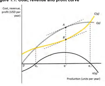
In markets, all farmers try to maximize profits and this occurs when the difference between producers’ revenue and costs is the maximum, as can be observed in the following figure (Figure 1.1). The maximum distance is observed when the distance between total income and total costs is the greatest; that is, the distance between A and B.