HAL Id: insu-02512853
https://hal-insu.archives-ouvertes.fr/insu-02512853
Submitted on 20 Mar 2020
HAL is a multi-disciplinary open access
archive for the deposit and dissemination of
sci-entific research documents, whether they are
pub-lished or not. The documents may come from
teaching and research institutions in France or
abroad, or from public or private research centers.
L’archive ouverte pluridisciplinaire HAL, est
destinée au dépôt et à la diffusion de documents
scientifiques de niveau recherche, publiés ou non,
émanant des établissements d’enseignement et de
recherche français ou étrangers, des laboratoires
publics ou privés.
Distributed under a Creative Commons Attribution - NonCommercial| 4.0 International
Comparisons of simulations with microfluidic
experiments
Filip Dutka, Vitaliy Starchenko, Florian Osselin, Silvana Magni, Piotr
Szymczak, Anthony J.C. Ladd
To cite this version:
Filip Dutka, Vitaliy Starchenko, Florian Osselin, Silvana Magni, Piotr Szymczak, et al..
Time-dependent shapes of a dissolving mineral grain: Comparisons of simulations with microfluidic
exper-iments. Chemical Geology, Elsevier, 2020, 540, pp.119459. �10.1016/j.chemgeo.2019.119459�.
�insu-02512853�
Contents lists available atScienceDirect
Chemical Geology
journal homepage:www.elsevier.com/locate/chemgeo
Time-dependent shapes of a dissolving mineral grain: Comparisons of
simulations with microfluidic experiments
Filip Dutka
a, Vitaliy Starchenko
b, Florian Osselin
c, Silvana Magni
a,e, Piotr Szymczak
a,∗
,
Anthony J.C. Ladd
d,∗
aInstitute of Theoretical Physics, Faculty of Physics, University of Warsaw, Pasteura 5, Warsaw 02-093, Poland bChemical Sciences Division, Oak Ridge National Laboratory, Oak Ridge, TN 37830, USA
cInstitut des Sciences de la Terre d’Orléans, 1A rue de la Férollerie - 45100 Orléans, France dDepartment of Chemical Engineering, University of Florida, Gainesville, FL, USA
eInstitute of Geophysics, Polish Academy of Sciences, Ksiecia Janusza 64, 01-452 Warsaw, Poland
A R T I C L E I N F O
Editor: Karen Johannesson
Keywords:
Pore scale modeling Gypsum dissolution Dissolution rate Simulation and experiment Reactive surface area
A B S T R A C T
Experimental observations of the dissolution of calcium sulfate by flowing water have been used to investigate the assumptions underlying pore-scale models of reactive transport. Microfluidic experiments were designed to observe changes in size and shape as cylindrical disks (radius 10 mm) of gypsum dissolved for periods of up to 40 days. The dissolution flux over the whole surface of the sample can be determined by observing the motion of the interface. However, in order to extract surface reaction rates, numerical simulations are required to account for diffusional hindrance across the concentration boundary layer; the geometry is too complex for analytic solutions.
We have found that a first-principles simulation of pore-scale flow and transport, with a single value of the surface reaction rate, was able to reproduce the time sequence of sample shapes without any fitting parameters. The value of the rate constant is close to recent experimental measurements but much smaller than some earlier values. The shape evolution is a more stringent test of the validity of the method than average measurements such as effluent concentration, because it requires the correct flux at each point on the sample surface.
1. Introduction
Mineral dissolution (and precipitation) reactions involve mass transfer over a wide range of scales. Chemical bond breaking and sol-vation of the resulting ions occurs on scales below 1 nm. However, in the absence of ion transport, fluid in the neighborhood of the mineral surface will become saturated and dissolution will cease. The volume taken up by the solution containing the dissolved ions is typically three to six orders of magnitude larger than the volume of mineral from which they originated. For example, a limestone dissolution front ad-vancing 1 cm would need to distribute the dissolved calcium ions over a distance of about 100 m for the solution to remain below saturation. Ion advection is therefore essential for large scale changes in mineral composition; diffusional processes alone cannot operate over these scales in a realistic time frame. Laboratory experiments often seek to minimize transport hindrance by inducing advection, for instance with a spinning disk or stirred batch reactor. However, analysis of transport hindrance is not straightforward; in some cases it is the primary cause
of variability in published rate constants (Colombani, 2008). Since gypsum dissolves fairly rapidly, even in pure water, some degree of transport control of the dissolution kinetics is to be expected.
Reactive surface area underpins the use of chemical rate coefficients in Darcy-scale models of reactive transport (Steefel et al., 2014). In principle, it reflects the number of active reaction sites on the mineral surface and can be estimated from a BET absorption isotherm (Colón et al., 2004; Hodson, 2006) or from X-ray tomography measurements of the accessible pore space (Landrot et al., 2012; Noiriel et al., 2009). Both methods allow rate constant measurements to be correlated among related experimental methods (Rimstidt et al., 2012), but in the absence of an understanding of the pore-scale flow paths, the inhibiting effects of ion transport on mineral dissolution rate cannot be estab-lished with any degree of reliability. In minerals that are very slow to dissolve, for example quartz, dissolution may be entirely controlled by the surface reaction rate, but more commonly the kinetics are mixed, with both surface reactions and ion transport hindering the mass transfer across the mineral-fluid interface. This means that measured
https://doi.org/10.1016/j.chemgeo.2019.119459
Received 20 August 2019; Received in revised form 18 December 2019; Accepted 31 December 2019
∗Corresponding authors.
E-mail addresses:[email protected](P. Szymczak),[email protected](A.J.C. Ladd).
Available online 07 January 2020
0009-2541/ © 2020 The Authors. Published by Elsevier B.V. This is an open access article under the CC BY-NC-ND license (http://creativecommons.org/licenses/by-nc-nd/4.0/).
dissolution rates are dependent on the experimental setup, and further analysis is needed to extract consistent surface reaction rates (Colombani, 2008; Colombani and Bert, 2007). However, analytical analysis depends on simplified models of mass transfer from the surface to the bulk and cannot account for new flow paths created by an evolving pore space (Upadhyay et al., 2015).
Pore scale numerical simulations are a means by which rates of mass transfer to and from a dissolving boundary can be accurately calculated based on molecular-scale parameters. Resolving the flow and ion transport within the pore space (De Baere et al., 2016; Molins et al., 2012, 2014; Oliveira et al., 2019; Starchenko et al., 2016) can avoid the uncertainties inherent in Darcy-scale modeling, by using only in-dependently measurable properties as input: surface reaction rates, ion activities, diffusion coefficients, and equilibrium constants. Such models can provide detailed information on the spatial distribution of reaction rates across the mineral surface, not just average properties such as effluent flux. However, the spatial distribution of the con-centration in a reactive system is difficult to measure experimentally, making a detailed validation of a pore-scale model problematic. Nevertheless, microfluidic experiments offer the opportunity to explore local dissolution rates, via frequent optical imaging of a dissolving mineral surface (Osselin et al., 2016; Soulaine et al., 2017). The evol-ving shapes of the mineral-fluid boundary represent a direct measure-ment of the local dissolution rate. Our interest here is to discover to what extent a pore-scale model can predict the outcome of microfluidic experiments when the parameters in the model can be tightly bound by independent measurements.
In this paper we make a stringent test of the validity of the equations for pore-scale reactive transport, by comparing high resolution nu-merical simulations of a dissolving grain with microfluidic experiments. We focus on gypsum (CaSO4⋅2H2O) as a model geochemical system,
because of its simple dissolution pathway in water,
CaSO4⋅2H2O(s) → Ca2++ SO42−+ 2 H2O, (1)
and because samples can be prepared in a variety of shapes by rehy-drating the powdered hemihydrate (CaSO4⋅12H2O). Gypsum dissolution
involves both a kinetically controlled rate and a speciation reaction, Ca2++ SO
42−↔ CaSO4(aq); (2)
near saturation approximately one-third of the dissolved calcium is in the aqueous CaSO4complex. Despite the simple chemistry, the system
encompasses the key features of reactive transport in porous media:
fluid flow, reactive transport of aqueous ions, kinetic and equilibrium reactions, and an evolving pore space. Nevertheless the pore-scale equations contain only a few parameters, all of which can be de-termined independently.
2. Methods
An integrated set of experiments and numerical simulations have been designed to probe the capability of reactive transport models to capture local dissolution fluxes at mineral-fluid interfaces. We are in-terested to see if a reactive transport model can capture both the overall dissolution rate, as measured by the change in volume of the soluble mineral, and the distribution of reactive flux over the mineral surface, as measured by changes in shape. To that end we have modified a microfluidic cell (Osselin et al., 2016), which allows for visual imaging of a gypsum disk as it dissolves in flowing water. The experiment was simulated using the equations of reactive transport: fluid flow, ion ad-vection/diffusion and chemical reactions at the mineral-fluid interface. The unstructured mesh conforms to the location of the interface, which allows for precise calculation of the reactive fluxes. Mesh points on the mineral-fluid interface move in response to the local dissolution flux, while overall mesh quality is preserved by Laplacian smoothing. 2.1. Experimental methods
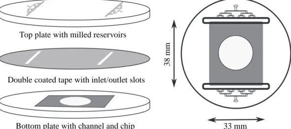
The microfluidic cell was modified from the design reported in Osselin et al. (2016). It consists of two circular plates 65 mm in dia-meter and 10 mm thickness made of MakroclearⓇ polycarbonate
(Fig. 1). The bottom plate contains a rectangular indentation (38 mm × 33 mm × 0.5 mm), which was engraved using an MSG4025 CNC micro milling machine (Ergwind, Gdansk). The top plate, engraved by the same machine, contains milled channels which conduct water to the Hele-Shaw cell formed by the plates. A hierarchical cascade of channels connects to large reservoirs in the top plate (45 mm × 5 mm × 2 mm), which assists in distributing the pressure uniformly across the inlet and outlet of the Hele-Shaw cell.
A cylindrical gypsum disk, radius a = 10 mm and height h = 0.5 mm is attached to the base of the cell, in the center of the 38 mm × 33 mm channel. The disk is prepared by inserting a plastic mold with a circular hole into the indentation in the bottom plate (Fig. 1). The plaster solution is then poured into the mold and compressed for 30 min under a light mechanical load, dried for 24 h and polished by sandpaper (500 grit). The plates (top and bottom) are sealed using ultra-thin
Bottom plate with channel and chip
Double coated tape with inlet/outlet slots
Top plate with milled reservoirs
33 mm
38 mm
Fig. 1. Sketch of the microfluidic cell showing the three layer composition. The top polycarbonate plate has a network of microfluidic channels that deliver a uniform
flow of liquid to the inlet reservoirs and a similar network at the outlet. The bottom plate is flat, apart from a shallow (0.5 mm) rectangular indentation where the gypsum disk is positioned. Fluid flows around the disk in the Hele-Shaw cell formed by the upper plate and the indented (gray) region in the bottom plate. An ultra-thin, double-coated tape is inserted between the two polycarbonate plates to seal them. The cell was modified from the original design inOsselin et al. (2016).
double-coated tape of a thickness of 90 μm (ZZW tape manufactured by ASTAT); the sides of the cell are sealed with silicone. After sealing, the cell is filled with a saturated solution of CaSO4that was prepared in
equilibrium with solid gypsum. The system was then placed under va-cuum within a beaker of CaSO4saturated water for 30 min, to remove
any air bubbles that might have remained in the pore space.
Two sources of CaSO4⋅12H2O have been used. The first (experiments
labeled pAx) is a fine-grained plaster of Paris used for sculpting and modeling (Blik Modelarski Alabastrowy). The second (experiments la-beled pBx) is research-grade CaSO4hemihydrate (99.6% pure),
manu-factured by ChemPur. Plaster of Paris casts were prepared with a 61% ratio (w/w) of water to plaster, with a final porosity of 50% (Osselin et al., 2016). Porosity was measured by dry weighing and by the hy-drostatic method ISO 5017. Research-grade hemihydrate, when mixed in these proportions, solidified too fast, making molding impossible. However, by using refrigerated water, and increasing the water to plaster ratio to 80% (w/w), reproducible samples could be prepared with a final porosity of 61%.
During the experiment, pure water (demineralized and degassed) is flushed through the system using a syringe pump (Harvard Apparatus PHD2000). The applied flow rate was 1 ml hr−1, except for one
ex-periment (pBX4) where the flow rate was increased to 4 ml hr−1
halfway through the experiment. Dissolution of the sample was re-corded with a UI 1550LE-C-HQ CCD camera (IOS, Germany), acquiring photographic images of the system every 100 s. A circular fluorescent illuminator was used to ensure a homogeneous light intensity over the system. Experiments lasted up to 1000 h, with the syringes (2 × 50 ml) being refilled with fresh water every 5 days.
2.2. Simulation methods
An important question in reactive transport modeling is how to best represent the mineral-fluid interface. Because of the computational complexity of a moving interface, pore-scale models frequently use a voxelized representation of the mineral-fluid interface (Chen et al., 2015; Kang et al., 2005; Lichtner and Kang, 2007; Oliveira et al., 2019; Pereira Nunes et al., 2016); it is simple and robust, but errors in the numerical solutions are poorly controlled. For example, a planar surface intersecting a voxelized mesh at an angle to the gridlines does not converge to the correct area, no matter how fine the resolution. Re-cently, piecewise-planar interfaces have been implemented to allow for more accurate calculations of the interfacial fluxes: volume-of-fluid (Soulaine et al., 2017), embedded boundary (Trebotich et al., 2014), level sets (Vu and Adler, 2014), and conforming meshes (Starchenko et al., 2016) are examples of these approaches that have been applied to reactive transport. In this work we will use the conforming mesh method (Starchenko and Ladd, 2018; Starchenko et al., 2016), which has been shown to give grid-independent results even at coarse re-solutions (Molins et al., 2020).
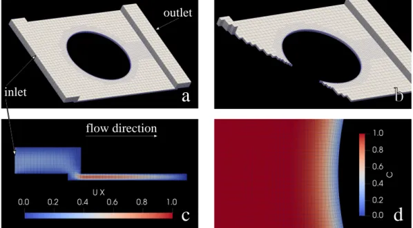
Simulations of reactive transport in fractured and porous media using the OpenFOAM toolkit have already been developed (Starchenko and Ladd, 2018; Starchenko et al., 2016). The pore-scale equations derived inAppendix Awere discretized on a finite-volume mesh. The mesh was constructed to represent the microfluidic device used in the experiments, including the reservoir regions that inject and extract fluid from above the channel. Illustrations of the model are shown inFig. 2. The top-left panel (2a) shows the whole device, with the blue lines indicating the decomposition of the fluid volume into individual cells. The three images2(a–c) have a fourfold coarser mesh than was used in the simulations; otherwise the mesh lines would be too closely spaced to be visible. The soluble surface of the gypsum chip is represented by an initially cylindrical surface, which is merged with the mesh of the microfluidic cell using the OpenFOAM utility snappyHexMesh. The region around the disk includes two forms of refinement. It is first re-fined with respect to the background mesh and then six to eight layers of cells are inserted so that the mesh matches as smoothly as possible to
the surface of the gypsum. A cutaway view (2b) gives additional in-formation as to how the mesh is resolved in the vicinity of the disk.
Fluid enters and leaves the channel from above, as illustrated in Fig. 2c, and quickly develops the typical parabolic profile. The ex-perimental device injects (and extracts) fluid through a bank of 8 in-jector pipes (seeFig. 1), whereas in the simulations fluid is injected and extracted uniformly across the extremities of the device (inlet and outlet). In either case the flow becomes uniform as soon as it enters the channel; the entrance length, 0.1Re h, is only 0.017 mm. The mean velocity in the channel, u0= 0.016835 mm s−1, is matched to the
volumetric flow rate in the experiment Q = 1 ml/hr.
Charge neutrality couples the motion of ions with different mobi-lities, and over distances larger than the Debye length both species diffuse at the same speed. For simplicity, we therefore consider a single species with a limiting diffusion coefficient D0= 9 × 10⁻⁴mm2s−1,
which is an average of the individual ion diffusivities (Alt-Epping et al., 2014). The simulations make use of the large time-scale separation between dissolution and transport (approximately 250-fold) to solve the coupled equations for flow, transport and dissolution sequentially. The mesh can be assumed to be fixed while the steady-state flow and transport equations (Appendix A) are solved.Fig. 2d shows the con-centration field at the leading edge of the disk at the resolution of the simulations. The strikingly smooth variation of the concentration field is a result of the mesh conforming precisely to the mineral-fluid inter-face.
Gypsum dissolution kinetics have been observed to follow a linear rate law R = k(csat− c) over most of the saturation range, with a rate
constant for polycrystalline samples k ≈ 4 − 5 × 10⁻³ mm s−1
(Colombani, 2008). In this paper we use k to represent the surface rate constant (in m s−1) and κ to represent the geochemical rate constant (in
M m−2s−1). The two rate constants are connected by the saturation
concentration of gypsum κ = kcsat, with csat = 15.2 M m−3
(Christoffersen and Christoffersen, 1976). There are orders of magni-tude variation in the rate constants reported in the literature (Colombani, 2008), as indicated inTable 1, but applying corrections for the thickness of the diffusive boundary layer and for the reactive sur-face area of granular samples, gives a reasonably consistent value for the dissolution rate constant, κ = 7 × 10⁻⁵ M m−2 s−1, which
translates to k = 4.5 × 10⁻³mm s−1. We use this value for k in most of
the numerical simulations.
Within a time-independent framework for flow and transport, there is only a single time scale, td= l0/kγ, which is the time it takes for the
mineral surface to retreat a distance l0when in constant contact with
pure water (we take l0= 1 mm). The parameter γ is the relative molar
volumes of the (porous) mineral and aqueous calcium phases, Eq. (A.13), and determines the interface velocity for a given reaction rate. A time unit in the simulation (with k = 4.5 × 10⁻³mm s−1) corresponds
to a real time td= 27.5 h for the sculpting plaster samples (50%
por-osity) and td= 21.4 h in the case of the analytical grade gypsum (61%
porosity). There are no fitting parameters involved in calculating the time scales.
We have carried out simulations with three different mesh resolu-tions, doubling the number of mesh points per direction at each stage. After 600 h of dissolution, there were small but noticeable differences in the size and shape of the gypsum chip at the coarse and intermediate resolutions, but no difference between the intermediate and fine re-solutions. We use the intermediate resolution in the rest of this study (illustrated inFig. 2d). After a time corresponding to about 600 h of real time, the mesh becomes distorted and the accuracy starts to decline. However, it is straightforward to create a new mesh whenever neces-sary by first writing the mineral surface coordinates to a stereo-lithography (STL) file and then using this triangulated surface mesh as input to a new volume mesh. In this way we can track the evolving shape down to a few percent of the original volume. Since the fields are stationary in time, they are completely specified by the location of the surface points. Once a new mesh has been created the simulation can be
restarted without any interpolation of the fields. However, external remeshing adds a computational overhead, so it is done as infrequently as possible. We have verified that the results are insensitive to the frequency of remeshing.
3. Results
Results from this study examine the underlying assumptions of pore-scale modeling with a new level of detail and precision. Despite the simplicity of the system (gypsum and water), it was not straightforward to match the predictions of the simulations with the experimental ob-servations. The reaction rate constant is sensitive to small impurities in the sample so that dissolution rates measured from samples created by rehydrating plaster of Paris are significantly less than for samples made from analytical grade gypsum hemihydrate. From the modeling per-spective, numerical simulations suggest that the effects of concentration on the ion diffusion coefficients are needed to account for the observed dissolution rates.
3.1. Dissolution of plaster of Paris
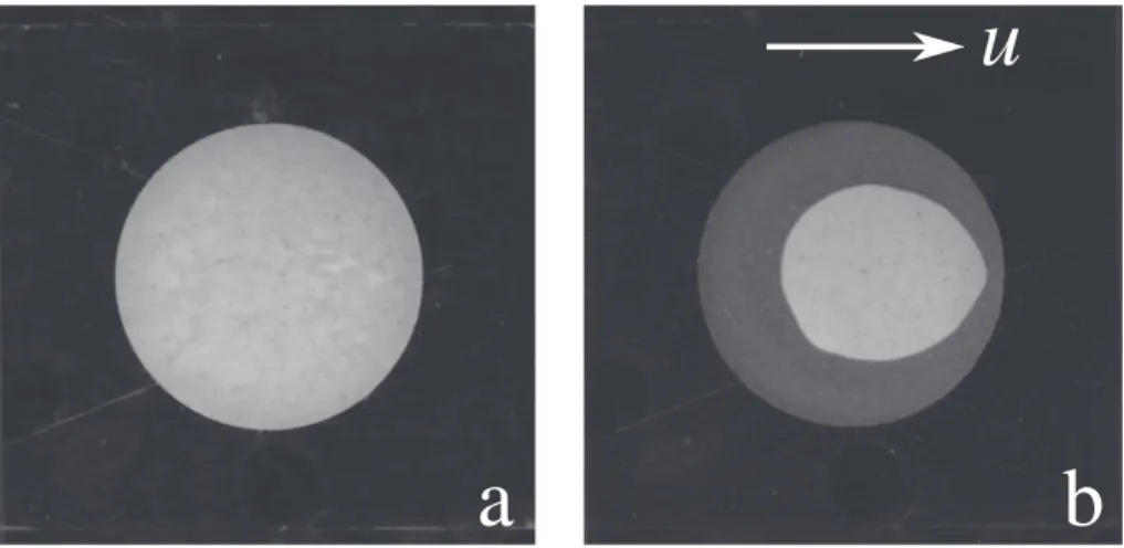
Images of a sample of rehydrated plaster of Paris and the same sample after 900 h of dissolution are shown inFig. 3. The disk remains more or less symmetric top to bottom, but there is a fore-aft asymmetry, with the trailing edge developing a sharp cusp over time (Section 3.6). The outline of the initial (circular) shape is caused by insoluble mate-rials that are added to the powdered CaSO4hemihydrate, and which
settle to the bottom of the cell once the gypsum dissolves. Videos of these experiments are in the Supplementary Material (pA1.mp4 and pA2.mp4).
The decrease in sample volume reflects the local dissolution flux integrated over the exposed surface Dn c dS. The sample is confined by the polycarbonate plates (Fig. 1) and no fluid flows across the top and bottom surfaces. The exposed surface area is the perimeter of the disk, initially 2πa, multiplied by its height h = 0.5 mm.Fig. 4shows the volume of the dissolving chip as a function of time for two different experiments, along with numerical simulations (circles) using the methodology described inSection 2.2. Time dependent volumes mea-sured in the two experiments are almost identical (red and blue lines), but clearly different from numerical simulations (red circles) using the expected surface reaction rate k = 4.5 × 10⁻³mm s−1(Colombani,
2008). The simulated sample dissolves about twice as fast as the ex-perimental samples, which cannot be plausibly explained by un-certainties in k. Due to the large diffusional hindrance, a reaction rate approximately five times smaller k = 0.9 × 10⁻³mm s−1(blue circles)
is needed to approach the observed dissolution rate (dV/dt). This dis-crepancy requires further investigation, which will be discussed in Section 3.3.
The inset toFig. 4shows that the simulation and experimental data initially agree rather well, but after approximately 40 h of dissolution, the rate (measured by the slope of the time-dependent volume of the chip) decreases significantly. We suggest that the initial slope reflects the actual dissolution rate of gypsum; subsequently the dissolving sur-face becomes passivated by a layer of additives which slows the dis-solution (as intended by the manufacturer).
a
d
c
b
inlet
outlet
flow direction
Fig. 2. Simulation of the microfluidic cell: a) the microfluidic device with the gypsum cylinder as empty space. Fluid fills the meshed region only. The surface of the
cylindrical hole moves inwards as the solid dissolves. b) A cutaway of the system illustrating the mesh refinements in the region of the disk. c) A cross section of the inlet region (y = W/2 = 16.5 mm) showing the flow into the channel. d) A portion of the mesh near the stagnation point illustrating the different levels of mesh refinement used in the simulations; the color field indicates the dimensionless undersaturation (A.11).
Table 1
Selected results for the rate constant of gypsum dissolving in water. The mea-surement methods include a spinning disk (disk), batch dissolution (batch), digital holographic microscopy (DHM), a channel-flow cell (CFC), and the mi-crofluidic experiment reported here (micro). The experiments used either single crystals or polycrystalline samples. We used solubility data fromChristoffersen and Christoffersen (1976)to obtain the dissolution rate constants fromBarton and Wilde (1971)andMbogoro et al. (2011). The geochemical rate constants (κ) can be converted to reaction rate constants (k) by dividing by csat= 15.2 M
m−3(Christoffersen and Christoffersen, 1976).
Reference κ(×105M m−2s−1) Method Sample
Barton and Wilde (1971) 100 Disk Poly
Raines and Dewers (1997) 350 Disk Poly
Jeschke et al. (2001) 11 Disk Poly
Palandri and Kharaka (2004) 160
Colombani and Bert (2007) 5 DHM Single
Colombani (2008) 7 Poly
Mbogoro et al. (2011) 9 CFC Single
Lebedev (2015) 15 Batch Poly This work 7–14 Micro Poly
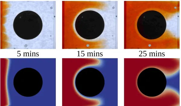
3.2. Advection-diffusion of a passive tracer in the microfluidic device To eliminate a potential source of the discrepancy in dissolution rates (Section 3.1), an experiment was made to validate the simulation of reactant transport in the microfluidic device. A saturated CaSO4
so-lution, colored with a marker dye, was injected into the inlet, and the transport of a non-reactive tracer into the cell was observed by frequent imaging (4 frames per second). This could be compared with a simu-lation of the same process, as a check of the flow and transport com-ponents of the simulation. Illustrative results are shown inFig. 5, which track the infiltration of a tracer concentration over a time period of 25 min.
It can be seen that the simulations capture the main features of the experimental observations, including the halo around the disk formed by a boundary layer approximately 1 mm thick. This is not the typical concentration boundary layer because there is no flux at the cylinder surface. Instead, it is a transient effect caused by the slow diffusion of reactant across the stream lines and the absence of convection towards the disk surface. Eventually the halo disappears and the concentration in the whole cell becomes uniform. The time for the reactant
concentration to reach its (uniform) steady state is approximately 1 h, much less than the dissolution time td> 20 h.
In the first frame of the experiment, sinusoidal variations in the front position are visible. These are clearly correlated with the positions of the injectors, and in future experiments we will investigate if these variations can be suppressed by adding a diffuser plate to the flow stream. Nevertheless the front becomes smooth before it encounters the disk and we do not think this has a significant effect on the transport of ions from the disk.
3.3. Effects of impurities on the reaction rate constant
InFig. 3we saw evidence of insoluble impurities in the layer of dust left behind by the dissolving gypsum. Additives in sculpting plaster have chemical functions which include inhibiting dissolution of the hardened plaster. InFig. 6we compare the time-dependent volumes from a typical plaster experiment (dashed red line) with two more re-cent experiments using analytical grade (99.6% pure) CaSO4 (solid
lines). Visual observations (videospB1.mp4andpB2.mp4) confirm that the amount of insoluble material left behind has been significantly re-duced, although not entirely eliminated.
Surprisingly, the results inFig. 6show that the long-time dissolution rate of pure gypsum (solid lines) is about twice as fast as sculpting plaster (dashed red line) and in much better agreement with simulation (blue circles). A factor of two in the overall dissolution rate (dV/dt) reflects about a fivefold change in the reaction rate constant, because of the relatively slow transport of ions across the concentration boundary layer.
Although the agreement between simulation and experiment is significantly closer with analytical grade gypsum samples, as opposed to ones prepared from sculpting plaster, the simulations still predict a faster dissolution than is found experimentally, by about 20%. Rate constants for single crystals are about 30% smaller, but not enough to account for the differences shown in Fig. 6. Moreover the gypsum samples prepared in this work have a large porosity (61%) and might be expected to have a higher dissolution rate than more consolidated samples. This suggests we should look for other sources of hindrance to dissolution, specifically the reduction of ion diffusion coefficients by the high concentration boundary layer around the disk, which has an ionic strength up to 40 mM.
3.4. Activity corrections to ion diffusion
In the concentration boundary layer around the disk, the ionic strength is approximately 40 mM, even after taking account of the ion complexation reaction (2). This leads to an additional hindrance to ion
Fig. 3. Dissolution of sculpting plaster in a Hele-Shaw cell. A cylindrical sample is dissolved by the flow of water around its perimeter; the flow is from left to right. a)
Initial sample b) After 38 days of dissolution; the original shape of the chip can be inferred from the visible layer of insoluble material on the base of the cell.
Fig. 4. Sample volume V, normalized by its initial value V0, is plotted as a
function of time for two experiments (solid lines); the samples were made from sculpting plaster (pAx). Results from numerical simulations with reaction rates
k = 4.5 × 10⁻³mm s−1(red circles) and k = 0.9 × 10⁻³mm s−1(blue
circles) are shown for comparison. The inset figure shows short time dissolution from experiment (pA2S) and simulation (k45S) on an expanded scale. The added S in the legend names indicates the same experiment or simulation, but with more frequent sampling.
diffusion, caused by the interaction between neighboring ion clouds (Onsager and Fuoss, 1931);
= + D c D d d c ( ) 1 ln ln , 0 (3) where γ is the ion activity coefficient and c is the calcium ion con-centration.
The activity coefficients can be connected to the total calcium concentration using extended Debye-Hückel theory,
= +
± AB CC
ln 1
1 1 , (4)
where C is the normalized undersaturation, C = 1 − c/csat. The ionic
strength of saturated CaSO4(40 mM) is well within the limits of the
theory (I < 0.1 M). The coefficients A and B are related to parameters in the extended Debye-Hückel theory. The coefficient A = 1.151 was determined from the low-density limit of the activity coefficient, while B = 0.55 was determined by fitting data at higher concentrations to results from PHREEQC (Parkhurst and Appelo, 2013). The fit is essen-tially perfect over the whole saturation range and automatically in-cludes the reduction in ionic strength due to complexation (2).
Simulations have been carried out with and without activity cor-rections to the diffusivity. The undersaturation (C) and diffusivity (D) fields around the initial gypsum cylinder are shown inFig. 7. Since the flow is convection dominated (Pe = u0a/D0= 185) there is a thin
Fig. 5. Advection-diffusion of a passive tracer: an experiment using colored ink as a marker (top), and simulated concentration fields (bottom) at 5, 15, and 25 min.
The yellow contour line in the simulation results is drawn at 50% saturation.
Fig. 6. Effect of sample impurities on the dissolution rate. Results from
ex-periments using sculpting plaster (pA2, dashed red line) are compared with experiments using samples made from analytical grade hemihydrate (pBx, solid lines). The numerical simulation (k = 4.5 × 10⁻³mm s−1) is shown by solid
circles.
Fig. 7. Undersaturation (C) and diffusion (Deff) fields around a cylindrical disk. The color scale indicates the variation in concentration (left) and effective diffusion
concentration boundary layer, approximately 1 mm thick, around the leading edge of the cylinder. The fore-aft asymmetry develops because the solution is largely saturated before it reaches the trailing edge of the disk. The variation in concentration results in a varying diffusivity, with a broad minimum in the high-concentration (low C) region at the trailing edge of the cylinder. We can expect that the concentration-dependence of the diffusivity will impact the evolving shapes of the dissolving cylinder.
The activity correction to the diffusion coefficient increases the dissolution timescale by about 20%, bringing the simulations into near perfect agreement with experiment, as shown inFig. 8. The solid lines are results of experiments (fromFig. 6) and the circles are simulations with (red) and without (blue) activity corrections to D. It should be emphasized that there are no undetermined parameters in these com-parisons; the surface reaction rate is the literature value, k = 4.5 × 10⁻³mm s−1(Colombani, 2008). The inset figure shows
that including the activity correction extends the agreement between simulations and experiments made with sculptor's plaster (pA2) to over 80 h, compared with 40 h for the uncorrected diffusivity (Fig. 4). This shows that dissolution over short timescales (<80 h) is unaffected by the presence of the retardants and additives in commercial plaster. 3.5. Sensitivity of dissolution rate to the surface reaction rate
To investigate the sensitivity of dissolution rate to the reaction rate constant we have made additional simulations with k = 9 × 10⁻³mm
s−1, again including the activity correction to the diffusion coefficient.
InFig. 9the volume evolution from the two rate constants (blue and green circles) is compared with experiments pB1 (black line) and pB2 (blue line). Because dissolution in this system is largely controlled by the transport of ions across the concentration boundary layer, the overall dissolution rate is only weakly dependent on the reaction rate constant. The smaller reaction rate, k = 4.5 × 10⁻³mm s−1 (blue
circles), gives better agreement with the experiments, but the differ-ences are smaller than the effects of activity correction and comparable with the uncertainty in the experimental measurements.
One further experiment (red line) was made in which the flow rate was increased by a factor of four half-way through the experiment, after 353 h of dissolution. Movies illustrating the evolution of the sample (video pBX4.mp4) and the corresponding simulation (k45AX4.mp4) can be found in the Supplementary Material. Even before the increase in flow rate, the volume from experiment pBX4 is slightly but fairly
consistently below the volumes from pB1 and pB2 (150 h < t < 350 h). The reason for the more rapid dissolution in this experiment is not clear, but may be related to a higher ambient temperature. A simulation with the larger rate constant (k = 9 × 10⁻³mm s−1) matches the
volume change with time almost exactly up to 450 h, although the differences between the two rate constants are again small (see inset to Fig. 9.)
3.6. Time evolution of shapes
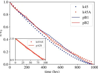
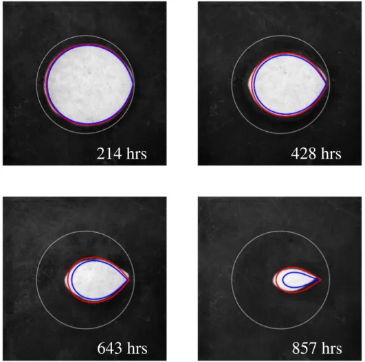
Results fromSections 3.4and3.5focus on global dissolution rates, averaged over the whole reactive surface of the sample. We can probe how local reaction rates vary in space and time by examining the evolving shape of the chip.Fig. 10shows images from experiment pB2 with simulated shapes at the corresponding time (within a one hour window) superposed on the photograph. The simulation with activity corrections to the diffusion coefficient (red lines) is in excellent agreement with experiment; on the other hand, the simulation with uncorrected diffusivity (blue lines) dissolves too quickly.
The sample shown inFig. 10(pB2) takes on a somewhat asymmetric shape after about 300 h of dissolution; in other experiments (Fig. 11) it remains symmetric. Nevertheless, towards the end of the experiment its shape again becomes very regular (Fig. 10). This suggests that, unlike many dissolution processes (Kondratiuk et al., 2017; Ortoleva et al., 1987; Szymczak and Ladd, 2014), a single grain dissolves stably. We have also noticed that the shapes of disks placed in different positions in the simulation cell (along the flow direction) could be superposed, again suggesting that shape formation is a stable process.
Fig. 11shows the observed and simulated shapes for experiment pBX4, where the flow rate was quadrupled after approximately 350 h of dissolution. The larger Péclet number reduces the time scale for com-plete dissolution from 1000 h to 700 h. The simulation is in near perfect agreement with experiment for the first 500 h, but dissolves more slowly towards the end of the experiment. The excellent agreement between simulated shapes and experimental observations for experi-ments pB1 and pB2, as well as the first half of pBX4, is confirmation of the underlying soundness of the model. The more rapid dissolution towards the end of pBX4 may reflect changes in experimental condi-tions that have not been accounted for, such as fluctuacondi-tions in ambient temperature or variations in sample porosity.
Fig. 8. Simulations of gypsum dissolution with constant diffusivity (blue
cir-cles) and with activity-corrected diffusivity (red circir-cles). Results from two ex-periments under similar conditions (pB1 and pB2) are shown by the solid lines. The simulations used the same reaction rate k = 4.5 × 10⁻³mm s−1. The inset
figure compares short time dissolution of plaster (pA2S) with a simulation in-cluding activity correction (k45AS).
Fig. 9. Simulations of gypsum dissolution with different reaction rate constants:
k = 4.5 × 10⁻³mm s−1(blue and black circles) and k = 9 × 10⁻³mm s−1
(green and red circles). Experimental results (pB1, pB2 and pBX4) are shown by the solid lines. The inset figure shows simulations of the pbX4 experiment (red line) with the same two rate constants: k = 4.5 × 10⁻³mm s−1(black circles)
4. Discussion
Mineral dissolution rates are frequently expressed in forms derived from transition-state theory (Lasaga, 1981, 1984). Experimental mea-surements (Colombani, 2008; Colombani and Bert, 2007; Mbogoro et al., 2011; Pachon-Rodriguez and Colombani, 2013) support a linear rate law for gypsum dissolution,
= M S c c 1 , R sat (5)
whereM is the rate of production of calcium ions (M s−1), S
Ris the
reactive surface area (m2), and κ is the dissolution rate constant per unit
area of reactive surface (M m−2 s−1). However, there are two key
sources of uncertainty in such experiments: the magnitude of the re-active surface area and the appropriate value of the concentration (Colombani, 2008).
The reactive surface area of crushed samples, as determined from a BET isotherm, is generally larger than the geometric area (Colombani, 2008; Jeschke et al., 2001), but in rock cores it can be smaller (Noiriel et al., 2009), making estimates of the rate constant less certain. How-ever, in microfluidic experiments the reactive area can be precisely determined as a function of time from the perimeter of the grain (e.g. Fig. 10), eliminating one source of uncertainty. A spinning disk (Barton and Wilde, 1971; Jeschke et al., 2001) or channel-flow (Mbogoro et al., 2011) geometry also allows for precise measurement of the reactive area, but individual grains generate more complex flows, which evolve in time as the mineral dissolves. The competition between surface and diffusional hindrance changes as the grain dissolves (dissolution
becomes more reaction limited), making for a more stringent test of the underlying physical model of the dissolution processes.
In analyzing batch experiments it is frequently assumed that the concentration appearing in the rate equation (5) is the same as the bulk concentration cB, but this is only true when the reaction rate is
suffi-ciently small that diffusional hindrance can be neglected. In general, the reactive flux R (M m−2s−1) is a local quantity that varies over the
surface of the dissolving mineral grain, =
R c( )S k c(sat cS) (6)
where cSis the (Ca2+) concentration at a specific point on the mineral
surface. The left panel ofFig. 7 shows that the concentration field around a single grain is not at all homogeneous. Instead the channel is mostly filled with pure fluid (c = 0 or C = 1), with a thin boundary layer around the disk where all of the concentration variation occurs. The difference between cSand cBis due to diffusional hindrance.
The effect of diffusional hindrance on the dissolution rate can be estimated by introducing the boundary layer thickness δ, replacing the diffusive flux in Eq. (A.8), D(n·∇c), by an effective flux D(cS− cB)/δ,
where cBis the concentration outside the boundary layer. The surface
concentration is then determined by a balance between the diffusion of ions away from the mineral surface and the rate of ion production by dissolution,
= D
c c k c c
(S B) (sat S). (7)
Solving for cSwe can rewrite Eq. (5) in terms of an effective rate
con-stant,
Fig. 10. Shapes of a dissolving gypsum chip; images from experiment pB2. The red lines indicate the simulated shapes, including activity corrections (k45A), at the
=
M k S ceff R(sat cB), (8)
where keffcontains an estimate of the diffusional hindrance
= +
k k D
1 1
.
eff (9)
In channel-flow cells or spinning-disk experiments, δ is constant and can be calculated analytically (Gregory and Riddiford, 1956; Szymczak and Ladd, 2012). However,Fig. 7shows that for more complex surfaces the thickness of the boundary layer varies over the mineral surface and Eq. (9) is only an approximation.
Mineral dissolution in the microfluidic setup is only weakly de-pendent on reaction rate constant; a factor of five reduction in k only decreases the dissolution time scale by a factor of two. Doubling the rate constant (k = 9 × 10⁻³mm s−1) leads to a marginally worse fit to
the experiments pB1 and pB2 (Fig. 9). On the other hand, the dissolu-tion of experiment pBX4 is better accounted for by the higher reacdissolu-tion rate, although again the difference is fairly small (inset toFig. 9). The more rapid dissolution in pBX4 may be caused by an increase in am-bient temperature over the duration of the experiment (4 weeks). Un-fortunately, it is not feasible at present to maintain a tight temperature control while simultaneously photographing the dissolving chip. Nevertheless, the uncertainty in reaction rate is small in comparison to the variation in published results (seeTable 1).
The presence of additives in commercial plasters has a surprisingly large effect on the dissolution rate constant. Sculpting plaster (pAx) and analytical grade gypsum samples (pBx) dissolve with similar reaction rates in the initial stages (inset toFig. 8). However, the rate constant of sculpting plaster decreases about fivefold after 100 h of dissolution. We
assume that this is due to additives in commercial plasters that are designed to reduce dissolution and better preserve the finished product. A high purity gypsum is needed for quantitative comparisons with si-mulations (Fig. 6). Activity corrections to the ion diffusion coefficient reduce the predicted dissolution rate, bringing the results into better agreement with experiment (Fig. 8), particularly in light of the higher reaction rate constant that might be expected for these highly porous (61%) samples.
Inspection of the V(t) plot for experiment pBX4 (Fig. 9) indicates an abrupt increase in slope after 420 h, unrelated to the change in flow rate that occurred at 350 h; at this point the experiment and simulation start to deviate. In general, the magnitude of dV/dt decreases with time because of the reduced surface area; in this case dV/dt increases by approximately 10%. One possible explanation is that the porosity of the sample is not entirely homogeneous. A 2% increase in porosity (from 61% to 63%) changes the dissolution time scale (tdin Eq. (A.13)) by
5%, which brings the simulated and experimental areas into sig-nificantly better agreement. If the central portion of the disk had a slightly larger porosity than the perimeter, this might account for the change in time scale in the latter half of the experiment. A much larger increase in reaction rate would be needed to accomplish the same ef-fect, because of the diffusional hindrance.
5. Conclusions
Microfluidic experiments, particularly when combined with nu-merical simulations, can complement traditional batch measurements of dissolution rates by elucidating the complex coupling between
Fig. 11. Shapes of a dissolving gypsum chip; images from experiment pBX4 (varying flow rate). The red line is the simulated shape with activity corrections
transport and surface chemistry over the wide range of scales that are typical in porous media. By using imaging instead of concentration measurements we can determine both local dissolution rates, from changes in shape (Figs. 10and11), and global dissolution rates from changes in sample volume (Figs. 4, 6,8, and9). However, in order to determine reaction rate constants from these measurements we must take account of diffusional hindrance across the boundary layer around the sample. Numerical simulations are needed in this case because of the complex flow lines around the grain.
In this paper we have confirmed that dissolution rates can be cal-culated from first principles, without any fitting parameters. The fun-damental equations for reactive transport were able to predict local dissolution rates, reflected in the changes in shape of an initially cy-lindrical sample, as well as global dissolution rates, as measured by the change in volume of the sample. There were no fitting parameters in these simulations, unlike previous studies (Molins et al., 2020; Soulaine et al., 2017) where the reaction rate constant was treated as a free parameter and the ion diffusion coefficient of the water-ethanol solu-tion could only be estimated. Here the diffusion coefficients were taken from infinite dilution measurements and corrected for concentration using Onsager's limiting law (Onsager and Fuoss, 1931).
Despite the chemical simplicity of gypsum dissolution, the level of agreement shown in Sections 3.4 and 3.6 was not easily obtained. Plaster samples (pAx) dissolved at about half the rate of samples made from analytical grade hemihydrate (pBx) as shown inFig. 6. Moreover, sculptor's plaster showed two distinct dissolution time scales, as in-dicated by the change in slope around 75 h (dashed line inFig. 4); on the other hand the analytical grade sample dissolves on a single time scale. The presence of small amounts of impurity in the sculptor's plaster had a surprisingly large effect on the dissolution rate constant (a 5-fold reduction), but a smaller effect on the measured dissolution rate because of diffusional hindrance. It should be noted that the impurities in sculpting plaster are engineered for specific applications, and similar levels of naturally occurring impurities would be expected to have a less dramatic effect. Nevertheless, formation of passivation layers by in-soluble impurities might introduce significant uncertainty in estimated dissolution rates if not recognized in the analysis.
Noticeable discrepancies in the observed dissolution rate were still visible, even when analytical grade CaSO4was used. However, the high
solubility of gypsum (15 mM) suggested the possibility of hindered diffusion from ion-ion interactions; the leading-order corrections are proportional to c, and much larger than for neutral molecules. We found that corrections based on Debye-Hückel theory reduced the rate of diffusion through the concentration boundary layer by about 25% (Fig. 7), bringing about an excellent agreement with experiment (Fig. 8). The reaction rate constant used for these comparisons (7 × 10⁻⁵M m−2s−1) was taken from a meta-analysis of a number of
studies on polycrystalline samples (Colombani, 2008). The rate con-stant for low-index gypsum crystals is about 30% smaller (Colombani
and Bert, 2007), but the polycrystalline value seems more appropriate for our samples, which were rehydrated from the powdered hemi-hydrate.
The geometry used in the microfluidic experiments caused sig-nificant diffusional hindrance to dissolution. The large pore size (~ 10 mm) meant that the concentration boundary layer is fairly thick (~ 1 mm), even at high Péclet numbers, and the surface reaction con-tributes less than 20% of the total hindrance to dissolution. The value from Colombani (2008)fits two out of the three experiments (pBx) extremely well, better than a twofold higher rate constant (Fig. 9). The variance in published rate constants (seeTable 1) is much larger than the uncertainties in this work (which are roughly a factor of two). Our results are consistent with the meta-analysis inColombani (2008)and also with more recent measurements on single crystals (Colombani and Bert, 2007; Mbogoro et al., 2011). More accurate rate constants could be obtained with variants of this experiment aimed at reducing the thickness of the boundary layer. Nevertheless, the key purpose of this work – a local validation of the pore-scale methodology – was accom-plished.
Supplementary data to this article can be found online athttps:// doi.org/10.1016/j.chemgeo.2019.119459.
Declaration of competing interest
The authors declare that they have no known competing financial interests or personal relationships that could have appeared to influ-ence the work reported in this paper.
Acknowledgments
We gratefully acknowledge the advice and support from Prof. Piotr Garstecki (Polish Academy of Sciences) in setting up the microfluidic experiments, and for comments on the manuscript. We thank the ASTAT Company (Poznań, Poland) for providing us with the ultrathin double-coated tape used in the experiments). Numerical data was generated with the OpenFOAMⓇ toolkit (v1712), http://www.
openfoam.com/. Source codes and sample input files used to produce the numerical data shown in this paper can be found athttps://github. com/vitst/dissolFoam/releases/tag/v1712. Additional output data is available on request. AJCL was funded by the U.S. Department of Energy, Office of Science, Office of Basic Energy Sciences, Chemical Sciences, Geosciences, and Biosciences Division under Award Number DE-SC0018676. Research by VS was sponsored by the Laboratory Directed Research and Development Program of Oak Ridge National Laboratory, managed by UT-Battelle, LLC, for the U. S. Department of Energy. FD, FO, SM and PS acknowledge the support by the National Science Center (Poland) under research grant no. 2012/07/E/ST3/ 01734.
Appendix A. Equations for pore-scale reactive transport
We consider a fluid volume confined by the microfluidic cell illustrated inFig. 2. The channel region is 33 mm wide, 0.5 mm high and is bounded by vertical planes at x = 0 and x = 38 mm. Fluid enters and exits the channel from above through an area 1 mm × 33 mm. The reservoir regions are filled and drained through the inlet (x = −4 mm) and outlet faces (x = 38 mm). Fluid is excluded from the region representing the gypsum chip by an initially cylindrical surface.
Fluid flow under the conditions of the experiment can be described by the stationary Navier-Stokes equations
+ =
uu p u
( ) 2 , (A.1)
where ν is the viscosity of the fluid and the pressure p is determined by the incompressibility condition, =
u 0. (A.2)
The Reynolds number in the experiments (based on the initial diameter of the sample) is 0.33, so inertial terms are small. Transport of reactants follows a convection-diffusion equation
+ u =
c ( )c (D c),
where c is the concentration field and D is the molecular diffusion coefficient. Since dissolution of a solid matrix is extremely slow in comparison with the time scales for reactant transport (Starchenko et al., 2016; Szymczak and Ladd, 2012), the stationary limit of the convection-diffusion equation,
=
uc D c
( ) ( ), (A.4)
can be invoked, except for the infiltration experiment shown inFig. 5.
Eqs. (A.1)–(A.4) are closed by zero-flux conditions on the surfaces of the microfluidic cell:
= = =
n p 0, u 0, n c 0, (A.5)
where the surface normal n points out of the fluid domain. At the inlet a uniform fluid velocity and concentration are imposed across the face:
= = =
n p 0, u u n c
4 , 0;
0
(A.6) the mean velocity in the channel, u0= 0.016835 mm s−1, is matched to the volumetric flow rate in the experiment Q = 1 ml/h. The factor of 1/4
accounts for the larger cross-sectional areas of the inlet in comparison to the channel. The outlet conditions are:
= u= n n =
p 0, u c
4 , 0.
0
(A.7) On the mineral surface the diffusive flux of ions from the surface must match the dissolution flux due to chemical reactions R:
= = =
n p 0, u 0, D(n c) R c( ), (A.8)
where R is the rate of production of ions at the mineral surface. Experimental studies of gypsum dissolution typically use a linear rate law to fit the data (Colombani, 2008; Colombani and Bert, 2007; Jeschke and Dreybrodt, 2002; Jeschke et al., 2001),
=
R c( )S k c(sat cS) (A.9)
where R is the surface reaction rate (M m−2s−1), c
Sis the concentration of calcium ions at the mineral surface and csatis the saturation
con-centration. We will use the same linear rate law (A.9), and assume that both cations and anions have the same (average) diffusion coefficient
= ++
D (DCa2 DSO24)/2so that only a single species needs to be tracked. Beyond the Debye screening length the solution is electrically neutral; thus the faster diffusing species (Ca2+) will drag the more slowly diffusing counterions (SO
4 2 ). The local dissolution flux controls the (normal) motion of points on the mineral surface,
= = r n n n v t R D c 1 d d ( ) , m (A.10)
where vm≪c−1is the molar volume of the consolidated mineral (74 cm3) and ϕ is the porosity of the gypsum grain.
The numerical simulations use the dimensionless undersaturation =
C c c
c ,
sat
sat (A.11)
instead of concentration. The boundary condition on the dissolving surface S is then
+ =
n
D( C) kC 0, (A.12)
and the motion of the boundary points can be calculated from the evolution equation =
r n n
t D C
d
d ( ) . (A.13)
The parameter γ = csatvm/(1 − ϕ) is the relative molar volume of the (porous) mineral and aqueous calcium phases; for the sculpting plaster samples
(pAx, ϕ = 0.50) γ = 0.00225, while for the pure gypsum samples (pBx, ϕ = 0.61) γ = 0.00288. In the paper we define a dissolution time scale, td= l0/kγ, to convert from the time units of the simulation to hours. We take l0= 1 mm as a characteristic length scale, so that tdreflects the time it
takes the mineral interface to retreat a distance of 1 mm (l0) while in constant contact with pure water (no transport hindrance).
The dissolution velocity from Eq. (A.13) is use to move the surface mesh points for some fraction of the dissolution time, typically 0.1td. After this,
the mesh points are relaxed by Laplacian smoothing to preserve mesh quality. The implementation of the mesh motion is discussed in detail in Starchenko and Ladd (2018).
References
Alt-Epping, P., Tournassat, C., Rasouli, P., Steefel, C.I., Mayer, K.U., Jenni, A., Mäder, U., Sengor, S.S., Fernández, R., 2014. Benchmark reactive transport simulations of a column experiment in compacted bentonite with multispecies diffusion and explicit treatment of electrostatic effects. Comput. Geosci. 19, 535–550.https://doi.org/10. 1007/s10596-014-9451-x.
Barton, A., Wilde, N., 1971. Dissolution rates of polycrystalline samples of gypsum and orthorhombic forms of calcium sulphate by a rotating disc method. Trans. Faraday Soc. 67, 3590–3597.https://doi.org/10.1039/tf9716703590.
Chen, L., Kang, Q., Tang, Q., Robinson, B.A., g He, Y.L., Tao, W.Q., 2015. Pore-scale simulation of multicomponent multiphase reactive transport w ith dissolution and precipitation. Int. J. Heat Mass Transf. 85, 935–949.https://doi.org/10.1016/j. ijheatmasstransfer.2015.02.035.
Christoffersen, J., Christoffersen, M.R., 1976. The kinetics of dissolution of calcium sul-phate dihydrate in water. J. Cryst. Growth 35, 79–88. https://doi.org/10.1016/0022-0248(76)90247-5.
Colombani, J., 2008. Measurement of the pure dissolution rate constant of a mineral in
water. Geochim. Cosmochim. Acta 72, 5634–5640.https://doi.org/10.1016/j.gca. 2008.09.007.
Colombani, J., Bert, J., 2007. Holographic interferometry study of the dissolution and diffusion of gypsum in water. Geochim. Cosmochim. Acta 71, 1913–1920.https:// doi.org/10.1016/j.gca.2007.01.012.
Colón, C.F.J., Oelkers, E.H., Schott, J., 2004. Experimental investigation of the effect of dissolution on sandstone permeability, porosity, and reactive surface area. Geochim. Cosmochim. Acta 68, 805–817.https://doi.org/10.1016/j.gca.2003.06.002. De Baere, B., Molins, S., Mayer, K.U., François, R., 2016. Determination of mineral
dis-solution regimes using flow-through time-resolved analysis (FT-TRA) and numerical simulation. Chem. Geol. 430, 1–12.https://doi.org/10.1016/j.chemgeo.2016.03. 014.
Gregory, D.P., Riddiford, A.C., 1956. Transport to the surface of a rotating disc. J. Chem. Soc. N/A, 3756–3764.https://doi.org/10.1039/JR9560003756.
Hodson, M.E., 2006. Does reactive surface area depend on grain size? Results from ph 3, 25 c far-from-equilibrium flow-through dissolution experiments on anorthite and biotite. Geochim. Cosmochim. Acta 70, 1655–1667.https://doi.org/10.1016/j.gca. 2006.01.001.
surface morphology. Geochim. Cosmochim. Acta 66, 3055–3062.https://doi.org/10. 1016/s0016-7037(02)00893-1.
Jeschke, A.A., Vosbeck, K., Dreybrodt, W., 2001. Surface controlled dissolution rates of gypsum in aqueous solutions exhibit nonlinear dissolution kinetics. Geochim. Cosmochim. Acta 65, 27–34.https://doi.org/10.1016/s0016-7037(00)00510-x. Kang, Q., Tsimpanogiannis, I.N., Zhang, D., Lichtner, P.C., 2005. Numerical modeling of
pore-scale phenomena during CO2 sequestration in oceanic sediments. Fuel Process. Technol. 86, 1351–1370.https://doi.org/10.1016/j.fuproc.2005.02.001. Kondratiuk, P., Tredak, H., Upadhyay, V., Ladd, A.J.C., Szymczak, P., 2017. Instabilities
and finger formation in replacement fronts driven by an oversaturated solution. J. Geophys. Res. Solid Earth 122, 5972—–5991.https://doi.org/10.1002/ 2017jb014169.
Landrot, G., Ajo-Franklin, J.B., Yang, L., Cabrini, S., Steefel, C.I., 2012. Measurement of accessible reactive surface area in a sandstone, with application to CO2 mineraliza-tion. Chem. Geol. 318-319, 113–125.https://doi.org/10.1016/j.chemgeo.2012.05. 010.
Lasaga, A.C., 1981. Transition state theory. In: Lasaga, A.C., Kirkpatrick, J. (Eds.), Kinetics of Geochemical Processes. vol. 8. De Gruyter, pp. 135–169.https://doi.org/ 10.1515/9781501508233.
Lasaga, A.C., 1984. Chemical kinetics of water-rock interactions. J. Geophys. Res. Solid 89, 4009–4025.https://doi.org/10.1029/jb089ib06p04009.
Lebedev, A.L., 2015. Kinetics of gypsum dissolution in water. Geochem. Int. 53, 811–824.
https://doi.org/10.1134/s0016702915070058.
Lichtner, P.C., Kang, Q., 2007. Upscaling pore-scale reactive transport equations using a multiscale continuum formulation. Water Resour. Res. 43, W12S15.https://doi.org/ 10.1029/2006WR005664.
Mbogoro, M.M., Snowden, M.E., Edwards, M.A., Peruffo, M., Unwin, P.R., 2011. Intrinsic kinetics of gypsum and calcium sulfate anhydrite dissolution: surface selective studies under hydrodynamic control and the effect of additives. J. Phys. Chem. C 115, 10147–10154.https://doi.org/10.1021/jp201718b.
Molins, S., Soulaine, C., Prasianakis, N.I., Abbasi, A., Poncet, P., Ladd, A.J., Vitalii Starchenko, S.R., Trebotich, D., Tchelepi, H.A., Steefel, C.I., 2020. Simulation of mineral dissolution at the pore scale with evolving solid-fluid interfaces: review of approaches and benchmark problem set. Comput. Geosci.https://doi.org/10.1016/ 0096-3003(89)90010-6.
Molins, S., Trebotich, D., Steefel, C.I., Shen, C., 2012. An investigation of the effect of pore scale flow on average geochemical reaction rates using direct numerical simulation. Water Resour. Res. 48.https://doi.org/10.1029/2011wr011404.
Molins, S., Trebotich, D., Yang, L., Ajo-Franklin, J.B., Ligocki, T.J., Shen, C., Steefel, C.I., 2014. Pore-scale controls on calcite dissolution rates from flow-through laboratory and numerical experiments. Environ. Sci. Technol. 48, 7453–7460.https://doi.org/ 10.1021/es5013438.
Noiriel, C., Luquot, L., Madé, B., Raimbault, L., Gouze, P., van der Lee, J., 2009. Changes in reactive surface area during limestone dissolution: an experimental and modelling study. Chem. Geol. 265, 160–170.https://doi.org/10.1016/j.chemgeo.2009.01.032. Oliveira, T.D., Blunt, M.J., Bijeljic, B., 2019. Modelling of multispecies reactive transport on pore-space images. Adv. Water Resour. 127, 192–208.https://doi.org/10.1016/j. advwatres.2019.03.012.
Onsager, L., Fuoss, R.M., 1931. Irreversible processes in electrolytes. Diffusion, con-ductance and viscous flow in arbitrary mixtures of strong electrolytes. J. Phys. Chem. 36, 2689–2778.https://doi.org/10.1021/j150341a001.
Ortoleva, P., Chadam, J., Merino, E., Sen, A., 1987. Geochemical self-organization II: the reactive-infiltration instability. Am. J. Sci. 287, 1008–1040.https://doi.org/10.
2475/ajs.287.10.1008.
Osselin, F., Budek, A., Cybulski, O., Kondratiuk, P., Garstecki, P., Szymczak, P., 2016. Microfluidic observation of the onset of reactive infiltration instability in an analog fracture. Geophys. Res. Lett. 43, 6907–6915.https://doi.org/10.1002/
2016gl069261.
Pachon-Rodriguez, E.A., Colombani, J., 2013. Pure dissolution kinetics of anhydrite and gypsum in inhibiting aqueous salt solutions. AIChE J. 59, 1622–1626.https://doi. org/10.1002/aic.13922.
Palandri, J.L., Kharaka, Y.K., 2004. A compilation of rate parameters of water-mineral interaction kinetics for application to geochemical modeling. In: Technical Report. US Geological Survey, Menlo Park, California.http://pubs.usgs.gov/of/2004/1068/. Parkhurst, D.L., Appelo, C.A.J., 2013. Description of input and examples for PHREEQC
version 3–A computer program for speciation, batch- reaction, one-dimensional transport, and inverse geochemical calculations. In: Technical Report. U.S. Geological Survey. http://pubs.usgs.gov/tm/06/a43.
Pereira Nunes, J.P., Blunt, M.J., Bijeljic, B., 2016. Pore-scale simulation of carbonate dissolution in micro-ct images. J. Geophys. Res. Solid Earth 121, 558–576.https:// doi.org/10.1002/2015JB012117.
Raines, M.A., Dewers, T.A., 1997. Mixed transport/reaction control of gypsum dissolution kinetics in aqueous solutions and initiation of gypsum karst. Chem. Geol. 140, 29–48.
https://doi.org/10.1016/s0009-2541(97)00018-1.
Rimstidt, J.D., Brantley, S.L., Olsen, A.A., 2012. Systematic review of forsterite dissolu-tion rate data. Geochim. Cosmochim. Acta 99, 159–178.https://doi.org/10.1016/j. gca.2012.09.019.
Soulaine, C., Roman, S., Kovscek, A., Tchelepi, H.A., 2017. Mineral dissolution and wormholing from a pore-scale perspective. J. Fluid Mech. 827, 457–483.https://doi. org/10.1017/jfm.2017.499.
Starchenko, V., Ladd, A.J.C., 2018. The development of wormholes in laboratory scale fractures: perspectives from three-dimensional simulations. Water Resour. Res. 54, 7946–7959.https://doi.org/10.1029/2018wr022948.
Starchenko, V., Marra, C.J., Ladd, A.J.C., 2016. Three-dimensional simulations of fracture dissolution. J. Geophys. Res. Solid Earth 121, 6421–6444.https://doi.org/10.1002/ 2016JB013321.
Steefel, C.I., Appelo, C.A.J., Arora, B., Jacques, D., Kalbacher, T., Kolditz, O., Lagneau, V., Lichtner, P.C., Mayer, K.U., Meeussen, J.C.L., Molins, S., Moulton, D., Shao, H., Šimůnek, J., Spycher, N., Yabusaki, S.B., Yeh, G.T., 2014. Reactive transport codes for subsurface environmental simulation. Comput. Geosci. 19, 445–478.https://doi.org/ 10.1007/s10596-014-9443-x.
Szymczak, P., Ladd, A.J.C., 2012. Reactive infiltration instabilities in rocks. Fracture dissolution. J. Fluid Mech. 702, 239–264.https://doi.org/10.1017/jfm.2012.174. Szymczak, P., Ladd, A.J.C., 2014. Reactive infiltration instabilities in rocks. Part 2.
Dissolution of a porous matrix. J. Fluid Mech. 738, 591–630.https://doi.org/10. 1017/jfm.2013.586.
Trebotich, D., Adams, M.F., Molins, S., Steefel, C.I., Shen, C., 2014. High-resolution si-mulation of pore-scale reactive transport processes associated with carbon seques-tration. Comput. Sci. Eng. 16, 22–31.https://doi.org/10.1109/MCSE.2014.77. Upadhyay, V.K., Szymczak, P., Ladd, A.J.C., 2015. Initial conditions or emergence: what
determines dissolution patterns in rough fractures? J. Geophys. Res. Solid Earth 120, 6102–6121.https://doi.org/10.1002/2015JB012233.
Vu, M.T., Adler, P.M., 2014. Application of level-set method for deposition in three-di-mensional reconstructed porous media. Phys. Rev. E 89, 053301.https://doi.org/10. 1103/PhysRevE.89.053301.