Desalination systems for the treatment of hypersaline produced water from unconventional oil and gas processes

Desalination Systems for the Treatment of

Hypersaline Produced Water from Unconventional

Oil and Gas Processes

by

Gregory P. Thiel

S.M., Massachusetts Institute of Technology (2012)

B.S.E, Case Western Reserve University (2010)

Submitted to the Department of Mechanical Engineering

in partial fulfillment of the requirements for the degree of

Doctor of Philosophy

at the

MASSACHUSETTS INSTITUTE OF TECHNOLOGY

June 2015

@

Massachusetts Institute of Technology 2015.

Sig

Author ...

Dep

Certified by...

Sig

A ccepted by ...

All rights reserved.

nature redacted

artme/ f Mechanical Engineering

May 5, 2015

iature redacted

John H. Lienhard V

bdul Latif Jameel Professor

1)

Thesi,, Supervisor

Signature redacted

David E. Hardt

Chairman, Department Committee on Graduate Theses

y TE

JUN 2 4 2015

LIBRARIES

ARCHNES

77 Massachusetts Avenue Cambridge, MA 02139

MfTLibraries

DISCLAIMER NOTICE

Due to the condition of the original material, there are unavoidable flaws in this reproduction. We have made every effort possible to provide you with the best copy available.

Thank you.

Despite pagination irregularities, this is the most complete copy available.

Desalination Systems for the Treatment of Hypersaline

Produced Water from Unconventional Oil and Gas Processes

by

Gregory P. Thiel

Submitted to the Department of Mechanical Engineering on May 5, 2015, in partial fulfillment of the

requirements for the degree of Doctor of Philosophy

Abstract

A combination of advances in drilling technology and the depletion of domestic con-ventional reserves has led to a boom in the use of hydraulic fracturing to recover oil and gas in North America. Among the most significant challenges associated with hydraulic fracturing is water resource management, as large quantities of wa-ter are both consumed and produced by the process. The management of produced water, the stream of water associated with a producing well, is particularly challeng-ing as it can be hypersaline, with salinities as high as nine times seawater. Typical disposal strategies for produced water, such as deep well injection, can be unfeasi-ble in many unconventional resource settings as a result of regulatory, environmen-tal, and/or economic barriers. Consequently, on-site treatment and reuse-a part of which is desalination-has emerged as a strategy in many unconventional formations.

However, although desalination systems are well understood in oceanographic and brackish groundwater contexts, their performance and design at significantly higher salinities is less well explored.

In this thesis, this gap is addressed from the perspective of two major themes: energy consumption and scale formation, as these can be two of the most significant costs associated with operating high-salinity produced water desalination systems. Samples of produced water were obtained from three major formations, the Marcel-lus in Pennsylvania, the Permian in Texas, and the Maritimes in Nova Scotia, and abstracted to design-case samples for each location. A thermodynamic framework for analyzing high salinity desalination systems was developed, and traditional and emerging desalination technologies were modeled to assess the energetic performance of treating these high-salinity waters. A novel thermodynamic parameter, known as the equipartition factor, was developed and applied to several high-salinity desalina-tion systems to understand the limits of energy efficiency under reasonable economic constraints. For emerging systems, novel hybridizations were analyzed which show the potential for improved performance. A model for predicting scale formation was developed and used to benchmark current pretreatment practices. An improved pre-treatment process was proposed that has the potential to cut chemical costs,

signifi-cantly. Ultimately, the results of the thesis show that traditional seawater desalination rules of thumb do not apply: minimum and actual energy requirements of hypersaline desalination systems exceed their seawater counterparts by an order of magnitude, evaporative desalination systems are more efficient at high salinities than lower salin-ities, the scale-defined operating envelope can differ from formation to formation, and optimized, targeted pretreatment strategies have the potential to greatly reduce the cost of treatment. It is hoped that the results of this thesis will better inform future high-salinity desalination system development as well as current industrial practice. Thesis Supervisor: John H. Lienhard V

Kurzfassung

Eine Kombination von technischem Vorsprung und der Verringerung der konven-tionellen Erdgas Ressourcen in Nordamerika hat zur Erweiterung der hydraulischen Aufbrechmethode geffihrt. Eine der wesentlichsten Herausforderungen dieses Ver-fahrens ist das Wasser Ressourcen Management, da das Verfahren eine groge Menge Wasser ben6tigt. Besonders schwierig ist die Behandlung des Abwassers, das zusam-men mit dem 01- oder Erdgasstrom aus der Quelle flieEt. Dieses Produktionswasser, das mit Salzgehalten bis zu neun mal Meerwasser als hypersalzig gekennzeichnet ist, muss in den meisten Fdllen beseitigt oder aufbereitet werden. Des Weiteren sind konventionelle Beseitigungsmethoden wie z.B. Tiefbrunnenentsorgung wegen u.A. gesetzlichen, umweltlichen, und 6konomischen Hindernissen bei unkonventionellen Ressourcen nicht immer m6glich. Deshalb ist vor Ort Abwasseraufbereitung, in der Entsalzung eine wesentliche Rolle spielen kann, neulich attraktiver geworden. Obwohl konventionelle Meerwasser Entsalzungsverfahren gut bekannt sind, sind die Leistungs-fahigkeiten und das Design dieser Systeme bei h6heren Salzgehalten in der 6ffentlichen Literatur nicht wohl erkundet.

Diese Dissertation konzentriert sich auf zwei Themen, die Thermodynamik und das Fouling dieser hypersalzigen Entsalzungssysteme, um zu versuchen, diese Licke teilweise zu ffillen. Ein thermodynamischer Rahmen fur die Bewertung und das Ver-standnis der konventionellen und neuen Entsalzungssystemen bei h6heren Salzge-halten wurde entwickelt und angewandt. Ein neues thermodynamisches MaE, der Equipartition Faktor, wurde entwickelt und verwendet, um das energetische Poten-zial der hypersalzigen Entsalzungssysteme unter realistischen wirtschaftlichen Bedin-gungen zu berechnen. Das Scaling, d.h., das Auskristallisieren von verschiedenen schwerl6slichen Salzen, wurde berechnet und vorausgesagt, um den Unterschied zwis-chen den ben6tigen Vorbehandlungsanforderungen in Meerwasser und Produktion-swasser Kontexten zu verstehen. Die Ergebnisse dieser Analyse wurden dann fur die Verbesserung des aktuellen Vorbehandlungsverfahrens verwendet. Schlieglich zeigen die Ergebnisse dieser Dissertationsarbeit, dass die Faustregeln fur das Verstdndnis der Meerwasserentsalzungssysteme nicht bei h6heren Salzgehalten gelten: der min-imale und tatsichliche Energieverbrauch kdnnen eine GrdIenordnung h6her als bei ozeanographischen Salzgehalten sein; Entsalzung durch Verdunstung ist effizienter bei h6heren Salzgehalten als bei niedrigeren; der Scaling-definierte Systembetriebsrah-men kann zwischen SchiefervorkomSystembetriebsrah-men sehr unterschiedlich sein; und zielorientierte, optimierte Vorbehandlungsverfahren k6nnen die Kosten der Produktionswasserauf-bereitung erheblich verringern. Es wird gehofft, dass die Ergebnisse dieser Arbeit die Weiterentwicklung der hypersalzigen Entsalzungsverfahren und auch die aktuellen industriellen Methoden besser informieren werden.

Acknowledgments

I owe a great debt of gratitude to my advisor, Professor John Lienhard, who has been a superb teacher, a constant source of guidance, and a trusted mentor. My deepest

thanks too are extended to my committee members, Professors Allan Myerson, Eve-lyn Wang, and Syed Zubair, whose steady support and regular feedback have been invaluable.

To my labmates both current and former in the Lienhard Research Group, I am thankful for your feedback, your insights, and the many inspiring discussions we have had. It has been a pleasure and an honor to work with each of you over the past five years. To those with whom I've worked closely, including Adam, Emily, Karan, Leo, Prakash, and Ronan: I thank you for challenging me, teaching me, and learning with me. I have come to believe that one of the highest values of an MIT education is the opportunity to be exposed to such a high concentration of intellectually-rich, motivated people with a wide diversity of background and thought, and you all truly exemplify that for me.

I am deeply grateful for the generous support of my sponsors. In particular, I would like to thank the King Fahd University of Petroleum and Minerals for funding the research reported in this thesis through the Center for Clean Water and Clean Energy at MIT and KFUPM. I would also like to extend my sincerest gratitude to the MIT Energy Initiative and the Martin Family Foundation for their fellowship support in my early years here.

And last but certainly not least, to my family and to my close friends in Cam-bridge: you have been my lifeline. I love you all.

Contents

1 Introduction: Water and Unconventional Oil and Gas 21

1.1 The Growth of Unconventional Oil and Gas . . . . 21

1.2 An Overview of Hydraulic Fracturing . . . . 24

1.3 Water Management in Hydraulic Fracturing . . . . 25

1.4 Thesis Aims and Overview . . . . 27

2 The Composition of Hypersaline Produced Water 31 2.1 Produced Water Field Samples . . . . 31

2.2 Design-Case Produced Water Samples . . . . 33

2.3 Modeling Hypersaline Waters of Diverse Composition . . . . 35

3 Understanding Energy Consumption in Hypersaline Desalination Systems 39 3.1 Introduction . . . . 40

3.2 A Thermoeconomic Framework for Assessment of Produced Water De-salination System s . . . . 40

3.2.1 Economic Rationale for Reuse . . . . 40

3.2.2 Modeling Produced Water Properties . . . . 41

3.2.3 Least Work of Separation . . . . 44

3.2.4 Second Law Efficiency . . . . 45

3.3 System s Analyses . . . .. . . . 46

3.3.1 Mechanical Vapor Compression . . . . 47

3.3.3 Forward Osmosis . . . . 55

3.3.4 Humidification-Dehumidification . . . . 60

3.3.5 _{Membrane Distillation . . . . 66}

3.3.6 Hypothetical High Salinity Reverse Osmosis . . . . 70

3.3.7 System Comparison . . . . 75

3.4 Conclusions . . . . 78

4 Improving Efficiency through Thermodynamic Equipartition 81 4.1 Introduction . . . . 82

4.2 _{Design for Equipartition . . . .} 83

4.3 Application of the Equipartition Factor . . . . 87

4.3.1 _{Lumped-Capacitance Systems . . . .} 87

4.3.2 Equipartition in a Building Heating System . . . . 89

4.3.3 Equipartition in Water Treatment Systems . . . . 93

4.4 Conclusions . . . . 98

5 Designing High-Salinity Desalination Systems for Equipartition 101 5.1 Introduction . . . . 102

5.2 Heat and Mass Exchanger Models . . . . 103

5.2.1 Effectiveness-NTU for Saline Evaporators . . . . 103

5.2.2 Effectiveness-MTU for Membrane Mass Exchangers . . . . 107

5.3 Redesigning Existing Systems for Equipartition . . . . 108

5.3.1 Mechanical Vapor Compression . . . . 109

5.3.2 Hypothetical High-Salinity Reverse Osmosis . . . .111

5.4 _{Designing New Systems for Equipartition . . . .111}

5.4.1 Mechanical Vapor Compression . . . . 112

5.4.2 Hypothetical High-Salinity Reverse Osmosis . . . . 113

5.5 Conclusions . . . . 115 6 Improving Efficiency through Hybridization with Pressure Retarded

6.1 Introduction . . . . 118

6.2 Process Description . . . . 119

6.3 Process Analysis . . . . 120

6.3.1 Reversible Process Analysis . . . . 122

6.3.2 Irreversible Process Analysis . . . . 123

6.4 Effective Efficiency Gain . . . . 124

6.5 Conclusions . . . . 125

7 Understanding Composition Effects on Scale Formation 127 7.1 Introduction . . . . 128

7.2 Method of Sample Analysis . . . . 128

7.2.1 Quantifying Supersaturation . . . . 128

7.2.2 Calculating the Saturation Index . . . . 129

7.2.3 Validation . . . . 137

7.3 The Variation of SI with Recovery, Temperature, and pH . . . . 139

7.3.1 Effect of Recovery Ratio . . . . 140

7.3.2 Effect of Temperature . . . . 144

7.3.3 Effect of pH . . . . 145

7.3.4 Combined Effects . . . . 147

7.4 Impacts on System Design and Selection . . . . 149

7.4.1 The Scale-Defined Operating Envelope . . . . 149

7.4.2 Options for Mitigation . . . . 151

7.5 C onclusions . . . . 151

8 Reducing Pretreatment Costs with Targeted Precipitation 153 8.1 Introduction . . . . 154

8.2 Baseline Process . . . . 154

8.2.1 Process Overview . . . . 154

8.2.2 Chemical Cost . . . . 155

8.3 Improved Process .. . . .. . . . . 156

8.3.2 Process Overview . . . . 159

8.4 Experimental Validation . . . . 161

8.4.1 Lab Setup and Procedure . . . . 162

8.4.2 R esults . . . . 162

8.5 Conclusions . . . .. . . . 163

A Thermodynamic Properties 165 A.1 Pitzer Equations . . . . 165

A.2 Effective Boiling Point Elevation . . . . 167

A.3 Thermodynamic Data . . . . 168

A.4 Least Work Curve . . . . 173

B Derivation of the Saturation Index 175 C Seawater FO-RO Model 177 D RO in the Produced Water Sector 179 D.1 Overview of Challenges to High-Salinity RO . . . . 179

List of Figures

1-1 Annual U.S. natural gas withdrawals by source . . . .

1-2 Mass of CO2 per unit energy of various fuels . . . .

1-3 Schematic diagram of hydraulic fracturing . . . .

3-1 3-2 3-3 3-4 3-5 3-6 3-7 3-8 3-9 3-10 3-11 3-12

Boiling point elevation and osmotic pressure of produced water . . . . Least work of separation vs. recovery ratio . . . .

Schematic diagram of mechanical vapor compression . . . .

Energy consumption of mechanical vapor compression vs. salinity . .

Mechanical vapor compression efficiency vs. salinity . . . .

Schematic diagram of multi-effect distillation . . . .

Energy consumption of multi-effect distillation vs. salinity . . . .

Multi-effect distillation efficiency . . . .

Schematic diagram of forward osmosis . . . .

Energy consumption of forward osmosis . . . .

Forward osmosis efficiency vs. salinity . . . .

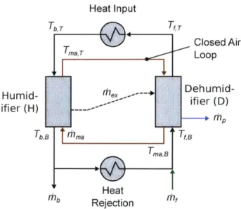
Schematic diagram of humidification-dehumidification . . . .

3-13 Enthalpy-temperature diagram of the humidification-dehumidification process... ...

3-14 Energy consumption of humidification-dehumidification vs. salinity 3-15 Schematic diagram of permeate gap membrane distillation . . . . 3-16 Differential control volume used in the PGMD model . . . . 3-17 Permeate gap membrane distillation energy consumption vs. salinity . 3-18 Schematic diagram of two-stage reverse osmosis . . . .

22 23 24 43 45 47 50 51 52 53 54 56 59 60 61 62 66 67 68 69 71

3-19 Energy consumption of hypothetical high-pressure reverse osmosis vs.

salinity . . . . 74

3-20 Efficiency of hypothetical high-pressure reverse osmosis vs. salinity . . 75

3-21 System efficiency comparison across the salinity domain . . . . 76

3-22 System efficiency comparison at produced water and seawater salinities 76 3-23 Energy consumption of systems at typical produced water salinities . 77 4-1 Efficiency of equipartitioned vs. non-equipartitioned systems . . . . . 86

4-2 Efficiency of equipartitioned, lumped-capacitance systems . . . . 89

4-3 Schematic diagram of a thermal storage heater . . . . 90

4-4 Temperature and entropy generation rates in the brick as a function of the dimensionless time, Fo = at/12 . . . . 92

4-5 Batch reverse osmosis processes . . . . 93

4-6 Hydraulic and osmotic pressures as a function of time . . . . 95

5-1 Differential control volume for effectivness-NTU analysis . . . 103

5-2 NaCl boiling point elevation curve with linearization . . . . 105

5-3 Effectiveness-NTU relationship for saline evaporators . . . 107

5-4 Equipartition factor and efficiency gains for MVC at fixed AT . . . . 110

5-5 Equipartition factor and efficiency gains for RO at fixed APt . . . 112

5-6 _{Equipartition factor and efficiency gains for MVC at fixed AT} . . . . 113

5-7 Efficiency of an equipartitioned MVC system . . . 114

5-8 Equipartition factor and efficiency gains for RO at fixed mean (A P-AH) 115 6-1 Schematic diagram of HDH and HDH-PRO hybrid . . . . 119

6-2 PRO mass flow rate ratio vs. HDH-PRO hybrid recovery ratio . . . . 121

6-3 Reversible work for a salinity gradient engine vs. salinity . . . . 122

6-4 Work output from a large PRO system vs. salinity . . . 124

6-5 Efficiency gain of HDH-PRO hybridization . . . 125

7-1 Calculation procedure for the saturation index, Eq. (7.2) . . . 130

7-3 7-4 7-5 7-6 7-7 7-8 7-9 7-10 7-11 7-12 7-13 7-14 7-15 7-16

Chemical softening process schematic drawing . . . . . Ettringite process schematic . . . . Conditions under which ettringite is supersaturated . . The potential for ettringite pretreatment . . . . Solid phases of calcium-aluminum-sulfate compounds

strength ... ...

Error estimation in solubility predictions . . . . Error estimation for sulfate SI calculations . . . .

Error estimation for NaCl SI calculations . . . . SI of chlorides vs. RR at T = 25'C and pH = 6 . . . . . SI of carbonates vs. RR at T = 25 0C and pH = 6 . . . . SI of sulfates vs. RR at T = 25'C and pH = 6 . . . .

SI of carbonates vs. temperature at RR = 0, and pH = 6 SI of sulfates vs. temperature at RR = 0, and pH = 6 . . SI of carbonate salts vs. pH at room temperature and RR SI of bases vs. pH at room temperature and RR = 0 . . . SI of NaCl vs. RR at elevated temperatures . . . . SI of carbonates vs. pH at high temperature and RR SI of bases vs. pH at high temperature and RR...

Scale-defined operating envelope . . . .

at high ionic

A-1 Least work of separation of NaCl solutions vs. feed salinity . . . . C-1 Schematic diagram of FO-RO for seawater desalination . . . .

-0 8-1 8-2 8-3 8-4 8-5 138 139 140 141 142 143 144 145 146 147 148 148 149 150 155 159 160 161 163 173 177

List of Tables

2.1 Composition of produced water field samples . . . . 2.2 Composition of design-case produced water samples . . . . .

4.1 Parameters for lumped-capacitance systems . . . .

4.2 Summary of the heat transfer system inputs and results . . . 4.3 Reverse osmosis base and redesign case results . . . .

8.1 Softening costs . . . .

8.2 Reagent data . . . . A. 1 The effective boiling point elevation (in K) for aqueous NaCl A.2 Standard state thermodynamic data for solid species . . . . A.3 Standard state thermodynamic data for aqueous species . . .

32 34 . . . . . 88 . . . . . 91 . . . . . 96 157 162 167 168 172

Nomenclature

Roman Symbols

A Area, m2

AO Modified Debye-Hiickel parameter, kg1/2_/moll/2

a Activity

Bij, Bfy Pitzer parameter, second virial coefficient, kg/mol

Bfy Pitzer binary interaction parameter, kg2_/mol 2

b Molality, mol/kg

C Electrical capacitance, F

Cij, CO Pitzer parameter, unlike-charged interactions, kg2_/mol2

c Concentration, mol/L; Specific heat capacity, J/kg K

Cp; c, Heat capacity at constant pressure, kJ/mol-K; kJ/kg-K

D Mass diffusivity, m2_/s

e Elementary charge, 1.602 176 565(35) x 10-19 C

F Extended Debye-Hiickel function; Faraday constant C/mol Fo Fourier number, at/l2

f

F'

G; g; a Gibbs free energy, J; J/kg; J/mol GOR Gained output ratio, fp hfg /Q

g; g' Pitzer function, Eqs. (A.7) and (A.8)

H; h Enthalpy, kJ/mol; kJ/kg

h Heat transfer coefficient, W/m2 _K

hm Mass transfer coefficient, m/s

hfg Enthalpy of vaporization, kJ/kg

I Ionic strength, mol/kg

i Current density, A/m2

j Flux

K Equilibrium constant

Ksp Solubility product

k Thermal conductivity, W/m K

kA Membrane permeability, kg/m2-h-bar

kB Boltzmann constant, J/K

L Generalized force-flux coefficient

1 Length, m

M Molar mass, kg/mol

MR Mass flow rate ratio

m Mass, kg

M" Mass flux, kg/m2_-s

Th Mass flow rate, kg/s

N Molar flow rate, mol/s

Q

Q

q Heat flux, W/m2

P Pressure, Pa

PR Pressure ratio

R Gas constant, J/mol-K or J/kg-K; Resistance, Q RR, RR Mass- and mole-based recovery ratio

S Supersaturation ratio

Strans Entropy transferred, J/K Sgen Entropy generation, J/K Sgen Entropy generation rate, W/K SI Saturation index, log(Q/K.9) SPR Single pass recovery ratio

T Temperature, 0C or K

TDS Total dissolved solids, mg/L or mg/kg

t Time, s

U Internal energy, J

V Volume, m3/mol or m3/kg; voltage, V vW Partial molar volume of water, m3/mol

W;W Work, J or kWh; W

w Mass fraction

Y Generalized system state

Z Pitzer function, E mi Izi, mol/kg

z Charge number

Roman Symbols

m Molality, mol/kg

Am Membrane permeability, kg/m2h bar

w Specific work, kWh/m3

y Salinity, kg/kg

Greek Symbols

a _{Pitzer parameter, kg21/mol"; Thermal diffusivity, m}2

_/s

#3w

#?

17 Molal activity coefficient; ratio of specific heats

7+Y Mean molal activity coefficient

Ar Change of reaction

Af Change of formation

6 Boiling point elevation, K

Cr Relative permittivity

EO Vacuum permittivity, F/m r7 Second law efficiency

0 Pitzer parameter, kg/mol; Dimensionless temperature difference

rX Characteristic inverse time, 1/s

Aj4 Pitzer parameter, uncharged interactions, kg/mol

A Chemical potential, J/mol

V Stoichiometric coefficient Equipartition factor Exergy flow rate Dummy variable

H Osmotic pressure, bar

p Density, kg/m3

pA Partial density of species i, kg/m3

0- Electrical conductivity S/m; Supersaturation (percent)

T Characteristic time, s

<Ij, <bf Pitzer parameter, like-charged interactions, kg/mol

VJ' 3 Pitzer parameter, like-charged interactions, kg2/mol2

'Jijk Pitzer parameter, ternary interactions, kg2

_/mol

<0 Osmotic coefficient; Electrical potential, V

w Humidity ratio, kgv/kgaa

Subscripts

0 Dead state; initial state

a, X Anion

B Bottom

b Brine stream; or brick

C Compressor c Capacitor c, M Cation D Dehumidifier d Draw stream da Dry air

dc Concentrated draw stream

dd Diluted draw stream

EC Evaporator-Condenser

e Equipartitioned

eff Effective

ex Extracted stream

f Feed stream

H High pressure; high temperature; humidifier

HP Heat pump i Inlet ib Intermediate brine im Intermediate value L Low ma Moist air

n, N Neutral species

ne Non-equipartitioned

o Outlet

P Pump

p Product (fresh or treated) stream

pp Pinch point PX Pressure exchanger RO Reverse Osmosis r Recirculated stream rec Recovered rev Reversible s Salt; source sat Saturated T Top; total t Terminal; turbine v Vapor

w, W Pure water; or wall

Superscripts

ex Excess thermodynamic quantity

s Saturated state

o Reference state

Chapter 1

Introduction: Water and

Unconventional Oil and

Gas

A combination of reduced conventional reserves, policy changes, and advances in drilling technology has paved the way for a natural gas boom in North America. Much of this new resource is recovered using an unconventional technique known as hydraulic fracturing, in which small fissures are created in a narrow, tight shale layer

to release bound up hydrocarbons. Much of the controversy surrounding this process has focused on its nexus with water, as significant quantities of water are associated

with each stage of a fractured well's life cycle. In particular, the challenges associated with source water competition and wastewater disposal are driving increased recy-cling and reuse, part of which is achieved by desalination. This chapter provides an

introduction to unconventional oil and gas, reviews some of the literature on water-related challenges, and concludes with the specific motivation for developing a deeper

understanding of desalination systems for hypersaline produced water.

1.1

The Growth of Unconventional Oil and Gas

Owing to advances in drilling technology and increasing global demand, the use of hydraulic fracturing to recover abundant supplies of oil and natural gas has become

30

u, 25

-o20 15 -5

u 15From Gas Wells

(D

"U 10 From Shale Wells

From Oil Wells

5

Cl)

- From Coalbed Wells

0

1940 1950 1960 1970 1980 1990 2000 2010

Figure 1-1: Annual U.S. natural gas withdrawals from 1940-2013: The spike in do-mestic natural gas production over the past decade has been driven almost entirely

by unconventional sources, most dominant among which is shale gas produced using

hydraulic fracturing. Data from [5].

includes tight oil and gas, shale oil and gas, and coalbed methane. In a conventional resource, oil and/or gas are trapped in a semi-porous, relatively high-permeability reservoir by an impermeable seal; drilling through this seal into the reservoir allows hydrocarbons to escape up the well. In contrast, unconventional resources are char-acterized by their relatively low permeability, such that additional stimulation-the fracturing process-is required to recover hydrocarbons from the formation.

Among unconventional resources, the shale resource alone is vast worldwide. Ac-cording to the U.S. Energy Information Administration (EIA) [3,4], nearly 207 trillion cubic meters (7,299 trillion cubic feet, or tcf) of natural gas and 55 billion cubic me-ters (345 billion barrels) of oil are technically recoverable globally. In energetic terms, this corresponds to roughly 7.7 zettajoules' of gas and 2.1 zettajoules of oil-a near sixty-year supply of gas and a decade-long supply of oil at current rates of global consumption.

And it is this larger shale gas resource that has boomed in the U.S. As shown in Fig. 1-1, between 2007 and 2013, gas withdrawals from shale wells increased nearly

11 ZJ = 1021 j

C: 0t_-0 4L--0 C,, 120 100 80 60 40 20 0 o e ef z~> 91

0

Figure 1-2: Natural gas is among the cleanest burning hydrocarbons, with nearly half the CO2 produced per unit, energy as coal. Data from [7]; energetic content of fuels

based on the higher heating value.

sixfold-from 2 tef in 2007 to almost 12 tef 2013 [5]. This growth has eclipsed the concurrent, 25%X, decline in withdrawls from conventional gas wells to add more than

5 tcf to total gross withdrawals. The year-over-year growth in withdrawals from 2010

to 2011 was the highest since at least 1940, the beginning of available data from the EIA.

Although it's not a renewable resource, natural gas provides significant environ-mental benefits over other widely available fossil fuels (Fig. 1-2). Natural gas power-plants produce half as much carbon dioxide as a typical coal powerplant, and harmful emissions of nitrous oxides and sulfur oxides are reduced by 66% and 99%, respec-tively [6]. Mercury emissions are effecrespec-tively eliminated. In home heating, the com-bustion of natural gas produces 27% less CO2 than heating oil. Greater use of natural

gas at the expense of coal in particular would have a significant impact on reducing worldwide greenhouse gas (GHG) emissions, as the two largest GHG emitters, the

U.S. and China, produce 39% and 69% of their electricity from coal, respectively.

23

4. Flowback and 5. Wastewater Produced Water Treatment and

1. Water 2. Chemical 3. Well (Wastewaters) Waste Disposal Acqu tion Mixnjectio

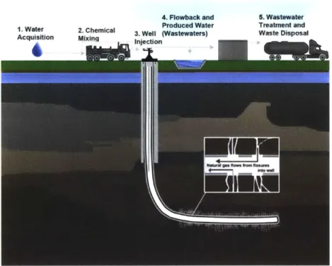
Figure 1-3: A schematic diagram of hydraulic fracturing: a high-pressure mixture of water, sand, and chemicals is pumped into a horizontal well in a deep, narrow shale layer to create small, microfissures and fracture the formation. The pressure at the top of the well is then released, allowing water and hydrocarbons to flow back up the well. (Image source: epa.gov)

1.2

An Overview of Hydraulic Fracturing

The technique with which oil and gas are recovered from shale layers is known as hydraulic fracturing (Fig. 1-3), and it works as follows. A vertical well is drilled to a depth of 1500-4500 in where it turns horizontally into a shale layer which may be as narrow as tens of meters in height [2]. A steel and cement casing is installed along the entire length of the bore. Then, a shaped-charge device known as a perforating gun creates holes in the casing and the surrounding shale layer. A high pressure mixture of sand, water, and chemical additives (about 84%, 15%, and 1% by mass, respectively) is pumped down the well to open up the starter holes created by the perforating gun and create microfissures, or to fracture, the shale [2,8]. The pressure at the top of the well is released, and a portion of the fracturing fluid flows back up the well. Much of the sand in the mixture remains behind to act as a "proppant," holding the microfissures open and allowing a continuous stream of hydrocarbons and

associated water to escape up the well.

1.3

Water Management in Hydraulic Fracturing

Among the most significant challenges associated with hydraulic fracturing is water resource management [9,10], as the process consumes and produces large amounts of water. Water consumption associated with hydraulic fracturing in the Barnett shale in Texas was equivalent to about 9% of Dallas water use in 2010 [11], and water use

for all oil and gas operations in Oklahoma is expected to reach 5% of state net use by 2060 [12].

Anywhere from 7,600-25,000 m3 _{(2-6.5 million gallons) [2, 13, 14] of water are}

used in the water-sand-chemical mixture [8] needed to perform a single fracture. Depending on the formation and well, between 15-70% of the fluid pumped down to

fracture the well will return to the surface as "flowback" at relatively high flow rates and relatively low total dissolved solids (TDS) [2]. After approximately one to three

weeks [13], the flow of water decreases significantly and the TDS increases sharply [15]. This subsequent stream is known as produced water, because it is associated with a producing well, and will continue to flow throughout the life of the well. The

low-salinity flowback can often be reused in subsequent fracturing operations with no or minimal treatment [16, 17]. In contrast, the produced water stream, which

at salinities as high as nine times seawater [2] can be hypersaline, must in general be treated or disposed of. Thus, despite the promise of hydraulic fracturing as a

technique to recover vast amounts of relatively clean-burning fuel, the management of hypersaline produced water is among the most significant barriers to expanded use of the process.

According to the U.S. Department of Energy, the total volume of produced water from all U.S. oil and gas production is 2.5 trillion cubic meters per year [18]. Account-ing for the portion of this attributable to unconventional gas production is difficult, but average federal, onshore water-to-gas ratios are estimated at about 1.46 L/m3 _[18],

60% of U.S. natural gas production in 2011, or about 388 billion cubic meters of gas. We might therefore estimate U.S. produced water generation from unconventional gas to be approximately 566 million cubic meters per year.

Conventional disposal procedures for these large quantities of produced water involve transporting the wastewater to a disposal well [17], where it is reinjected into the ground. Unfortunately, in the regions surrounding many unconventional formations, this process is fraught with difficulties arising from environmental and geological concerns, local regulatory frameworks, and high transportation costs. En-vironmentally, the disposal of wastewater via deep well injection has been linked to significantly increased seismicity [19], including cases in Arkansas [20], Ohio [21], and Oklahoma [22, 23]. In the Marcellus in Pennsylvania, a combination of regulatory issues and geological conditions make wastewater disposal via deep-well injection in-feasible. Operators in the Marcellus consequently transport the water across state

lines, to Ohio, where far more injection wells are available [24]. Economically, truck-ing costs are a strong function of the distance from the well to the disposal site and are significant-typically $25 per m3 _{($4 per bbl) in the Marcellus [25].}

On-site desalination is a part of the produced water. management solution that can address both environmental and economic challenges [26]. But in spite of a gen-eral trend towards reuse and work towards formalizing a water treatment selection process [27, 28], no overarching industry standard or regulatory requirement yet ex-ists on what treatment processes are necessary or best-suited for particular waters, or on the extent to which wastewater must be treated before reuse. Furthermore, solutions for desalinating hypersaline produced water streams in particular are un-standardized, with no clear and dominant choice among emerging and established technologies. And the selection of appropriate treatment technologies in the hyper-saline produced water context proves challenging as a result of: (1) the difficulty in characterizing hypersaline waters of extremely diverse composition; (2) the

desirabil-ity of high recovery ratios (i.e., highly concentrative treatment); and (3) significant variations in water composition from formation to formation and even well to well. Finally, though well-understood for seawater and brackish groundwater feeds, the

performance of desalination systems in treating hypersaline produced waters, is not well understood.

1.4

Thesis Aims and Overview

In this thesis, this gap in understanding the performance of-and how to improve-desalination systems that treat high salinity produced waters is addressed. More

broadly, the thesis seeks to answer the question, how do high salinities and diverse water compositions affect the performance of novel and established desalination tech-nologies? The question is answered in two parts, which correspond to two of the highest costs in treating produced water: the cost of desalination system energy con-sumption and the cost of pretreatment to prevent scale formation. In each part, the thesis seeks to understand the state of the art and suggest methods for improvements. A more detailed overview of the thesis follows.

Chapter 2

In Chapter 2, original samples of high salinity produced water from three major shale formations are presented: the Maritimes Basin in Nova Scotia; the Marcellus Shale in Pennsylvania; and the Permian Basin in Texas. The field samples are abstracted into three design-case samples, one for each formation. Finally, the Pitzer equations

are introduced to model the thermophysical properties of the samples.

Chapter 3

In this chapter, we provide models for calculating the energy consumption of produced water desalination technologies at high salinity and variable water composition in order to: (1) provide a baseline method for energetic comparison of produced water desalination technologies; (2) aid in the development of thermoeconomic models that

will better inform technology selection; and (3) provide a basis for further system research and development.

Chapter 4

In Chapter 4, a new dimensionless quantity, the equipartition factor, is defined. This

quantity, a function of the variance in dimensionless driving force throughout the sys-tem, is used to identify the improvement in efficiency achievable via system redesign

for a reduction in driving force variance, while holding fixed the system output for fixed system dimensions in time and space.

Chapter 5

In this chapter, we apply the equipartition design and rating strategy discussed

in Ch. 4 to understand the potential for improved energy efficiency in two

high-salinity desalination systems, reverse osmosis (RO) and mechanical vapor compression (MVC). For each system, we show (1) the best possible improvements in efficiency

from redesigning an existing system for equipartition; and (2) the best possible effi-ciency for a perfectly equipartitioned new system of a given physical size.

Chapter 6

In Chapter 6, a novel hybridization of brine-recirculating humidification-dehumidification (HDH) desalination with pressure retarded osmosis (PRO) is proposed and analyzed.

The proposed hybridization is shown to significantly increase efficiency of

low-single-pass-recovery desalination systems when treating typical, high-salinity produced wa-ter feeds to saturation.

Chapter

7

The aim of this chapter is to aid in the selection of produced water treatment tech-nology by identifying the temperature, pH, and recovery ratio under which mineral solid formation, or scale formation, is likely to occur. A maximum recovery ratio for

desalination systems treating water from each of the design-case samples is computed, and several likely problematic scales are identified.

Chapter 8

This chapter discusses an alternative pretreatement methodology to prevent the for-mation of the scales identified in Ch. 7. Results from modeling the improved process and a proof-of-concept experiment show the potential to reduce chemical dosing re-quirements significantly relative to current chemical softening techniques.

Chapter 2

The Composition of Hypersaline

Produced Water

In this chapter, samples of produced water from three formations are presented,

an-alyzed, and modeled. The field sample analysis reveals a diverse mix of ions and a broad range of total dissolved solids, both between and within the formations. The field samples are reduced to a single, representative design-case sample for each

for-mation. The thermophysical properties of these design-case samples are modeled using Pitzer's equations, which are applied in subsequent chapters to understand the behavior of these waters in desalination systems.

2.1

Produced Water Field Samples

We obtained three samples of produced water from the Permian Basin in Texas, USA; five samples from the Marcellus in Pennsylvania, USA; and four samples from the Maritimes Basin in Nova Scotia, Canada for assay. Water sample analyses were performed by Microbac Laboratories, Inc. of Worcester, Massachusetts. Each sample

was tested for 27 potential dissolved compounds: aluminum, arsenic, barium, beryl-lium, bicarbonate, boron, bromide, cadmium, calcium, chloride, chromium, cobalt, copper, iron, lead, lithium, magnesium, manganese, mercury, molybdenum, nickel, potassium, selenium, silver, sodium, strontium, and sulfate.

Table 2.1: Composition of water samples of produced water from unconventional oil and gas processes in the Permian Basin, Marcellus Shale, and the Maritimes Basin

Sample Concentration (mg/L)

Permian Marcellus Maritimes

Species No. 1 No. 2 No. 3 No. 1 No. 2 No. 3 No. 4 No. 5 No. 1 No. 2 No. 3 No. 4

Al3+ - - - - 0.26 -B - - - - - - - - 580 - 0.59 -Br- 1160 1650 1370 541 1820 872 1100 1678 - - - -Ba2+ 16 0 16 9700 9400 8900 2800 8923 - - 0.85 6 Ca2+ 14000 10000 15000 5400 23000 7600 13000 13875 - 920 670 773 Cl- 116000 111000 138000 66600 157000 91200 82800 115194 37900 63700 38300 33000 C02+, Co3 + - - - 8 8.2 6.8 - - - - - -Cu - - - - - - - - 0.072 -Fe2+, Fe3+ - - - 120 24 53 20 - - - -HCO- 108 92 160 48 - - - - 68 124 58 -K+ 840 570 1100 160 430 110 310 - - 200 83 37 Li+ - - - 130 170 85 90 369 - - - -Mg2+ 1650 1630 1950 492 1690 754 1380 1216 272 518 316 309 Mn2+ 42 11 53 6.9 9.3 - 5.1 4 - - 0.52 -Na+ 54000 48000 54000 33000 46000 33000 31000 46695 19000 32000 22000 19200 SO2- 743 530 515 1500 1040 550 - 26 - - - -Sr2+ 740 730 820 2700 7700 3300 3000 4064 20 8 7 8.7 TDS 189299 174213 212984 120406 248292 146431 135505 192044 57840 97470 61436 53334

The results are shown in Table 2.1. The total dissolved solids (TDS) varies widely, ranging from a low of about 53 g/L to a high of nearly 250 g/L, or roughly two to

seven times the TDS of seawater, and varies within each formation as well as between the formations. In addition, individual ion concentrations can vary significantly: in Permian Basin sample 2, the concentrations of Mn2+ and K+ differ by a factor

of about two and four, respectively, from the other two samples from the Permian Basin; boron is present at about 0.6 g/L in one sample but almost completely absent

in all of the others. Concentrations are not given where the result is lower than the resolution of the test. It should be noted that these samples do not perfectly (within

5-20%) satisfy electroneutrality, likely due to inaccuracies in chloride concentrations. Previous studies have also noted this discrepancy, and they adjusted the chloride

count as appropriate [13].

Unfortunately, data on dissolved silica, a common scale-forming compound, is unavailable from our samples. Other samples of Marcellus wastewater in open

liter-ature [13] show silica concentrations between 10 and 40 mg/L; in the Permian it is generally between 50 and 150 mg/L. With silica solubility between 100 and 150 mg/L

at room temperature [29], it may be problematic in the Permian, but appears less likely to be so in the Marcellus.

Any organic carbon may also have an impact on ion speciation and mineral solu-bilities, although this impact is considered negligible in seawater [30]. Total organic

carbon (TOC) data from our samples is unavailable, but TOC data from [13, 15] range from < 10 to 160 mg/L, and will at least in part depend on the method used for oil-water separation. Moreover, its effects on the solubilities of the compounds considered here would be difficult to quantify without knowing the makeup of the

TOC. We thus do not consider the effects further.

2.2

Design-Case Produced Water Samples

To capture the essential makeup of each region's produced water, a design-case sample

Table 2.2: Composition of design-case produced water samples Concentration

Permian Marcellus Maritimes

Species mg/L millimolal mg/L millimolal mg/L millimolal

Br- 1393 18.8 1202 15.4 Ba2+ 0.453 0.00356 0.268 0.002 1.6 0.0128 Ca2+ 13000 350 12575 322 568 15.1 Cl- 111000 3378 86457 2500 36221 1090 C02+ - - 6 0.104 CT 120 2.12 48 0.807 83 1.41 Fe2 + - - 54 1 K+ 837 23.1 253 6.63 77 2.1 Li+ - - 169 25 Mg2+ 1743 77.4 1106 46.7 340 14.9 Mn2+ 35 1.51 6 0.246 Na+ 53550 2513 37939 1692 22164 1030 SO- 596 6.69 779 8.32 Sr2+ 763 9.4 4153 48.6 11 0.128 TDS 183037 6379 144748 4667 59466 2154

to maintain electroneutrality and to ensure ambient conditions. The design-case data for

no compounds were supersaturated at the three regions are shown in Table 2.2. In each of the samples in Table 2.1, the maximum and minimum concentrations of individual ions generally vary by less than about 30-40% relative to their design case values in Table 2.2; however, some compounds (particularly iron, cobalt, sulfate, and strontium in the Marcellus) vary significantly more.

Several additional approximations were employed in the construction of the design-case from the field data:

" The water samples' pH are unavailable. Based on data from other hydraulic fracturing water literature (e.g., [13, 15, 31]), the pH is generally neutral to slightly acidic; we therefore assume a baseline pH of 6. (The pH is varied in model.)

* In the sample tests, dissolved inorganic carbon was reported as the concentra-tion of HCO3; in the design case it is quantified as total inorganic carbon, CT,

the sum of aqueous concentrations of C02, HCO-, H2CO3, and CO2-. The

value of CT is independent of pH.

" The sample tests do not distinguish between Fe2+ and Fe3+ or between C02+ and Co3_{+: absent data on dissolved oxygen concentrations, we cannot determine}

the relative proportions of either. We thus consider only the 2+ forms here.

* Concentrations in Table 2.2 are given in mg/L and millimolal. We have used densities of pure sodium chloride solutions in the conversion from mg/L to millimolal, i.e., mmol/kg solvent. For reference, a sodium chloride solution with a TDS of 60 ppt has a density of 1.040 kg/L at 25 C [32]; seawater has a density of 1.043 kg/L at the same TDS and temperature [33]. Of course, because the samples are fictitious and only intended to represent real water samples, an exact value is not needed for this conversion.

" Borates and dissolved copper are considered outliers and are not included in the design-case samples, as they were only present in significant amounts in one of the water samples shown in Table 2.1.

2.3

Modeling Hypersaline Waters of Diverse

Com-position

In order to predict the performance of desalination systems used to treat these waters, we require a model for the waters' thermodynamic properties. The Pitzer model has been widely applied to mixed electrolytes at high ionic strengths. It is based on a virial expansion of the Gibbs free energy, and accounts for ion interactions through pairwise and ternary parameters. Derivations can be found in, e.g., [34-36]. The

excess Gibbs free energy is given by

m eT= F +Z 1 _{bba[2Bca + Z~ca]}

C a

+ 1:( bebei 24cc, + 1 bax ccia

c<ci . a.

+ (( baba/ 2(Daal + 1: bc'Fcaaf (2.1)

a<ai .C. where 4A'kI F = -41.2 ln(1 + 1.2x/) (2.2) 1.2 A 1 e3 (2Npw) 1/2 (2.3) 3 [87r (crokBT) 31 2 Z = Zbizi (2.4)

and mw is the mass of pure water (solvent), R is the universal gas constant, b is molality, NA is Avogadro's number, e is the elementary charge, 6_{r is the relative} permittivity of pure water, EO is the vacuum permittivity, and kB is the Boltzmann constant. The subscripts c and a denote individual cation and anion species, respec-tively; sums over c < c' and a < a' denote sums over distinguishable pairs of cations and anions, respectively. The terms Bij, Cij, 4ij, and Tijk represent specific ion interactions between dissimilarly-charged pairs, like charged pairs, and ion triplets, respectively. The terms Bij and Qij are, in general, a function of ionic strength and the specific ion pair and are given in App. A. 1. Values of Cij and Tijk are tabulated. Equations for the dielectric constant as a function of temperature and pressure are given by Bradley and Pitzer [37], and data for the thermodynamic properties of wa-ter are taken from IAPWS [38]. Contributions to the excess Gibbs free energy from uncharged solutes can be represented by additional terms in Eq. (2.1) as required, as done in Ch. 7.

appropriately differentiated to obtain the thermodynamic properties of interest: the activity coefficients for predicting solid-liquid equilibrium (scale formation), and the osmotic coefficient, the heat capacity, and the excess volume for modeling system energy consumption. From standard thermodynamic relationships [39-41], the activ-ity coefficient of solute i, molal osmotic coefficient, specific heat capacactiv-ity, and excess volume are, respectively:

In -Yj (GexImwRT) (2.5) -1 abiGex(26 q5 - 1= RT~~(2.6) RT E_' bi amw C

(

)

In the chapters that follow, we use the Pitzer model in various forms to predict the potential for scale formation and methods for scale formation prevention, the energy consumption of high salinity desalination systems, and various ways to reduce energy consumption in these systems. The specific parameters and forms of the Pitzer equations used will depend on the application; the relevant details are described in the individual chapters as appropriate.

Chapter 3

Understanding Energy Consumption

in Hypersaline Desalination Systems

On-site treatment and reuse is an increasingly preferred option for produced water management in unconventional oil and gas extraction. This chapter analyzes and

compares the energetics of several desalination technologies at the high salinities and diverse compositions commonly encountered in produced water from shale formations

to guide technology selection and to inform further system development. Produced water properties are modeled using Pitzer's equations, and emphasis is placed on how these properties drive differences in system thermodynamics at salinities significantly

above the oceanic range. Models of mechanical vapor compression, multi-effect distil-lation, forward osmosis, humidification-dehumidification, membrane distildistil-lation, and a hypothetical high pressure reverse osmosis system show that for a fixed brine

salin-ity, evaporative system energetics tend to be less sensitive to changes in feed salinity.

Consequently, second law efficiencies of evaporative systems tend to be higher when treating typical produced waters to near-saturation than when treating seawater. In

addition, if realized for high-salinity produced waters, reverse osmosis has the poten-tial to achieve very high efficiencies. The results suggest a different energetic paradigm in comparing membrane and evaporative systems for high salinity wastewater

treat-The work in this chapter is based on [42] and benefited from the contributions of all coauthors. In particular, the sections on forward osmosis, reverse osmosis, and membrane distillation were led

ment than has been commonly accepted for lower salinity water.

3.1

Introduction

In this chapter, we provide models for calculating the energy consumption of produced water desalination technologies at high salinity and variable water composition in order to: (1) provide a baseline method for energetic comparison of produced water desalination technologies; (2) aid in the development of thermoeconomic models that will better inform technology selection; and (3) provide a basis for further system research and development.

3.2

A Thermoeconomic Framework for Assessment

of Produced Water Desalination Systems

In this section, we develop a simple thermoeconomic framework that informs the choice of thermodynamic figures of merit. We argue that when reuse is economically viable, recovery ratios should be maximized, and that energy consumption should be normalized per unit product water. We then discuss how composition affects energy consumption and the maximum recovery ratio attainable. Finally, we use these components to develop an approach to compare the energetics of desalination systems at produced water salinities.

3.2.1

Economic Rationale for Reuse

Where a regulatory framework does not compel a particular reuse or disposal process, economics will dictate the extent and type of reuse. The net water cost to a field operator is the sum of sourcing, reuse (if present), and disposal costs. In general, a reuse system splits a wastewater feed stream into a brine (or solids) and purer product

stream. Depending on the reuse strategy, the net cost of reuse may be reduced by the sale of valuable brine [43], blending, or partial desalination [44]. In spite of the

feed stream's disposal cost and the potential value of the brine and product streams, it is the product stream alone that reduces the quantities of both the water sourced and disposed. Thus, either high disposal or high sourcing costs can motivate reuse.

More precisely, the net cost of reuse per unit product must be less than the unit cost of sourcing and disposal for reuse to be economically justifiable. Consequently, the energy consumption, which is directly proportional to the net energetic cost, should

also be normalized per unit of product.

In addition, because produced water desalination is a waste concentration process, recovery ratios (the ratio of product to feed stream mass flow rates, RR = rp/7f)

should generally be maximized. Thus, for any desalination component of a reuse strategy, we require models describing energy consumption per unit water produced

and a method to determine the maximum recovery attainable, both of which depend on the produced water composition.

3.2.2

Modeling Produced Water Properties

Produced water composition and total salinity vary widely, not only from formation to formation, but even from well to well [13,45,46], making it impossible to standardize the composition. Nevertheless, the major components of the water show patterns.

In the samples presented in [45, 46], sodium and chloride make up the largest mass fraction of dissolved material, and about 95-98% of the solutes on a molal scale

are made up of calcium, sodium, and chloride ions. Other components are present in amounts less than 1%. Although these minor components will impact system design through, e.g., scaling considerations, they will not affect the separation energy

significantly. We thus propose that, for the purposes of thermodynamic analyses, the thermophysical properties of the water are mostly characterized by considering

mixtures of Ca-Na-Cl, in varying amounts. Because the addition of up to 10% calcium changes the properties only slightly (as shown below), we will only consider aqueous sodium chloride in the present work.

Thermophysical properties that affect the energy consumption of systems analyzed

osmotic pressure (H), all of which vary significantly over broad ranges of salinity. For an arbitrary mixture, these properties are computed according to:

1000 +

>i

P = -(3.1)

1000/pw + Zi biVo + Vex

-o

C, = AY+ bic~,. + Cex (3.2)

RT2_#bi

6= hf (3.3)

hfg

I = RTqpw bi (3.4)

where b is molality, M is molar mass, R is the universal gas constant,

#

To compute these properties, we require models for the excess volume, the excess heat capacity, and the osmotic coefficient that can be used for electrolytes at high ionic strengths. We use Pitzer's equations [34,35] for this purpose, which are outlined in Ch. 2 and have been validated for a wide array of single and mixed electrolytes over a range of concentrations from dilute to saturation [36,47]. We use values and correlations for the Pitzer parameters from [32] for NaCl; for CaCl2 they are taken

from [48]. Pure water properties are from the International Association for the Prop-erties of Water and Steam (IAPWS) [38] formulation.

The boiling point elevation and osmotic pressure of aqueous NaCl is shown in Fig. 3-1, with comparison to design-case samples from [46] for two major shale for-mations: the Permian Basin and the Marcellus. For the Permian sample, which is mostly NaCl, pure NaCl represents a good approximation to 6 and 1; in the Marcellus, where Ca2_{+ concentrations are higher, an Na-Ca-Cl mixture is a better}