Direct limits on the $B_s^0$ oscillation frequency

arXiv:hep-ex/0603029v2 17 Jul 2006

Direct Limits on the B

Oscillation Frequency

V.M. Abazov,36_{B. Abbott,}76 _{M. Abolins,}66_{B.S. Acharya,}29_{M. Adams,}52 _{T. Adams,}50 _{M. Agelou,}18 _{J.-L. Agram,}19

S.H. Ahn,31 _{M. Ahsan,}60 _{G.D. Alexeev,}36 _{G. Alkhazov,}40 _{A. Alton,}65_{G. Alverson,}64_{G.A. Alves,}2 _{M. Anastasoaie,}35

T. Andeen,54 S. Anderson,46 B. Andrieu,17 M.S. Anzelc,54 Y. Arnoud,14 M. Arov,53 A. Askew,50 B. ˚Asman,41 A.C.S. Assis Jesus,3 _{O. Atramentov,}58_{C. Autermann,}21 _{C. Avila,}8 _{C. Ay,}24 _{F. Badaud,}13 _{A. Baden,}62_{L. Bagby,}53

B. Baldin,51 _{D.V. Bandurin,}36_{P. Banerjee,}29_{S. Banerjee,}29_{E. Barberis,}64_{P. Bargassa,}81_{P. Baringer,}59_{C. Barnes,}44

J. Barreto,2_{J.F. Bartlett,}51_{U. Bassler,}17_{D. Bauer,}44_{A. Bean,}59 _{M. Begalli,}3 _{M. Begel,}72_{C. Belanger-Champagne,}5

A. Bellavance,68_{J.A. Benitez,}66 _{S.B. Beri,}27 _{G. Bernardi,}17 _{R. Bernhard,}42 _{L. Berntzon,}15 _{I. Bertram,}43

M. Besan¸con,18 _{R. Beuselinck,}44_{V.A. Bezzubov,}39 _{P.C. Bhat,}51 _{V. Bhatnagar,}27 _{M. Binder,}25 _{C. Biscarat,}43

K.M. Black,63_{I. Blackler,}44_{G. Blazey,}53_{F. Blekman,}44_{S. Blessing,}50_{D. Bloch,}19 _{K. Bloom,}68 _{U. Blumenschein,}23

A. Boehnlein,51 _{O. Boeriu,}56 _{T.A. Bolton,}60 _{F. Borcherding,}51_{G. Borissov,}43 _{K. Bos,}34 _{T. Bose,}78_{A. Brandt,}79

R. Brock,66_{G. Brooijmans,}71 _{A. Bross,}51_{D. Brown,}79 _{N.J. Buchanan,}50 _{D. Buchholz,}54 _{M. Buehler,}82

V. Buescher,23_{S. Burdin,}51_{S. Burke,}46 _{T.H. Burnett,}83 _{E. Busato,}17 _{C.P. Buszello,}44 _{J.M. Butler,}63 _{S. Calvet,}15

J. Cammin,72 _{S. Caron,}34_{W. Carvalho,}3_{B.C.K. Casey,}78_{N.M. Cason,}56 _{H. Castilla-Valdez,}33 _{S. Chakrabarti,}29

D. Chakraborty,53_{K.M. Chan,}72_{A. Chandra,}49_{D. Chapin,}78 _{F. Charles,}19_{E. Cheu,}46 _{F. Chevallier,}14 _{D.K. Cho,}63

S. Choi,32 _{B. Choudhary,}28 _{L. Christofek,}59 _{D. Claes,}68 _{B. Cl´ement,}19_{C. Cl´ement,}41 _{Y. Coadou,}5_{M. Cooke,}81

W.E. Cooper,51 _{D. Coppage,}59 _{M. Corcoran,}81_{M.-C. Cousinou,}15_{B. Cox,}45_{S. Cr´ep´e-Renaudin,}14 _{D. Cutts,}78

M. ´Cwiok,30H. da Motta,2 A. Das,63M. Das,61 B. Davies,43 G. Davies,44 G.A. Davis,54 K. De,79 P. de Jong,34 S.J. de Jong,35 _{E. De La Cruz-Burelo,}65_{C. De Oliveira Martins,}3 _{J.D. Degenhardt,}65_{F. D´eliot,}18 _{M. Demarteau,}51

R. Demina,72 _{P. Demine,}18 _{D. Denisov,}51 _{S.P. Denisov,}39 _{S. Desai,}73 _{H.T. Diehl,}51 _{M. Diesburg,}51 _{M. Doidge,}43

A. Dominguez,68 _{H. Dong,}73 _{L.V. Dudko,}38_{L. Duflot,}16 _{S.R. Dugad,}29 _{A. Duperrin,}15_{J. Dyer,}66 _{A. Dyshkant,}53

M. Eads,68_{D. Edmunds,}66_{T. Edwards,}45 _{J. Ellison,}49 _{J. Elmsheuser,}25_{V.D. Elvira,}51 _{S. Eno,}62 _{P. Ermolov,}38

J. Estrada,51 _{H. Evans,}55 _{A. Evdokimov,}37_{V.N. Evdokimov,}39_{S.N. Fatakia,}63 _{L. Feligioni,}63_{A.V. Ferapontov,}60

T. Ferbel,72 _{F. Fiedler,}25_{F. Filthaut,}35 _{W. Fisher,}51 _{H.E. Fisk,}51 _{I. Fleck,}23 _{M. Ford,}45 _{M. Fortner,}53 _{H. Fox,}23

S. Fu,51_{S. Fuess,}51_{T. Gadfort,}83 _{C.F. Galea,}35 _{E. Gallas,}51 _{E. Galyaev,}56 _{C. Garcia,}72 _{A. Garcia-Bellido,}83

J. Gardner,59_{V. Gavrilov,}37 _{A. Gay,}19 _{P. Gay,}13 _{D. Gel´e,}19_{R. Gelhaus,}49 _{C.E. Gerber,}52 _{Y. Gershtein,}50

D. Gillberg,5 _{G. Ginther,}72 _{N. Gollub,}41_{B. G´omez,}8 _{K. Gounder,}51 _{A. Goussiou,}56 _{P.D. Grannis,}73 _{H. Greenlee,}51

Z.D. Greenwood,61 _{E.M. Gregores,}4 _{G. Grenier,}20_{Ph. Gris,}13 _{J.-F. Grivaz,}16 _{S. Gr¨unendahl,}51 _{M.W. Gr¨unewald,}30

F. Guo,73 _{J. Guo,}73 _{G. Gutierrez,}51_{P. Gutierrez,}76 _{A. Haas,}71_{N.J. Hadley,}62_{P. Haefner,}25 _{S. Hagopian,}50

J. Haley,69 _{I. Hall,}76 _{R.E. Hall,}48 _{L. Han,}7 _{K. Hanagaki,}51_{K. Harder,}60 _{A. Harel,}72 _{R. Harrington,}64

J.M. Hauptman,58 _{R. Hauser,}66_{J. Hays,}54 _{T. Hebbeker,}21 _{D. Hedin,}53 _{J.G. Hegeman,}34 _{J.M. Heinmiller,}52

A.P. Heinson,49 U. Heintz,63 C. Hensel,59 G. Hesketh,64 M.D. Hildreth,56 R. Hirosky,82 J.D. Hobbs,73 B. Hoeneisen,12 _{M. Hohlfeld,}16 _{S.J. Hong,}31_{R. Hooper,}78 _{P. Houben,}34 _{Y. Hu,}73 _{V. Hynek,}9 _{I. Iashvili,}70

R. Illingworth,51 _{A.S. Ito,}51 _{S. Jabeen,}63 _{M. Jaffr´e,}16_{S. Jain,}76 _{V. Jain,}74 _{K. Jakobs,}23_{C. Jarvis,}62_{A. Jenkins,}44

R. Jesik,44_{K. Johns,}46 _{C. Johnson,}71 _{M. Johnson,}51 _{A. Jonckheere,}51 _{P. Jonsson,}44 _{A. Juste,}51 _{D. K¨afer,}21

S. Kahn,74_{E. Kajfasz,}15 _{A.M. Kalinin,}36_{J.M. Kalk,}61_{J.R. Kalk,}66_{S. Kappler,}21_{D. Karmanov,}38_{J. Kasper,}63

I. Katsanos,71D. Kau,50 R. Kaur,27R. Kehoe,80 S. Kermiche,15 S. Kesisoglou,78A. Khanov,77 A. Kharchilava,70 Y.M. Kharzheev,36 _{D. Khatidze,}71_{H. Kim,}79 _{T.J. Kim,}31_{M.H. Kirby,}35 _{B. Klima,}51 _{J.M. Kohli,}27_{J.-P. Konrath,}23

M. Kopal,76 _{V.M. Korablev,}39 _{J. Kotcher,}74 _{B. Kothari,}71_{A. Koubarovsky,}38_{A.V. Kozelov,}39 _{J. Kozminski,}66

A. Kryemadhi,82 _{S. Krzywdzinski,}51 _{T. Kuhl,}24 _{A. Kumar,}70 _{S. Kunori,}62_{A. Kupco,}11 _{T. Kurˇca,}20,∗_{J. Kvita,}9

S. Lager,41_{S. Lammers,}71 _{G. Landsberg,}78_{J. Lazoflores,}50_{A.-C. Le Bihan,}19 _{P. Lebrun,}20_{W.M. Lee,}53_{A. Leflat,}38

F. Lehner,42 _{C. Leonidopoulos,}71 _{V. Lesne,}13 _{J. Leveque,}46 _{P. Lewis,}44_{J. Li,}79 _{Q.Z. Li,}51 _{J.G.R. Lima,}53

D. Lincoln,51 _{J. Linnemann,}66_{V.V. Lipaev,}39 _{R. Lipton,}51_{Z. Liu,}5 _{L. Lobo,}44_{A. Lobodenko,}40_{M. Lokajicek,}11

A. Lounis,19 _{P. Love,}43_{H.J. Lubatti,}83 _{M. Lynker,}56_{A.L. Lyon,}51 _{A.K.A. Maciel,}2 _{R.J. Madaras,}47_{P. M¨attig,}26

C. Magass,21_{A. Magerkurth,}65_{A.-M. Magnan,}14_{N. Makovec,}16 _{P.K. Mal,}56 _{H.B. Malbouisson,}3 _{S. Malik,}68

V.L. Malyshev,36_{H.S. Mao,}6 _{Y. Maravin,}60 _{M. Martens,}51_{S.E.K. Mattingly,}78_{R. McCarthy,}73_{R. McCroskey,}46

D. Meder,24 _{A. Melnitchouk,}67 _{A. Mendes,}15 _{L. Mendoza,}8 _{M. Merkin,}38_{K.W. Merritt,}51_{A. Meyer,}21 _{J. Meyer,}22

M. Michaut,18 _{H. Miettinen,}81 _{T. Millet,}20 _{J. Mitrevski,}71 _{J. Molina,}3 _{N.K. Mondal,}29 _{J. Monk,}45 _{R.W. Moore,}5

M. Naimuddin,28 _{M. Narain,}63_{N.A. Naumann,}35 _{H.A. Neal,}65 _{J.P. Negret,}8 _{S. Nelson,}50 _{P. Neustroev,}40

C. Noeding,23 _{A. Nomerotski,}51 _{S.F. Novaes,}4 _{T. Nunnemann,}25 _{V. O’Dell,}51 _{D.C. O’Neil,}5 _{G. Obrant,}40

V. Oguri,3 _{N. Oliveira,}3_{N. Oshima,}51 _{R. Otec,}10 _{G.J. Otero y Garz´on,}52_{M. Owen,}45 _{P. Padley,}81 _{N. Parashar,}57

S.-J. Park,72 _{S.K. Park,}31_{J. Parsons,}71_{R. Partridge,}78 _{N. Parua,}73_{A. Patwa,}74_{G. Pawloski,}81 _{P.M. Perea,}49

E. Perez,18_{K. Peters,}45 _{P. P´etroff,}16 _{M. Petteni,}44 _{R. Piegaia,}1_{M.-A. Pleier,}22 _{P.L.M. Podesta-Lerma,}33

V.M. Podstavkov,51_{Y. Pogorelov,}56_{M.-E. Pol,}2_{A. Pompoˇs,}76 _{B.G. Pope,}66 _{A.V. Popov,}39_{W.L. Prado da Silva,}3

H.B. Prosper,50_{S. Protopopescu,}74 _{J. Qian,}65 _{A. Quadt,}22 _{B. Quinn,}67 _{K.J. Rani,}29_{K. Ranjan,}28_{P.A. Rapidis,}51

P.N. Ratoff,43 _{P. Renkel,}80_{S. Reucroft,}64 _{M. Rijssenbeek,}73 _{I. Ripp-Baudot,}19_{F. Rizatdinova,}77 _{S. Robinson,}44

R.F. Rodrigues,3 _{C. Royon,}18 _{P. Rubinov,}51 _{R. Ruchti,}56 _{V.I. Rud,}38 _{G. Sajot,}14 _{A. S´anchez-Hern´andez,}33

M.P. Sanders,62 _{A. Santoro,}3 _{G. Savage,}51_{L. Sawyer,}61 _{T. Scanlon,}44 _{D. Schaile,}25 _{R.D. Schamberger,}73

Y. Scheglov,40 _{H. Schellman,}54 _{P. Schieferdecker,}25 _{C. Schmitt,}26 _{C. Schwanenberger,}45 _{A. Schwartzman,}69

R. Schwienhorst,66S. Sengupta,50 H. Severini,76 E. Shabalina,52M. Shamim,60V. Shary,18 A.A. Shchukin,39 W.D. Shephard,56 _{R.K. Shivpuri,}28 _{D. Shpakov,}64 _{V. Siccardi,}19 _{R.A. Sidwell,}60 _{V. Simak,}10 _{V. Sirotenko,}51

P. Skubic,76 _{P. Slattery,}72 _{R.P. Smith,}51 _{G.R. Snow,}68 _{J. Snow,}75 _{S. Snyder,}74_{S. S¨oldner-Rembold,}45 _{X. Song,}53

L. Sonnenschein,17 _{A. Sopczak,}43_{M. Sosebee,}79_{K. Soustruznik,}9 _{M. Souza,}2 _{B. Spurlock,}79_{J. Stark,}14_{J. Steele,}61

K. Stevenson,55 _{V. Stolin,}37 _{A. Stone,}52 _{D.A. Stoyanova,}39 _{J. Strandberg,}41 _{M.A. Strang,}70 _{M. Strauss,}76

R. Str¨ohmer,25 _{D. Strom,}54 _{M. Strovink,}47 _{L. Stutte,}51 _{S. Sumowidagdo,}50 _{A. Sznajder,}3 _{M. Talby,}15

P. Tamburello,46 _{W. Taylor,}5 _{P. Telford,}45 _{J. Temple,}46 _{B. Tiller,}25 _{M. Titov,}23 _{V.V. Tokmenin,}36_{M. Tomoto,}51

T. Toole,62_{I. Torchiani,}23 _{S. Towers,}43 _{T. Trefzger,}24_{S. Trincaz-Duvoid,}17 _{D. Tsybychev,}73_{B. Tuchming,}18

C. Tully,69 _{A.S. Turcot,}45_{P.M. Tuts,}71 _{R. Unalan,}66 _{L. Uvarov,}40_{S. Uvarov,}40 _{S. Uzunyan,}53 _{B. Vachon,}5

P.J. van den Berg,34 _{R. Van Kooten,}55 _{W.M. van Leeuwen,}34_{N. Varelas,}52_{E.W. Varnes,}46 _{A. Vartapetian,}79

I.A. Vasilyev,39 _{M. Vaupel,}26 _{P. Verdier,}20_{L.S. Vertogradov,}36_{M. Verzocchi,}51 _{F. Villeneuve-Seguier,}44 _{P. Vint,}44

J.-R. Vlimant,17 _{E. Von Toerne,}60 _{M. Voutilainen,}68,† _{M. Vreeswijk,}34 _{H.D. Wahl,}50 _{L. Wang,}62_{J. Warchol,}56

G. Watts,83 _{M. Wayne,}56 _{M. Weber,}51 _{H. Weerts,}66 _{N. Wermes,}22 _{M. Wetstein,}62 _{A. White,}79 _{D. Wicke,}26

G.W. Wilson,59 _{S.J. Wimpenny,}49 _{M. Wobisch,}51 _{J. Womersley,}51 _{D.R. Wood,}64 _{T.R. Wyatt,}45 _{Y. Xie,}78

N. Xuan,56 _{S. Yacoob,}54 _{R. Yamada,}51 _{M. Yan,}62 _{T. Yasuda,}51 _{Y.A. Yatsunenko,}36_{K. Yip,}74 _{H.D. Yoo,}78

S.W. Youn,54 _{C. Yu,}14 _{J. Yu,}79 _{A. Yurkewicz,}73 _{A. Zatserklyaniy,}53_{C. Zeitnitz,}26 _{D. Zhang,}51 _{T. Zhao,}83

Z. Zhao,65 _{B. Zhou,}65 _{J. Zhu,}73_{M. Zielinski,}72 _{D. Zieminska,}55 _{A. Zieminski,}55 _{V. Zutshi,}53 _{and E.G. Zverev}38

(DØ Collaboration)

1_{Universidad de Buenos Aires, Buenos Aires, Argentina} 2

LAFEX, Centro Brasileiro de Pesquisas F´ısicas, Rio de Janeiro, Brazil

3

Universidade do Estado do Rio de Janeiro, Rio de Janeiro, Brazil

4_{Instituto de F´ısica Te´orica, Universidade Estadual Paulista, S˜ao Paulo, Brazil} 5

University of Alberta, Edmonton, Alberta, Canada, Simon Fraser University, Burnaby, British Columbia, Canada, York University, Toronto, Ontario, Canada, and McGill University, Montreal, Quebec, Canada

6_{Institute of High Energy Physics, Beijing, People’s Republic of China} 7

University of Science and Technology of China, Hefei, People’s Republic of China

8

Universidad de los Andes, Bogot´a, Colombia

9_{Center for Particle Physics, Charles University, Prague, Czech Republic} 10_{Czech Technical University, Prague, Czech Republic}

11

Center for Particle Physics, Institute of Physics, Academy of Sciences of the Czech Republic, Prague, Czech Republic

12

Universidad San Francisco de Quito, Quito, Ecuador

13

Laboratoire de Physique Corpusculaire, IN2P3-CNRS, Universit´e Blaise Pascal, Clermont-Ferrand, France

14

Laboratoire de Physique Subatomique et de Cosmologie, IN2P3-CNRS, Universite de Grenoble 1, Grenoble, France

15

CPPM, IN2P3-CNRS, Universit´e de la M´editerran´ee, Marseille, France

16_{IN2P3-CNRS, Laboratoire de l’Acc´el´erateur Lin´eaire, Orsay, France} 17

LPNHE, IN2P3-CNRS, Universit´es Paris VI and VII, Paris, France

18

DAPNIA/Service de Physique des Particules, CEA, Saclay, France

19_{IReS, IN2P3-CNRS, Universit´e Louis Pasteur, Strasbourg, France, and Universit´e de Haute Alsace, Mulhouse, France} 20

Institut de Physique Nucl´eaire de Lyon, IN2P3-CNRS, Universit´e Claude Bernard, Villeurbanne, France

21

III. Physikalisches Institut A, RWTH Aachen, Aachen, Germany

22_{Physikalisches Institut, Universit¨at Bonn, Bonn, Germany} 23

Physikalisches Institut, Universit¨at Freiburg, Freiburg, Germany

24

Institut f¨ur Physik, Universit¨at Mainz, Mainz, Germany

25_{Ludwig-Maximilians-Universit¨at M¨unchen, M¨unchen, Germany} 26

Fachbereich Physik, University of Wuppertal, Wuppertal, Germany

27

28

Delhi University, Delhi, India

29

Tata Institute of Fundamental Research, Mumbai, India

30_{University College Dublin, Dublin, Ireland} 31

Korea Detector Laboratory, Korea University, Seoul, Korea

32

SungKyunKwan University, Suwon, Korea

33_{CINVESTAV, Mexico City, Mexico} 34

FOM-Institute NIKHEF and University of Amsterdam/NIKHEF, Amsterdam, The Netherlands

35

Radboud University Nijmegen/NIKHEF, Nijmegen, The Netherlands

36_{Joint Institute for Nuclear Research, Dubna, Russia} 37_{Institute for Theoretical and Experimental Physics, Moscow, Russia}

38

Moscow State University, Moscow, Russia

39

Institute for High Energy Physics, Protvino, Russia

40_{Petersburg Nuclear Physics Institute, St. Petersburg, Russia} 41

Lund University, Lund, Sweden, Royal Institute of Technology and Stockholm University, Stockholm, Sweden, and Uppsala University, Uppsala, Sweden

42_{Physik Institut der Universit¨at Z¨urich, Z¨urich, Switzerland} 43

Lancaster University, Lancaster, United Kingdom

44

Imperial College, London, United Kingdom

45_{University of Manchester, Manchester, United Kingdom} 46

University of Arizona, Tucson, Arizona 85721, USA

47

Lawrence Berkeley National Laboratory and University of California, Berkeley, California 94720, USA

48

California State University, Fresno, California 93740, USA

49

University of California, Riverside, California 92521, USA

50

Florida State University, Tallahassee, Florida 32306, USA

51

Fermi National Accelerator Laboratory, Batavia, Illinois 60510, USA

52_{University of Illinois at Chicago, Chicago, Illinois 60607, USA} 53

Northern Illinois University, DeKalb, Illinois 60115, USA

54

Northwestern University, Evanston, Illinois 60208, USA

55_{Indiana University, Bloomington, Indiana 47405, USA} 56

University of Notre Dame, Notre Dame, Indiana 46556, USA

57

Purdue University Calumet, Hammond, Indiana 46323, USA

58_{Iowa State University, Ames, Iowa 50011, USA} 59

University of Kansas, Lawrence, Kansas 66045, USA

60

Kansas State University, Manhattan, Kansas 66506, USA

61_{Louisiana Tech University, Ruston, Louisiana 71272, USA} 62

University of Maryland, College Park, Maryland 20742, USA

63

Boston University, Boston, Massachusetts 02215, USA

64_{Northeastern University, Boston, Massachusetts 02115, USA} 65_{University of Michigan, Ann Arbor, Michigan 48109, USA} 66

Michigan State University, East Lansing, Michigan 48824, USA

67

University of Mississippi, University, Mississippi 38677, USA

68_{University of Nebraska, Lincoln, Nebraska 68588, USA} 69

Princeton University, Princeton, New Jersey 08544, USA

70

State University of New York, Buffalo, New York 14260, USA

71_{Columbia University, New York, New York 10027, USA} 72

University of Rochester, Rochester, New York 14627, USA

73

State University of New York, Stony Brook, New York 11794, USA

74_{Brookhaven National Laboratory, Upton, New York 11973, USA} 75_{Langston University, Langston, Oklahoma 73050, USA} 76

University of Oklahoma, Norman, Oklahoma 73019, USA

77

Oklahoma State University, Stillwater, Oklahoma 74078, USA

78_{Brown University, Providence, Rhode Island 02912, USA} 79

University of Texas, Arlington, Texas 76019, USA

80

Southern Methodist University, Dallas, Texas 75275, USA

81_{Rice University, Houston, Texas 77005, USA} 82

University of Virginia, Charlottesville, Virginia 22901, USA

83

University of Washington, Seattle, Washington 98195, USA (Dated: submitted to PRL on 15 March 2006; published 14 July 2006) We report results of a study of the B0

s oscillation frequency using a large sample of B 0

s

semilep-tonic decays corresponding to approximately 1 fb−1 _{of integrated luminosity collected by the DØ}

experiment at the Fermilab Tevatron Collider in 2002–2006. The amplitude method gives a lower limit on the B0

deviates from the hypothesis A = 0 (A = 1) by 2.5 (1.6) standard deviations, corresponding to a two-sided C.L. of 1% (10%). A likelihood scan over the oscillation frequency, ∆ms, gives a most

probable value of 19 ps−1_{and a range of 17 < ∆m}

s< 21 ps−1at the 90% C.L., assuming Gaussian

uncertainties. This is the first direct two-sided bound measured by a single experiment. If ∆mslies

above 22 ps−1_{, then the probability that it would produce a likelihood minimum similar to the one}

observed in the interval 16 < ∆ms< 22 ps−1is (5.0 ± 0.3)%.

PACS numbers: 12.15.Ff, 12.15.Hh, 13.20.He, 14.40.Nd

Measurements of flavor oscillations in the B0

d and Bs0

systems provide important constraints on the CKM uni-tarity triangle and the source of CP violation in the stan-dard model (SM) [1]. The phenomenon of B0

doscillations

is well established [2], with a precisely measured oscilla-tion frequency ∆md. In the SM, this parameter is

pro-portional to the combination |V∗

tbVtd|2of CKM matrix

el-ements. Since the matrix element Vts is larger than Vtd,

the expected frequency ∆ms is higher. As a result, Bs0

oscillations have not been observed by any previous ex-periment and the current 95% C.L. lower limit on ∆ms

is 16.6 ps−1 _{[2]. A measurement of ∆m}

s would yield

the ratio |Vts/Vtd|, which has a smaller uncertainty than

|Vtd| alone due to the cancellation of certain theory

un-certainties. If the SM is correct, and if current limits on B0

s oscillations are not included, then global fits to

the unitarity triangle favor ∆ms = 20.9+4.5−4.2 ps−1 [3] or

∆ms= 21.2 ± 3.2 ps−1 [4].

In this Letter, we present a study of B0

s- ¯B0soscillations

carried out using semileptonic Bs0→ µ+Ds−X decays [5]

collected by the DØ experiment at Fermilab in p¯p col-lisions at √s = 1.96 TeV. In the B0

s- ¯B0s system there

are two mass eigenstates, the heavier (lighter) one hav-ing mass MH (ML) and decay width ΓH(ΓL). Denoting

∆ms= MH− ML, ∆Γs= ΓL− ΓH, Γs= (ΓL+ ΓH)/2,

the time-dependent probability P that an initial B0 s

de-cays at time t as B0

s→ µ+X (Pnos) or ¯Bs0→ µ−X (Posc)

is given by Pnos/osc _{= e}−Γst

(1 ± cos ∆mst)/2, assuming

that ∆Γs/Γsis small and neglecting CP violation. Flavor

tagging a b (¯b) on the opposite side to the signal meson establishes the signal meson as a B0

s ( ¯B0s) at time t = 0.

The DØ detector is described in detail elsewhere [6]. Charged particles are reconstructed using the central tracking system which consists of a silicon microstrip tracker (SMT) and a central fiber tracker (CFT), both located within a 2-T superconducting solenoidal mag-net. Electrons are identified by the preshower and liquid-argon/uranium calorimeter. Muons are identified by the muon system which consists of a layer of tracking de-tectors and scintillation trigger counters in front of 1.8-T iron toroids, followed by two similar layers after the toroids [7].

No explicit trigger requirement was made, although most of the sample was collected with single muon trig-gers. The decay chain B0

s → µ+D−sX, Ds− → φπ−,

φ → K+_K− _{was then reconstructed. The charged}

tracks were required to have signals in both the CFT

and SMT. Muons were required to have transverse mo-mentum pT(µ+) > 2 GeV/c and momentum p(µ+) >

3 GeV/c, and to have measurements in at least two lay-ers of the muon system. All charged tracks in the event were clustered into jets [8], and the D−

s candidate was

re-constructed from three tracks found in the same jet as the reconstructed muon. Oppositely charged particles with pT > 0.7 GeV/c were assigned the kaon mass and were

required to have an invariant mass 1.004 < M (K+_K−_{) <}

1.034 GeV/c2_{, consistent with that of a φ meson. The}

third track was required to have pT > 0.5 GeV/c and

charge opposite to that of the muon charge and was as-signed the pion mass. The three tracks were required to form a common D−

s vertex using the algorithm described

in Ref. [9]. To reduce combinatorial background, the D− s

vertex was required to have a positive displacement in the transverse plane, relative to the p¯p collision point (or primary vertex, PV), with at least 4σ significance. The cosine of the angle between the D−

s momentum and the

direction from the PV to the D−

s vertex was required to

be greater than 0.9. The trajectories of the muon and D−

s candidates were required to originate from a

com-mon B0

s vertex, and the µ+Ds− system was required to

have an invariant mass between 2.6 and 5.4 GeV/c2_.

To further improve B0

s signal selection, a likelihood

ratio method [10] was utilized. Using M (K+_K−_π)

side-band (B) and sideside-band-subtracted signal (S) distribu-tions in the data, probability density funcdistribu-tions (pdfs) were found for a number of discriminating variables: the helicity angle between the D−

s and K± momenta in

the φ center-of-mass frame, the isolation of the µ+_D− s

system, the χ2 of the D−

s vertex, the invariant masses

M (µ+D−

s) and M (K+K−), and pT(K+K−). The final

requirement on the combined selection likelihood ratio variable, ysel, was chosen to maximize the predicted

ra-tio S/√S + B. The total number of D−

s candidates after

these requirements was Ntot = 26,710 ± 556 (stat), as

shown in Fig. 1(a).

The performance of the opposite-side flavor tagger (OST) [11] is characterized by the efficiency ǫ = Ntag/Ntot, where Ntag is the number of tagged B0s

mesons; tag purity ηs, defined as ηs= Ncor/Ntag, where

Ncor is the number of Bs0 mesons with correct flavor

identification; and the dilution D, related to purity as D ≡ 2ηs− 1. Again, a likelihood ratio method was used.

In the construction of the flavor discriminating variables x1, ..., xn for each event, an object, either a lepton ℓ

] [GeV π (KK) M ) Events/(0.01 GeV 0 0 400 800 1200 2000 4000 6000 (a) (b) D Run II 1 fb−1 _{D Run II 1 fb}−1 1.8 1.9 2.0 ] [GeV π (KK) M 1.8 1.9 2.0 FIG. 1: (K+

K−_)π− _{invariant mass distribution for (a) the}

untagged B0

s sample, and (b) for candidates that have been

flavor-tagged. The left and right peaks correspond to µ+

D−

and µ+

D−

s candidates, respectively. The curve is a result of

fitting a signal plus background model to the data.

(electron or muon) or a reconstructed secondary vertex (SV), was defined to be on the opposite side from the B0 s

meson if it satisfied cos ϕ(~pℓ or SV, ~pB) < 0.8, where ~pB

is the reconstructed three-momentum of the B0

s meson,

and ϕ is the azimuthal angle about the beam axis. A lepton jet charge was formed as Qℓ

J =

P

iqipiT/

P

ipiT,

where all charged particles are summed, including the lepton, inside a cone of ∆R = p(∆ϕ)2_{+ (∆η)}2 _{< 0.5}

centered on the lepton. The SV charge was defined as QSV =Pi(qipiL)0.6/

P

i(piL)0.6, where all charged

parti-cles associated with the SV are summed, and piL is the

longitudinal momentum of track i with respect to the direction of the SV momentum. Finally, event charge is defined as QEV = PiqipiT/

P

ipiT, where the sum is

over all tracks with pT > 0.5 GeV/c outside a cone of

∆R > 1.5 centered on the B0

s direction. The pdf of each

discriminating variable was found for b and ¯b quarks us-ing a large data sample of B+ _{→ µ}+_{ν ¯D}0 _{events where}

the initial state is known from the charge of the decay muon.

For an initial b (¯b) quark, the pdf for a given variable xi is denoted fib(xi) (fi¯b(xi)), and the combined tagging

variable is defined as dtag = (1 − z)/(1 + z), where z =

Qn

i=1(f ¯ b

i(xi)/fib(xi)). The variable dtag varies between

−1 and 1. An event with dtag> 0 (< 0) is tagged as a b

(¯b) quark.

The OST purity was determined from large samples of B+_{→ µ}+_D¯0_{X (non-oscillating) and B}0

d → µ+D∗−X

(slowly oscillating) semileptonic candidates. An average value of ǫD2 _{= [2.48 ± 0.21 (stat)}+0.08

−0.06(syst)]% was

ob-tained [11]. The estimated event-by-event dilution as a function of |dtag| was determined by measuring D in bins

of |dtag| and parametrizing with a third-order polynomial

for |dtag| < 0.6. For |dtag| > 0.6, D is fixed to 0.6.

The OST was applied to the B0

s → µ+Ds−X data

sam-ple, yielding Ntag= 5601 ± 102 (stat) candidates having

an identified initial state flavor, as shown in Fig. 1(b). The tagging efficiency was (20.9 ± 0.7)%.

After flavor tagging, the proper decay time of can-didates is needed; however, the undetected neutrino and other missing particles in the semileptonic B0

s

de-cay prevent a precise determination of the meson’s mo-mentum and Lorentz boost. This represents an impor-tant contribution to the smearing of the proper decay length in semileptonic decays, in addition to the res-olution effects. A correction factor K was estimated from a Monte Carlo (MC) simulation by finding the distribution of K = pT(µ+D−s)/pT(B) for a given

de-cay channel in bins of M (µ+_D−

s). The proper decay

length of each B0

s meson is then ct(Bs0) = lMK, where

lM = M (Bs0)·(~LT·~pT(µ+Ds−))/(pT(µ+D−s))2is the

mea-sured visible proper decay length (VPDL), ~LT is the

vec-tor from the PV to the B0

s decay vertex in the transverse

plane and M (B0

s) = 5.3696 GeV/c2 [1].

All flavor-tagged events with 1.72 < M (K+_K−_π−_{) <}

2.22 GeV/c2 _{were used in an unbinned fitting}

proce-dure. The likelihood, L, for an event to arise from a spe-cific source in the sample depends event-by-event on lM,

its uncertainty σlM, the invariant mass of the candidate M (K+_K−_π−_{), the predicted dilution D(d}

tag), and the

selection variable ysel. The pdfs for σlM, M (K

+_K−_π−_),

D(dtag) and yselwere determined from data. Four sources

were considered: the signal µ+_D−

s(→ φπ−); the

accom-panying peak due to µ+_D−_{(→ φπ}−_{); a small (less than}

1%) reflection due to µ+_D−_{(→ K}+_π−_π−_{), where the}

kaon mass is misassigned to one of the pions; and combi-natorial background. The total fractions of the first two categories were determined from the mass fit of Fig. 1(b).

The µ+_D−

s signal sample is composed mostly of B0s

mesons with some contributions from B0

dand B+mesons.

Contributions of b baryons to the sample were estimated to be small and were neglected. The data were divided into subsamples with and without oscillation as deter-mined by the OST. The distribution of the VPDL l for non-oscillated and oscillated cases was modeled appro-priately for each type of B meson, e.g., for B0

s: pnos/oscs (l, K, dtag) = (1) K cτB0 s exp(−_cτKl B0 s )[1 ± D(dtag) cos(∆ms· Kl/c)]/2.

The world averages [1] of τB0 d, τB

+, and ∆m_d were used as inputs to the fit. The lifetime, τB0

s, was allowed to float in the fit. In the amplitude and likelihood scans described below, τB0

s was fixed to this fitted value, which agrees with expectations.

The total VPDL pdf for the µ+_D−

s signal is then the

sum over all decay channels, including branching frac-tions, that yield the D−

s mass peak. The Bs0→ µ+Ds−X

signal modes (including D∗−

s , Ds0∗−, and D

′₋

s1; and µ+

originating from τ+ _{decay) comprise (85.6 ± 3.3)% of}

our sample, as determined from a MC simulation which included the PYTHIA generator v6.2 [12] interfaced with the EVTGEN decay package [13], followed by full

GEANT _{v3.15 [14] modeling of the detector response} and event reconstruction. Other backgrounds considered were decays via B0

s → D(s)+ Ds−X and ¯B0d, B− → DD−s,

followed by D+_(s)→ µ+_{X, with a real D}−

s reconstructed in

the peak and an associated real µ+_{. Another background}

taken into account occurs when the D−

s meson originates

from one b or c quark and the muon arises from another quark. This background peaks around the PV (peaking backgrounds). The uncertainty in each channel covers possible trigger efficiency biases. Translation from the true VPDL, l, to the measured lM for a given channel, is

achieved by a convolution of the VPDL detector resolu-tion, of K factors over each normalized distriburesolu-tion, and by including the reconstruction efficiency as a function of VPDL. The lifetime-dependent efficiency was found for each channel using MC simulations and, as a cross check, the efficiency was also determined from the data by fixing τB0

s and fitting for the functional form of the efficiency. The shape of the VPDL distribution for peaking back-grounds was found from MC simulation, and the fraction from this source was allowed to float in the fit.

The VPDL uncertainty was determined from the ver-tex fit using track parameters and their uncertainties. To account for possible mismodeling of these uncertainties, resolution scale factors were introduced as determined by examining the pull distribution of the vertex positions of a sample of J/ψ → µ+_µ− _{decays. Using these scale}

fac-tors, the convolving function for the VPDL resolution was the sum of two Gaussians with widths (fractions) of 0.998σlM (72%) and 1.775σlM (28%). A cross check was performed using a MC simulation with tracking errors tuned according to the procedure described in [15]. The 7% variation of scale factors found in this cross check was used to estimate systematic uncertainties due to de-cay length resolution.

Several contributions to the combinatorial back-grounds that have different VPDL distributions were con-sidered. True prompt background was modeled with a Gaussian function with a separate scale factor on the width; background due to fake vertices around the PV was modeled with another Gaussian function; and long-lived background was modeled with an exponential func-tion convoluted with the resolufunc-tion, including a compo-nent oscillating with a frequency of ∆md. The unbinned

fit of the total tagged sample was used to determine the various fractions of signal and backgrounds and the back-ground VPDL parametrizations.

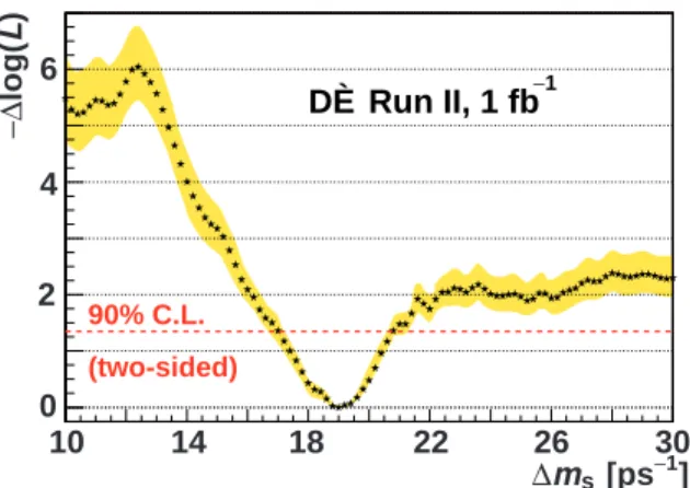
Figure 2 shows the value of −∆ log L as a function of ∆ms, indicating a favored value of 19 ps−1, while

vari-ation of − log L from the minimum indicates an oscil-lation frequency of 17 < ∆ms < 21 ps−1 at the 90%

C.L. The uncertainties are approximately Gaussian in-side this interval. The plateau of the likelihood curve shows the region where we do not have sufficient resolu-tion to measure an oscillaresolu-tion, and if the true value of

−∆ log( L ) 0 2 4 6 26 22 18 14 10 [ps ] s m ∆ 30−1 90% C.L. (two-sided) DØ Run II, 1 fb−1

FIG. 2: Value of −∆ log L as a function of ∆ms. Star symbols

do not include systematic uncertainties, and the shaded band represents the envelope of all log L scan curves due to different systematic uncertainties.

∆ms > 22 ps−1, our measured confidence interval does

not make any statement about the frequency. Using 100 parametrized MC samples with similar statistics, VPDL resolution, overall tagging performance, and sample com-position of the data sample, it was determined that for a true value of ∆ms= 19 ps−1, the probability was 15% for

measuring a value in the range 16 < ∆ms< 22 ps−1with

a −∆ log L lower by at least 1.9 than the corresponding value at ∆ms= 25 ps−1.

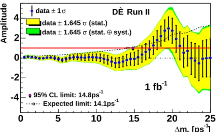
The amplitude method [16] was also used. Equation 1 was modified to include the oscillation amplitude A as an additional coefficient on the cos(∆ms· Kl/c) term. The

unbinned fit was repeated for fixed input values of ∆ms

and the fitted value of A and its uncertainty σA found

for each step, as shown in Fig. 3. At ∆ms = 19 ps−1

the measured data point deviates from the hypothesis A = 0 (A = 1) by 2.5 (1.6) standard deviations, cor-responding to a two-sided C.L. of 1% (10%), and is in agreement with the likelihood results. In the presence of a signal, however, it is more difficult to define a con-fidence interval using the amplitude than by examining the −∆ log L curve. Since, on average, these two meth-ods give the same results, we chose to quantify our ∆ms

interval using the likelihood curve.

Systematic uncertainties were addressed by varying in-puts, cut requirements, branching ratios, and pdf model-ing. The branching ratios were varied within known un-certainties [1] and large variations were taken for those not yet measured. The K-factor distributions were var-ied within uncertainties, using measured (or smoothed) instead of generated momenta in the MC simulation. The fractions of peaking and combinatorial backgrounds were varied within uncertainties. Uncertainties in the reflec-tion contribureflec-tion were considered. The funcreflec-tional form to determine the dilution D(dtag) was varied. The

life-time τB0

s was fixed to its world average value, and ∆Γs was allowed to be non-zero. The scale factors on the

sig-] -1 [ps s m ∆ 0 5 10 15 20 25 Amplitude -4 -2 0 2 4 (stat.) σ 1.645 ± data syst.) ⊕ (stat. σ 1.645 ± data σ 1 ± data -1 95% CL limit: 14.8ps -1 Expected limit: 14.1ps DØ Run II -1 1 fb FIG. 3: B0

s oscillation amplitude as a function of oscillation

frequency, ∆ms. The solid line shows the A = 1 axis for

reference. The dashed line shows the expected limit including both statistical and systematic uncertainties.

nal and background resolutions were varied within un-certainties, and typically generated the largest system-atic uncertainty in the region of interest. A separate scan of −∆ log L was taken for each variation, and the envelope of all such curves is indicated as the band in Fig. 2. The same systematic uncertainties were consid-ered for the amplitude method using the procedure of Ref. [16], and, when added in quadrature with the sta-tistical uncertainties, represent a small effect, as shown in Fig. 3. Taking these systematic uncertainties into account, we obtain from the amplitude method an ex-pected limit of 14.1 ps−1 and an observed lower limit of ∆ms > 14.8 ps−1 at the 95% C.L., consistent with the

likelihood scan.

The probability that B0

s- ¯Bs0 oscillations with the true

value of ∆ms > 22 ps−1 would give a −∆ log L

mini-mum in the range 16 < ∆ms < 22 ps−1 with a depth

of more than 1.7 with respect to the −∆ log L value at ∆ms= 25 ps−1, corresponding to our observation

includ-ing systematic uncertainties, was found to be (5.0±0.3)%. This range of ∆ms was chosen to encompass the world

average lower limit and the edge of our sensitive region. To determine this probability, an ensemble test using the data sample was performed by randomly assigning a fla-vor to each candidate while retaining all its other infor-mation, effectively simulating a B0

s oscillation with an

infinite frequency. Similar probabilities were found using ensembles of parametrized MC events.

In summary, a study of B0

s- ¯Bs0 oscillations was

per-formed using B0

s → µ+D−sX decays, where D−s → φπ−

and φ → K+_K−_{, an opposite-side flavor tagging}

algo-rithm, and an unbinned likelihood fit. The amplitude method gives an expected limit of 14.1 ps−1 _{and an}

ob-served lower limit of ∆ms > 14.8 ps−1 at the 95% C.L.

At ∆ms = 19 ps−1, the amplitude method yields a

re-sult that deviates from the hypothesis A = 0 (A = 1)

by 2.5 (1.6) standard deviations, corresponding to a two-sided C.L. of 1% (10%). The likelihood curve is well behaved near a preferred value of 19 ps−1 _{with a 90%}

C.L. interval of 17 < ∆ms < 21 ps−1, assuming

Gaus-sian uncertainties. The lower edge of the confidence level interval is near the world average 95% C.L. lower limit ∆ms > 16.6 ps−1 [2]. Ensemble tests indicate that if

∆ms lies above the sensitive region, i.e., above

approxi-mately 22 ps−1_{, there is a (5.0 ±0.3)% probability that it}

would produce a likelihood minimum similar to the one observed in the interval 16 < ∆ms < 22 ps−1. This is

the first report of a direct two-sided bound measured by a single experiment on the B0

s oscillation frequency.

We thank the staffs at Fermilab and collaborating in-stitutions, and acknowledge support from the DOE and NSF (USA); CEA and CNRS/IN2P3 (France); FASI, Rosatom and RFBR (Russia); CAPES, CNPq, FAPERJ, FAPESP and FUNDUNESP (Brazil); DAE and DST (India); Colciencias (Colombia); CONACyT (Mexico); KRF and KOSEF (Korea); CONICET and UBACyT (Argentina); FOM (The Netherlands); PPARC (United Kingdom); MSMT (Czech Republic); CRC Program, CFI, NSERC and WestGrid Project (Canada); BMBF and DFG (Germany); SFI (Ireland); The Swedish Re-search Council (Sweden); ReRe-search Corporation; Alexan-der von Humboldt Foundation; and the Marie Curie Pro-gram.

[*] On leave from IEP SAS Kosice, Slovakia.

[†] Visitor from Helsinki Institute of Physics, Helsinki, Fin-land.

[1] S. Eidelman et al., Phys. Lett. B 592, 1 (2004).

[2] E. Barberio et al. (Heavy Flavor Averaging Group), hep-ex/0603003. Note that we take ~ = c = 1, hence the units on ∆ms.

[3] J. Charles et al. (CKMfitter Group), Eur. Phys. J. C41, 1 (2005).

[4] M. Bona et al. (UTfit Collaboration), J. High Energy Phys. 07(2005) 028.

[5] Charge conjugate states are assumed throughout. [6] V. Abazov et al. (DØ Collaboration), physics/0507191

[Nucl. Instrum. Methods Phys. Res. Sect. A (to be pub-lished)].

[7] V.M. Abazov et al., Nucl. Instrum. Methods Phys. Res. Sect. A 552, 372 (2005).

[8] S. Catani et al., Phys. Lett. B 269, 432 (1991), “Durham” jets with the pT cut-off parameter set at

15 GeV/c.

[9] J. Abdallah et al. (DELPHI Collaboration), Eur. Phys. J. C 32, 185 (2004).

[10] G. Borisov, Nucl. Instrum. Methods Phys. Res. Sect. A 417, 384 (1998).

[11] V. Abazov et al. (DØ Collaboration), Phys. Rev. D (to be published); DØ Note 5029, available from http://www-d0.fnal.gov/Run2Physics/WWW

[12] T. Sj¨ostrand et al., Comput. Phys. Commun. 135, 238 (2001).

[13] D.J. Lange, Nucl. Instrum. Methods Phys. Res. Sect. A 462, 152 (2001).

[14] R. Brun and F. Carminati, CERN Program Library Long Writeup W5013 (unpublished).

[15] G. Borisov and C. Mariotti, Nucl. Instrum. Methods Phys. Res. Sect. A 372, 181 (1996).

[16] H.G. Moser and A. Roussarie, Nucl. Instrum. Methods Phys. Res. Sect. A 384, 491 (1997).