An analogue for motor-vehicle vibration

AN ANALOGUE

FOR MOTOR-VEHICLE VIBRATION

by

0. Mauri I. Kurki-Suonio

B.S. in M.E. Finland's Institute of Technology

'

''

~~~~~~~1948

Submitted to the Department of Mechanical gineering

on May 16, 1952 in partial fulfillment

of the requirements for the degree of

%.

MASTER OF SCIENCE

':~>~~~~

rfrom

the

Massachusetts Institute of Technology

1952

'... ,.

Signature

of

Author

...

...

.

'*

S

_.

.

* *

!%i:

Department of Mechanical Eagineering, May 16, 1952

/9/

Professor in Charge of Research"

Chairman of Departmental

Committee on Graduate Students ..

C,

~

:

A~~~~~~~~~~~~~~~~~~~~~~~~~~~~~~~~~~~~~~~~~~~~~~~~~I

II

I i

bit,~~~~~~~~~~~~~~~~~~~~~~~~~~~~~~~~~~~~~~~~~~~~~~~~~~~~~~~~~~~~~~~~~~~~~~~~~~~~~~~~~~~~~~

O%9

OCT 7 1q52

by

O. Mauri I. Eurki-Suonio

Submitted to the Department of Mechanical

Eagineering on May 16, 1952 in partial

fulfillment of the requirements for the

A motor-vehicle with its springs and pneumatic

tires forms a very complicated vibrational

system. Although

the direct mathematical solution may be obtained for

systems of one or two degrees of freedom, the problem

of the complete vehicle is best solved experimentally.

The purpose of this thesis was to design and

build a mechanical analogue for motor-vehicle vibration.

It consists of a body and two unsprung masses. The body

is suspended by springs from the two masses which in

turn are suspended by stiff springs representing the

...

tires.

-: -

~~In

designing a model it is necessary to retain

certain dimensionless uantities which are determined

through the methods of dimensional analysis. The

wheel-base of the model was chosen to be approximately one

fifth of that of the average American car. The spring

and tire stiffness

and the weight distribution

may be

electro-makes use of the fact that the force opposing the motion

of a conductor in a magnetic field is proportional to

the velocity of the conductor. By changing the exciting

current in the electromagnet which produces the magnetic

field, the amount of damping may be controlled.

With a

recording device the apparatus shows the motion of the

body directly and can be conveniently used for study on

problems of motor-vehicle vibration as well as

demons-tration pmrposes.

' Thesis supervisor:

C. ayette Taylor

Title: Professor of Automotive

The writer wishes to take this opportunity to express his sincere appreciation to Professor

G. F. aylor for his constant interest, kind

encour-agement, and helpful advice throughout his

super-vision of this thesis. Other aid I am happy to

acknowledge came fram Professor J. E. Forbes. His

suggestions were an invaluable aid in designing

the electromagnetic damper. The kind interest taken

by all members of the staff of Sloan Automotive

Laboratory has done much to make this thesis both

Page

I.

Introductin ... 1

II. Mathematical Consideration

.

. . . 3

1. The Single Mass System

...

3

2. The Two Mass System . . . 6

3. The Body with Distributed Mass . . . 9

4. The Complete Vehicle . . . .12

III. Similitude of Vibration Systems . . . 17

1. Dimensional Analysis

...

17

2. Use of Differential Equations . . . . 20

IV.

Description

of the Analogue

. . . 23

1. General . . .

.

. 23

2. Weight Distribution . . . 24

3. Springs . . .

..

. . . 26

4.

The

Driving

Mechanism

. .

. . .

..30

5. The Recording Mechanism . . . 30

V. Electromagnetic Damper . . .. . . 31

1. General Theory . . ... . . . 31

2. Design

of the Magnet

. . . .

.

.

34

VI. Test Results . . .

..

. . . . 42

VII. Conclusion . . . . . . . . . . . . . . . 53

The purpose of a motor-vehicle suspension is

to protect the vehicle and the passengers or load from

the road shocks. The suspension problem is very important

and

it has been the subject

of extensive

research

both

in this country and Earope (References 1...10).

Dr. Haleys

thesis on vibrational characteristics of automotive

suspensions which includes a large bibliography, may be

mentiozndhere as a study made previously at Massachusetts

Institute

of Technology

Unfortunately, the motor-vehicle with its

springs and pneumatic tires forms a very complicated

system. Even when only vertical

displacements are

considered and the effect of seat cushioning is neglected,

the system still

has seven degrees of freedom.

Mr. P.E. Mercier proposed a solution for the

vibration problem of the complete vehicle in his article

on vehicle suspensions 12 He considered a system

consisting a body and four wheel masses. He assumed also some kind of interaction between different wheels,

i.e. the load of the suspension member corresponding to

one wheel caused by the motion of another.

In order to simplify the mathematical procedure

Mercier assumed complete symmuetry

of the vehicle. Further

ing that when elastic characteristics are rationally determined the required degree of damping is low. It is

true that damping has very little effect on the frequency

of the vibration. However, it significantly affects the

amplitude, especially with steady-state disturbance at

resonance frequency when damping is essential.

In this thesis the problem of vehicle vibration

is

_{considered using a mechanical analogue.}

The

problem

has been simplified by neglecting the rotations of the

body and the two axles about the longitudinal axis of the vehicle. These motions may be studied separately.

In other words, motions are considered only in the

vertical plane parallel to the direction of travel of

the vehicle. The number of degrees of freedom is thus

reduced to

four,

namely the '"bouncing" and "pitching"

of the body and the up-and-down motions of the two

axle s.

II: MATHVL TICAL CONSIDERPTIONi 1 11. 1 1 ' II Ill~~~~~~~~~~~~~~~~~~~~~.

The Single Mass Sstem

To start with the simpldi;t

kind of vibration problem let us

consider frst

the single mass system

[ T

as shown in Fig. 1. The motion is

determined by a second order linear

'

differential

equation. By simple

calculations the complete solution

for free vibrations can always be .. - : lg:. .

found 13 and is of the form:

K,

= A, es, t * e

where

4x,

(1)

-+

and

A

1

and

A

2

are arbitrary

constants which depend on

the initial conditions.

The values for s can be real or complex. In the former case the motion is not vibration but an exponential

curve to the equilibrium position. The smallest amount of damping for which this occurs is

(2)

This is called the critical damping. The damping coefficient is usually expressed in fractions of the critical value.

Usinig the fact that the natural undamped frequency is

the solution of the motion can be expressed in another,

more convenient form:

x=A

e

C,

s.

(4)

The coefficient A and the phase angle

depend again on the initial conditions. The value

.~V~JL

.,

is called the

damped

natural frequency. We see that a

reasonable amount of damping has very small effect on

the natural frequency. A damping coefficient which is

half of the critical value reduces the natural frequency

only by 13.4 per cent.

The solution for a forced vibration is also

found if the forcing function (the

form

of the road

surface) and the initial conditions are knlown.A

road

surface of sinusoidal form may be defined as a function

of time thus:

x%

- ao

((-

dt tJ

5)

The initial vertical displacement and velocity of the mass are assumed to be zero. The following

expression is then found for the motion of the mass as a function of time:

A7

olA,

4>A

e

4 O.' (6)

where the coefficients

A

1

and A

2

and the phase angles

,

and O

are functions of damping ratio and frequency

ratio:

+~~~~

A,

_~

+

_

¢.

/Xtcj

r~,~'(Q,:"/:~' _{2 %. (} L%~-.)."

3'1,)=

2..

-

-

2T>.t- L,,.

c/~3

_{1 . _..}

The motion is described by three terms, namely

a constant, a sinusoidal term varying at the forcing

frequency of the system. The third tenm decreases ver

rapidly and some time after the disturbance has begun the system is said to be in steady-state vibration, because the motion is purely periodic. Coefficient A₁

is the ratio of the amplitude of the motion to the amplitude of the road surface. If it is plotted as function of frequency ratio for different damping ratios the well-known chart of Fig. 2 is obtained.

The Two Mass System

For the two mass system

with the notations of Fig. the differential equations are:

Fig. 5

rn,,,c(?,,-,.)

+ ,Cx,-:)-

mr,

c4-,) +

k x

-x.

x

0x-

(8)

The natural undamped frequencies of the system

are ound to be the roots of the equation 14

whioh

ar+

+~~~~

+

k

which are:

<

~ ~

~~.

.

Hat

_

I r= .

'+Cb

-

-

tt

21 03.

3.0

}

k

2.0

!s i I .t

,0

, . ' I I - - ~ I . .

. ..

2.o i t

L

, .. .

,n

For the motor-vehicle k>k and ml$ m2. Then

the natural frequencies are approximately:

;;L

ap

=

k' t

i

1

(10)

Assuming again a road surface of the form:

and that the initial displacements and velocities are zero, the method of Laplace transform 15 can be applied for solving the problem. The Laplace transforms of x and x₂ are found to be:

X -_""" -t. .C -. , k*

_

~~a.

4

₄

)t~

Kn(

f(PI'+P +

)P(3

+^J<

4- CkZ+

AdL,

For the inverse transform it is necessary to find the roots of the fourth order polynomial in the denominator. If the system is oscillatory the roots are all complex and of the form:

p

_ r

!

+

i< 3

It is possible to find these roots if the

numerical values of the coefficients are given. Dr. Haley

The general solution as algebraic function of the coefficients is not obtainable as in the case of one degree of freedom.

The steady-state

solution may be obtained

quite

easily

in terms of the parameters of the system

without evaluation

of the roots

of

the fourth

order

polynomial. This is accomplished by assuming that the

solutions are of the form:

XI

Ate

X=

'

l(12)

If these are substituted into (8) and the equations are solved for and x2, the amplitude

ratios are found to be:

1'1 = 0 iXt.. 0

{kik At

.Qt

Z~

a . - I $ . ^ - , 1. ?

3

IL+I& k

4

ao

It 1-4

+ ( kz Adk 1

-

/. W 4- la.j 1cW_ (13) .i _{I (kxlteI ih} .. . . _ . _L

J

.

kI

_ka,

JLf

The first part of the denominator is the same

as

the equation for determining the natural frequencies.

This is clear because without dmping the amplitude goes to infinity if the forcing frequency is the same as the

natural frequency of the system.

I

z i

11 I

The Bdy with Distributed Mass

As next step let us consider a body with distributed mass ad two parallel springs. This is

also a system of two degrees of freedom.

Fig. 4.

With the notations of Fig. 4 the differential

equations of the system are:

t r

..

m

- 2.- A

X

,

~t

*, XI

*e

m "~L

j, = c

(14)

.1h 4rL

..

" It

n

rx

ry,',

.t

=-The natural undamped frequencies are the roots of the equation:

L4 c,."+ r k, .rL)L + + L k tC.,

(15)

A particularly interesting case occurs when

the ratio I S., i2. a II a z6

which is called the mass coupling, is zero. Then the set of differential equations (14) reduces to two separate equations and the mnotions of and ₂ are independent of each other. The natural frequencies are then simply:

(16)

Another exception is the case hen

i~~~~~~~

or spring constants are proportional to the wheel

loadings. This means that the taticdeflections in

front and rear are equal. Then the natural motions are

pure up and down motions parallel to itself

and rocking

about the center of gravity. The natural frequencies

of these motions are:

!~~~~~

tA

(17)

*~~~~~~~~~A

-

i,

,+ ka.L,6

If mass coupling is also zero these frequencies

are equal.

Let us assume that the initial

displacements

and velocities are zero and the exciting motion under the

wheel 1 has the same form as previously:

The Laplace transformsi of the motions are:

X,(?) =

X"(,P) =

1

2.WL

L4Ia'

t(

-)(

4

jL

+7

where the constants a

1

. ... a

7

are:

Ikcg t*+ r c , k-

*

--CZ, -2c, 4,x 27 = Mr a = C' if?. jV# I i tL- *

¢,

I

+ r%

,,,&.

c, C. l, X. ~, t,2+r ~

For the inverse transform the roots of the

fourth order polynomial in the denominator are required.

The amplitudes for steadystate

bration are found

without evaluation of the roots through a method

used previously for the two mass system and they are:

Xs

[-

0(alq)

(a\

*g)Aawhr

7)

t4lagt

L(Q+

*)

_ tf~~~~~~~~~~~~~~ae

jx

J

(18)

1L-%

( L

I WA S4 'S - % 4

n,74j +

I .

B

Os j

r -&

14 ₁₁ 1W, I

-k

a7 IL 4-

I

.0

-a EM I- 4,) a to' 2. -L 19)I

The omplete Vehicle

Fig. 5.

The vibrational system of the complete vehicle as chosen for this study is shown in Fig. 5. It is a

combination of the two previous cases and has four

degrees of freedom. The following coordinates are used: x = rise of the body at center of gravity

= rotation of the body about center of

gravity (positive counterclockwise)

x rise of the body at wheel 1

x = t "it t 2

terms of

U = " of the mass m

4=

" " m2

X$ = " of the ground under wheel 1'

x

=

"

"

"

2

The coordinates x and '7 can be expressed in

x

1

and x2:

L5t

4-~~~A

Let

1

and F

2

be the algebraic sum of the

spring and damping

forces at front and rear respectively.

From the balance of forces and moments acting on the

body

we get:

- M + +

2s

-Mrz8

+

-

(21)

Substituting the values for x and from (20)

and the values for F₁ and F₂:

P =- c, (,

-Z)

-k,

,-

X)

(22)

F

2

.

C =

4

-)) 2 2 Xa

we get the differential equations for the motion of the

body:

M

Z~

3

*

'

M

--

x,

c,

,-~), k,cx,x1

+

o

(23)

\

jxs ,-

+

C (%-

k,4)

+ kiL,^

The differential equations for the unsprung masses are found to be:

nM

, .-

(k,

)-x ,-i

x)

x2-

X

-(24)

Let

_{us consider a sinusoidal forcing function}

which hits the rear wheel

/

v.

later than the front

wheel:

X -

I

(*j

& o,

Ij

(i

-

(25)

If all the velocities and displacements are

zero for t=O, the Laplace transforms of the equations

(23) and (24) are:

M

t+ r

X-t *

rZ

M

'- L LM L-' --y--

F.A

L . - r .

+

r

k3 x a

k a +

(26)

Jp2g. .m (F Fx-.:/i

After elimination of 23and

i4:

P 4 ,. X + I

L4~

i l' L~~~~~1

0_,@-+ rt

P3f(

f

k

!

,L

j

-'

*

tm

1,, jL

j P

'K

P

~,

F4

11

~

A I

=- C2. + "7t ,/-k

F

4-I!pE*.

J,1jpL

+ G -t wq L

sV

t

-L+ rL ! La,

o

FL+

TW40 f

(27)

r4

4. ,.r ,> C * F

F3

L

t

+x

F

(. e 7, + rr~rr~-Up - IU j.l 'A j

= a ( -E~

fC~pl~l-j4-) Uk - :Wa " C k i L i el F k fmf Q, j

These equations can be solved for

1

by the use of determinants. The denoininator ill be:

4-.

1

+

c

,)

where the coefficients are:

I

4',

A,

k

~L

7 =

( A It. '-

t 2-j

+'

A

,kt&

'O

,~

t

/ ,4 _-raX

._ a.

i. 'y

g J-AL k + )

+

A.

I

&4

.

f

ic

)"# 2

k

4.L'i rbi *-C Cx I. en , ;6,

i J

4- (A₁

; ;,Y

- w tV

K

+ -z ( . 'I ,+ L-Al = A. k M

kA,

5 ,

%.,

I

.

-

V'

₁

s,;+ .t)1~v '

2. MAC. ik A

IA

}

A r, ¥"v111.~C =A t C., !^t- kA 1 t ) A M. . __ t~~~~rb a-s F-t 'It m -,M I' + _{C - .'} W. *M . A - fa , I~ ` s . '-

-'k = -~it

j

A t = It

,., - -_1.% anu x2

(28;

_ -- (t , C, 'C A-2 X.. =

~

~x

+ 51 Ssk.3,~.~A

~4 i&

)

%.,

* k'

~~

1

-

t --

+ -k-%

i, f-4 Lzk S t 11 W.A _{W.% -* kA '} -1--l"S -- ") M .,, -4. (A\ _+' -2.

- (A -,..

R) K.

_4 .4- X 4 PR '. l.A

~t

IL

FQT

inverse transform it is necessary to find

the roots of the eighth order polynomial in p. If the

numerical values of the coefficients are known, the roots

can be found using-Graeffe 's method 16, but it is quite

too laborous for any practical purposes. Therefore the

mathematical solution of the vibration problem of

the

vehicle is not btainable. The only way to find the

III. SIMILITUDE OF VIBRATION SYSTEMS

Dimensional

Anysi

Dimensional analysis treats the general forms

of equations that describe natural phenomena. Applications

of dimensional analysis abound in nearly all fields of

engineering, particularly in fluid mechanics and

heat-transfer theory 17. If experimental methods are to be

applied the scope of the results can frequently be

increased through the use of dimensional analysis.

In designing a model of a vibrating system it is necessary

to retain certain dimensionless

quantities just as in any

other model making.

The procedure in the application of dimensional

analysis is first to list the various fundamental physical

factors or dimensions

which

enter into the problem. These

quantities

can be determined by examining the differential

equations of the simpler problems. These and their

fundamental units are:

1.

Mass

-

s-

W/g

FT2/L

2. Spring constant -

k

F/L

3. Damping constant

-

c

FT/L

4. Natural frequency -

1/T

5.

Forced frequency -

1/T

6. Displacement

-

x

L

7.

heelbase

-

i

L

8. Moment of inertia - I FT2L

The time might be considered but it does not seem necessary because it is the reciprocal of the frequency. The force does not enter in because except inertia, spring, and damping forces no external forces are acting in the system.

The terms involve three fundamental units,

F, T, and . The number of 7r functions that may be

determined is the number of factors (8) minus the number

of fudmental units (3), or five yt functions. Among tha variables listed three are selected which contain

all three of the fundamental dimensions among them.

These are the mass, the wheelbase, and the natural

frequency. These are set down vwith one of the other

variables written after them. If

,

/,

and

t

are arbitrary

powers to be

assigned

to the three

quantities selected, then the dimensional equations

can be written as:

r.

"

rr,

4't

m

(<~

±~1

QL

I":, ,FT

.

L..

r

J3t a)

T"

r (29)T

(29)

"r

i

>,*/

i")4~

_

,

...

i

J77 ; Ai 43lj_~ _ ok 1· a STT

The sum of the exponents for each of the

fundamental units must be zero. Therefore for

rT,:

C'(1- + I _{(Powers of force, F)}

(Powers of time, T)

- <( +- ,(j = _{(Powers of Length, L)}

When these equations are solved simultaneuusly the values of the exponents are:

Aq = -I

t =

so that the first imensionless fnction is

so that the first dimensionless function

YA

is

The remaining functions may be evaluated in

a like manner:

C I

-3

e

_(1'Al 4.. /

( = .t i

a

If these five dimensionless quantities for one system are equal to the respective quantities of another

Use of Differential Equations

For the complete vehicle which has three

masses, four different spring constants,

and

two

damping constants, the dimensional analysis approach

is not sufficient. More definite method is changing

variables in the differential equations to

dimension-less form.

The differential

equations for the complete

vehicle are, combining (23), (24), and (25):

-. + X i, I - .

Zz.l

7 .X +

a+M*TL A

-

+

..

;^-+x)

4

k

,t

-X E

(30)

lh, <Xg - $ jY,- tj~ k, X -t Ck,+ z 3 '

,

+) C-

If a change of variables is made using

(31)

When the dimensionless terms are differentiated, the results are:

L l = A__T

'~

,)

-

_{z^_t}

S ='

_g

£ : J._T'

These derivatives are substituted in the

original equations:

2""+ +, L

g W

tl

L&{c

-xzK

+ M

I

"T Y4)

Ar

z-4

-H. 1 Luf ~ u(32)

t",t:-

_{r r~~~~~~lr}

I

_rrr~~~A;*

(X-i)_

<sc<

(k

1

.k

4

_Ot

L

k

.L-.(w&-i7

Uiw-

Since X and T are dimensionless, their

derivatives are dimensionless. If each equation is

divided

by

the

coefficient

of the second derivative,

it makes all terms dimensionless:

.... _ (.C

L

_ t

z

_j/.

,, &(3y) XEl ,+ ( r 1

,

.

kkt

<A ,

W3

1---

- ,

_{-I~r, A t}

n

₎

13

-- -

L

_{- , -} - -/ A : . k* + WC

If these quantities are equal in two systems

also their ratios are equal. This way following quantities

may be determined:

, ',

L2 '

The

_{final conditions that two vibration systems}

are- similar, are that following dimensionless constants

in one system are equal to corresponding constants in

another system:

- Weight

distribution

2.

r,%,

.

3.

c, L

5.

~ '2o

i

6. o!,

L

7.

8.&, B

9. a.

10.

!&

j

-

Mass coupling

-

Relative damping

- Static deflection

-

Spring coupling

- Damping coupling

- Relative weight of unsprung mass

- Relative tire stiffness

- Amplitude/wheelbase ratio,

- Frequency ratio

- The ratio of driving speed to

the product of natural frequency

and the wheelbase

1*. l/?

IV. DESCRIPTION OF THE ANALOGUE

General

The main purpose of the analogue was the use

for demonstration of vibrational characteristics of the

motor-vehicle. It was therefore quite natural to think it first as a small-scale model of the actual vehicle

as shown in Fig. 7,

using compressxon

springs in the place

of springs and tires. However, the guidance

needed in this type

of roalab wrOlA

involve too much friction and the application of road

disturbance would not be convenient.

For smaller friction and easier guidance the

whole system was turned upside down as shown in Fig. 8.

Altnougn a alttle

more imagination is

needed in order to

understand that this

represent an

auto-mobile, it was found

very succesful. Fig. 8.

----No guides are needed to prevent other than vertical motions because the system is always stabile in the field of gravity. The friction is thus reduced to a

minimum. Further the road disturbance is easily

rep-resented by a single rotating

cam

which

affects

both

front and rear wheels through rocker arms.

Weight Distribution

The wheelbase of

the

analogue was chosen to

be

24 inches which is approximately one fifth of

the

wheelbase of the average American car. The weight of

the analogue does not need to be proportional to the

third power of the linear ratio as for some other models,

because the laws of similitude do not include any

relation between the mass and the legth in this case.

It was desired to have a large range of weight

distribution.

Therefore the "chassis" was made of

l"

duralumium bar, 40" long, which weighed only 1.01 lb.

Four movable steel weights were made weighing 1.10 lb

each. The heaviest part of the analogue are the

electro-magnetic dampers which will be described later.

They

weigh

3.38

lb

each.

The weight of the whole body is

Chassis 1 x 1.01 lb = 1.01 lb

Weights

4 x

1.10

"

4.40

Dampers 2 x 3.38 t = 6.76" 12.17 lb

i

--

--The moment of inertia of the chassis and the

dampers is:

vL" t.olh4oL _

= Ix

l I 'fL 7 lb,"

I

0

Ibb-iJ1'

The variation in the

moment

of the inertia is

due to the change of position

of the

weights.

The

minimum

is obtained when all four wights are in the center of the

bar, and _{the maximam when they are at} both ends of the bar:

J.,J

=

4.

.

I.os

Ib...

The minimum

and the mmm

radii of gyration

of the body are:

r/

_r,

'lo+ is-as

_rV

₌

.j

_.

p.

The minimum and the maximum mass coupling at

symmetrical weight distribution

are:

r',;t

I1.

'

'

_____

-

/- = AZ.

to x J-ai '

The mass coupling can be varied in larger range

than in actual vehicle. In order to get zero mass coupling

(r2/1, - 1) at symmetrical weight distribution the

moment of inertia must be equal to the mass multiplied

by square of the half of the wheelbase:

_Ti ma be otn= h Ib .17 a

This may be obtained so that two weights are

left

in the center and two are put 17.075" from the center. This

distance is marked on the bar as well as the center for

easier weight installation.

Springs

Because of the large

size of the damper

it

was

found more convenient to use a set of two parallel springs

between the body and the unsprung masses instead of a

single spring.

n. ,l-

' P:'-nn, -'H_ . 4,'-'P'iI -enlrr.

w

t~'i'h+t

distributions a large number of springs of different rates was needed. The maxmum and minimum spring loads

which were half of corresponding

axle

loads,

were

estim-ated 4 lb and 2 lb. The static deflections between 4 in.

and 8 in. were desired corresponding the frequencies

94...66 cycles per minute. The maximum

and minimum spring

rates were then found:

- - -I

... . .. . . -. - . -.- .. . - --- - -L.-L~L YUL~-LI

k

- = I /.

kis

; _

-

8

.

,5

Ib/n.

Etension type springs were ordered from

Hardware Products Company, Boston'. These are made of

high quality spring steel and have initial tension

which makes the actual static deflection smaller than

what is the effective deflection. A table of these

springs and their properties is given below.

Outside diameter in.

3/8

1/2

Wire diameter

in.

w 031 047 062 047 062 094

Max. load lb.

4-2

15.

35.

11.

25.

85.

Max.

extension

in.

3.4 1.2

.7

2.4 1.2

4

i

Initial tension lb.

.9

3.0 7.0j 2.2 5.0 17.

Spring rate lb/in.

1.0

9.6 43. 3.7 16. 153

_ _ _ _ _ ~ ~~~~~~~~~~~~~~~~ _ _

The figures for maximum

extension and spring

rate are for springs one inch long. The maximum

load

and initial tension remain constant for any length.

In order to keep the weight and the free length

of the springs as small as possible the suspension springs

were made 3/8" outside diameter .031" wire diameter.

The maximum

load for this spring is just above the

maximum required.

For "tire" spring the load varies between 4

and 8 lb. Statie

deflections

from .8" to

'.4"

were

wanted

because

the

_{natural frequency of tires is approximately}

ten times that of the suspension springs. Spring rates are then:

=

8

=

o

Ib/,

kM;^

=

i -

4

A

=

-

.-A set of springs of seven different lengths

were ordered for both purposes. All springs were

care-fully tested and the actual spring rates are listed below:

Suspension springs

3/8

x

.031

V Rate 5 Leength I 1" 3/2" Rate i 1.26

.833

Tire springs

3/8

x .47

Length

4 tt Vt'

1"

i

-t '.

' J

/

-/

5"

.410

.

,I

3 .410 1 lAtt Rate

13.8

10.0

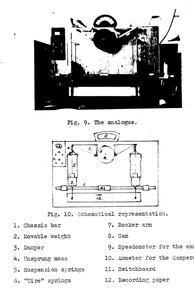
q_ LLR i . 9 1 6.90 .5345 i a 6.13 i 41" .298 2' 5.25 1, I 2" .605 424" -LL C _rr~-RD--a~lu~nu.·urw_.S vrrnr·~~rl r _ ._~~~~~~~~~I Pn-nD----,.-- im

Fig. 9. The analogue.

:z

I?

\

fz

Fig. 10. Schema-tical 1. Chassis bar 7. 2. Movable weight 8. 3. Damper 9. 4. Unsprung mass 10. 5 . Suspension springs 11. "T. "Tire" springs 12.

repre sent ation. Rocker arm

Cam

Speedometer for the cam

Ammeter for the dampers Switchboard Recording paper L

- 1

I_ __I __I I I I I I I I i I I II I I I I I

The Driving Mechanism

For driving the cam which produces the road shocks a variable speed electric motor is used. Through a reduction gear the speed scale is O...400 rpm, but

30 rpm is practically the lowest speed possible. The relation between the cam rpm and the vehicle speed in mph whish has to be represented, may be found through following reasoning. During one half of cam revolution the analogue "travels" a distance equal to the wheelbase. At n rpm the distance traveled in one hour is

60 x

n 21

If the wheelbase is measured in feet, rpm

scale must be multiplied

by

120O

d=

.0227"1

in order to convert the speed into mph. For an average car of 10 feet wheelbase this coefficient is .227.

The Recording Mechanism

For measuring the amplitude of the motion a

recording mechanism is provided which uses regular 3"

iade adding machine tape. The tape is driven by an

electric

motor through a three-speed gearbox. The speeds

for the tape are .3",

1.0",

and 5.0" per second.

_~~~~~~~~~~~~~~~~~~~~~--v. ELECTROmGNETIC DAiPER

General Theory

If a conductor moves in a magnetic field an

electromotive force is induced in the conductor. The

electromotive force causes a current which in turn causes a force opposing the motion of the conductor.

The force is proportional to the magnetic flux density

and the relative

velocity

of

the

conductor

with

respect

to the field.

This phenominon occurs in so called

eddy-current brakes used in laboratories to measure the

mechanical output of a motor. It may be succesfully

applied to represent an automotive shock absorber. It is ideal for this purpose because the damping is linear,

i.e. proportional to the first power of the velocity.

In a fluid dashpot there is always in addition to the

linear viscous damping more or less hydrodynamic damping

which is proportional to the square of the velocity.

Tiner ,m1in"

__

i

irtla.l not

---

nnl

-d

fn-r the simnlicity

-- _ - J

of

--mathematical treatment but also from comfort standpoint.

The control of an electromagnetic

damper is

also easier than in a fluid damper.

This

is accomplished

by changing the exciting current in the electromagnet.

The only drawback is considerably heavier eight.

It was figured,

however, that even when one half of the

weight

_{of the body would be concentrated at the places of}

spring attachment in form of dampers, the desired range

of weight distribtuion

would still

be obtained by

using

light aluminium

bar for chassis and heavier movable weights.

This

gave

for

each damper an approximate weight of three

pounds.

In order to use the material most efficiently a round magnet as shown in Fig. 11, was suggested.

A cylinder of non-magnetic

material of high conductivity

moves up and down in the

circular

air gap. The magnet

i

o 4" o 4 9 M o -- - - -- I -

-na

s o

e aacnea

o

une

body and the moving cylinder

to the axle mass. Otherwise

tne unsprung mass would

become too large.

Fig. ll.

If the cylinder moves with a velocity v in

a magnetic field which has flux density B, the

electro-- . . .1

-QVlyO`ube

IO=f1TlaU71

n

1,11U

U

1US:(34)

it

E

=4~

2 2

t </ X

,

(34)

- = .5-~~~~~~~~~~~~~~~~_

u-i-;--- c--u-- -- r-- -Llrr

-The resistance of the piece of the cylinder

in

the air gap is in ohms:

- = (35)

where

~

is the resistivity

of the material (

for

copper

V =

6.79 x

10-7ohm

in.)

and b and

are the dimensions

of the cross section of the air gap. Electric current in

the cylinder is the electromotive force divided byy the resistance:

E -- = -

--I

=tIO

(36)

The force which opposes the motion of the cylinder is proportional to the current, flux density, and the legth of the conductor:

F =

f

I ld,,,

3

(37)

f is proportionality factor which das the value one when force is measured in newtons, flux density in webers/m2, current in amperes, and the length in meters. If the English system is used has to be calculated:

1 newton = .224 lb

i

weber/m

2

_{= 64500 lines/sq.in.}

1 meter = 39.37 in.

.22500 x

597

8.83 x 10- 8

By substituting the expression for current (36)

into (37) and using the Eglish units we get:

F

-

_8.83

o

-

_Lb

₍₃₈₎

The damping coefficient is equal to the force divided by the velocity:

F

-c

8.t3A

b 4

Tdn

(39)

Where: c = damping coefficient (lb.sec/in. )

q

resistivity of the material (ohm in.)

B flux density (lines/sq.in.)

b

=

height of the air gap (in.)

=

length of the air gap (in.)

$d mean diameter of the air gap (in.)

Design of the Magnet

If certain damping coefficient is desired, the

flux density required in the air gap is found from (39):

73z

/

C-(40)

If leakage is neglected the total flux in the air gap is equal to the flux in the core

A4B,

=-Ac

(41)

from which:

(42)

35

In order to reduce the number of variables in

the expression for Ba (40) the following step is made:

M

=

_

4

X

(43)

B)a 8.3$.Io'0 J d ; E

Magnetic field intensity in the air gap is

fK

, ,,

~

(44)

where i_{o 0} is the permeability of free space. If B_a is

measured in liner/sq.in. and Ea in amp.turns/in. then

it has the value

)l

3.192

The magnetomotive force reqired is

F,.i -

, ,.

c

., -

14

(45)

where is the path of the lines in the core. In the

first approximation the path from the inner core to the

outer core may be neglected. If the height of the core

is h and the value for

K

a

is substituted:

= _.,,.-"

(46)

o

aci

4

tI 2

(U)

The cross sectional area available for the coil:

A

5

Y

h

( -

-

6

)

(47)

The number of ampere turns which can be safely

used is:

N

I

=

C A

C

h (dm

-

di

-

)

(48)

-Cs is the safety carrying capasity of the wire

For small size ire in confined spaces it is approximate:

Cs = 2000 amp/sg.in.

The magnetomotive force is equal to the number of ampereturns:

A4C

, )LV L - L j . _

,

ly:

j.AI, aI0 - '"*T. y r . ' M -- n -c-,

-

(49)

8.1 1- 4)"O

Ir Al

L

t~,

from which h may solved:

4 qc,

_f

_rew

For certain value of core diameter this

expression has a minimum. This is found by differentiating

(50) with respect to

di

_{and setting that equal to zero.}

The optimum core diameter will be:

(51)

The magnetizing curve for cold rolled steel is shown in Fig. 1218In order to use the material efficiently

rather high flux density is desired. Corresponding

to the

assumed

maximum

flux density 120 kilolines/sq.in. the

maximum

field intensity is found by interpolation:

gK - 300 amp.tumns/in.

The length of the air gap was assumed 3/32"

and the mean diameter 2" because this size of copper tube

for the damper cylinder was available. The optimum core

diameter can then be calculated:

C 0c C ac, c c :3 0 E <c IC o C .C

-: o

C N

_{c Q}

L left O_{Q c} C

c

o

C 0

a

c

Cs ct c 0 CI L - * -m

300

3

-

0.875

in.

Corresponding value for h is found from eq.(51)

h

2.86 in.

Because in calculation of the lenugth of the path in the core the horizontal part was neglected the

total

height of the magnet was designed

2SL".

The

height

of the air gap was assumed /4".

The magnetizing curve for the magnet can be

plotted

be means of Fig. 12 and equation (45) which is

after necessary calculations:

Fm 11.25 Bc + 57 2

K

c

(52)

The damping coefficient c may be determined

as

function

of magnetomotive

force

by using equation

(39)

which is after calculations:(B

c

in kilolines/sq.in.)

c = .187 (B /100)2

_c

₍₅₃₎

The calculated values for Fm and c are in the

table below and _the damping coefficient vs. magnetomotive

force is plotted in Fig. 13.

Fm

ki lolines/in amp. turns/in amp. turns

20 40

60

70

80

90

100

110

120

4

6

9

12

16

23

40

100 300

248

484

727

356

992

1145

1354

1810 3066 C lb. sec/in. .0075

.0300

.0673 .0916

.1196

.1514 .1870

.2265

.2690 -l ;:,

q)a CL 3 .) o

u

-r A v a

_{A._}

> Irj_{_ _} m Ed W :> -A

L

E C

a

0 0 c C C C. 0 C

r

I-.0 I, 10.

0

_{to 0~}C I j i i I II I i i I I I 11"I iI I I I i I I i I I i i i i I I i i I I Ii . _ _ ~m C [SP

The critical damping coefficient for average

axle load (6 lb.) and spring rate (1 lb/in.) of the

analogue is

The number of ampere turns which gives this amount of damping is 2600 according to Fig. 13.

For coil it was suggested to use wire No 20, which specifications are 19:

Diameter 31.96 mils Area 1096 circ.mils

Resi stance 0.672 ohm/in3

The volume of the

coil is (Fig. 14):

v-J i = 5.1

in

.,

Resistance:

k

= 5

^

.t

0. ,'7 =

S

.2z-3

Z• ,

Fig. 14.

When the coil was made there were 14 layers,

55

turns

in

each, which means 770 turns total.

In order

to obtain critical damping coefficient the current must be:

I

2600

6= 3

.

38

A

N

77o

The voltage required is:

E = R I = 3.425 3.38 = 11.6 V

The maximum current is a little high for safety

carrying capasity of the rire. The cross section of the

I -. 11 71 l

-I

wire is only 292 circular mils per ampere when at least

500 is recommended in Radio Engineers Handbook. Because

the maximum

_{current is used only for short periods, this}

considered satisfactory. It was found that it did not

cause any damage even when the maximum current was left

on for several minutes.

In order to keep friction as small as possible only one wire was connected to each damper. The other terminal is connected to "ground" where the current is

1

t 'n A +4iro Is -nr r r; ncl w"1 r. n n- ^ 1 rr ^ ^I' C D4S -n

Xc s C;CLVL W44L6w 5"UF++ LL":; U APEX LWU LUV'UO L-=

used for controlling the current, one for the total

current

and

_{another for the ratio between the dampers.}

The wiring diagram of the damping system is shown in Fig.15.

I _i kI

I~~~~~~~~

ie

I

VI. TEST RESULTS

For using the analogue it is necessary to find

the relation between exciting current and damping

coef-ficient. The direct measuring of the damping force is

difficult

but

it can be conveniently

determined by

examining free or steady-state vibrations.

Free Vibrations

The rate of diminishing of free vibrations depends on the damping. The relation is shown in Fig. 16 where the ratio of successive half-cycle amplitudes is plotted against relative damping coefficient 20

It was found that after turning off the exciting

current the remaining magnetism in the magnet caused a

small

amount

of damping. To eliminate this the first run

was made without copper cylinder in the air gap. There

was still

some dry friction

left due to the recorder pens

but it is so small it can be neglected. The first two

nns were made at low recorder speed (.3 in./sec.) but later only the intermediate speed (1.0 in./sec.) was used, because this made dry friction even for up and

dow stroke.

The

vibration curves, test data are given

Fig.I. Roch'o of successive half-cycle

amplitudes

cI

free vibraion

vs. darmpin J rafro o0. & A. A I V.V I .xn.l 9.0 S.0 7.0 b.0 I.

4.0

2.o AtI -MO3 u C U. o 0.4 d0.1

! 1 i . a i I I

Run 4.

I

0.25 A

/xni+a

k

=

1.35

C/C = 0.095

Run 5 I = 0.5 A

xn/xn+

=

1.8

C/C

=

0.185

Run 6

I = 0.75A

xn/xn+ = 2.5

C/C = 0.28

_C

7 IX IC _ III Ran 12 i I = 3.4 A

C/Cc

=

0.47

•-I

Forced Vibrations

The damping coefficient can be determined also by using forced vibrations. Some time after the forced

vibration has started the transient term dies out and

only the steady-state part is left. The test is best

done at resonance frequency because the amplitude

variation for different damping

coefficients is then

largest. The ratio of steady-state amplitude to the

forcing amplitude is plotted against the relative

damping coefficient for Co -W, in Fig. 26.

The forcing function was provided by a single

exentric cam which produced a bump 1/6" high. At the

end of the rocker arms the displacement will be twice

as much, i.e.

1/3".

A symmetric weight distribution

with zero mass coupling was used for these tests as

well as for free vibrations. The spring coefficients

for tires and suspension springs were 6.9 lb/in and

.82 lb/in respectively. The critical damping ratio

is then

9 2-% 4,9 12.17

C

N

2

.- 2

2

= .2/A

In Fig. 33 the relative damping ratio is

plotted against the exciting current. The test results

coinside reasonably well. The

absolute

damping

coefficient

is

shown in Fig. 34 as function of

Fig36. Amplifude ratio vs. darnpinj

ratio

or

forced vibration

el resonQnce freLencn.

1.00

.

35

tc/ 0. (

g.c 8.0 7_.0

I.0

4.0 2.0 0.Z O.A

/, I , r I i I i ! ?2 i I l i f ii IC I{ Ji o Run 13. I = 0.25 A, C/C = 0.08 C d ' id i r -1 .. i i' : / 18 I p w

Run 14. I = 0.5 A, C/% = 0.175

Run 15. I = 0.75 A, C/C = 0.28 B - i-i 7 k9 fI i i , I~S~ ii I a I i~~~~~~~i I I O.

,...~~~~~~~~~~~~~~~~~~~~~~~~~~

1>

₌

_.

_.

/

0

A.

.

0 / Run. 16. I = 1.0 A, C/Co, =

0035

/ I x / I II \ , , . . Run 17. I = 1.3 A, C/Ce = 0.40 I I / / · , a / i, _I % I E , O I ' I Run 18. I 1.7 A, C/Co = 0.45 Run 19. I 2.4 A, C/C 0.50 Run 20. I i- 3.4 A, C/C 0.55 . e . ...

o

l,, Cr, .C

0

I

L c%dI .*0

t·

I

u-v_LLL1 1-t (

\

N

N

'

k

b o

_C C

, \

·

I-. %.__C

t.

. _ ":s V V. ar . E ;

a

9

6i U-64 c~tJ C aj

c*

C

c

i

c

_c

VII. CONCLUSION

If the experimental curve for damping

coefficient is compared to the theoretical one (Fig.13)

it pca be seen that the both curves have same shape.

Because of the remaining magnetism the actual curve

is

moved

a little to the left. Although the critical

damping was not obtained as calculated, the range of

damping is large enough for most purposes.

Vibrational systems may be represented also

by electrical analogies because the electrical and

the mechanical systems have same form in their

21.

differential equations . However, an electrical

analogue would not be so clear and descriptive as

the analogue designed. With the recording device it shows the motion of the body directly and can be

conveniently used for study on problems of

BIBLIOGRAPHY

1. McCain, G,L. - Dynamics of Modern Automobile

-SAE Journal 1934, pp. 248 - 56.

2. O'Connor, B.E. - Damping in Suspensions

-SAE Journal 1946, August.

3. Tea, C.A. - Secondary Vibrations in Front End Suspensions - SAE Journal 1950, pp. 55-60. 4. Polhemus, V.D. - Secondary Vibrations in Rear

Suspensions - SAE Journal, July 1950, pp.41-47

5. Cain, B.S. - Vibration of ail and Road Vehicles

-6. Rausch, E. - Schwingungen von Kraftfahrzeugen

-ATZ 1955, pp. 580 - 6.

7. Wedemeyer, E.A. - Fahrzeugfederung - ATZ 1935, pp 272.

8. Lehr,

E.

- Die Berechnung der Kraftwagenfederung auf

Scwwingungtechnischer Grundlage - ATZ

1937,

p. 401.

9. Marquard,

E.

- Zur Schwingungslehre der

Kraftfahrzeug-federung - ATZ 1936, pp. 352-61.

10. Marquard, E. - Untersuchung der Federungseigenschaften

von Kraftwagen an Modellen - ATZ 1937, p'. 435.

11. Haley, H.P. - Vibrational Characteristics of

Automotive Suspensions - M.I.T. Thesis 1938. 12. Mercier, P.E. - Vehicle Suspensions - Automobile

Engineer

1942, pp 405-10.

13. DenHartog, J.P. - Mechanical Vibrations.

14. Freberg - emler - Elements of Mechanical Vibrations 15. Hildebrand, F.B. - Advanced Calculus for Engineers

16. Doherty - Keller - Mathematics of hModern Engineering

17. Langhaar, H.L. - Dimensional Analysis and Theory of

Models.

18. Magnetic Circuits and Transformers - 7I.I.T.Staff

Bibliography (cont 'd)

20. Lehr, E. - Schwingungtechnik

21. Alexander, S. N. - A Method of Solution for Vehicle Vibration by the Use of Electrical Analogues