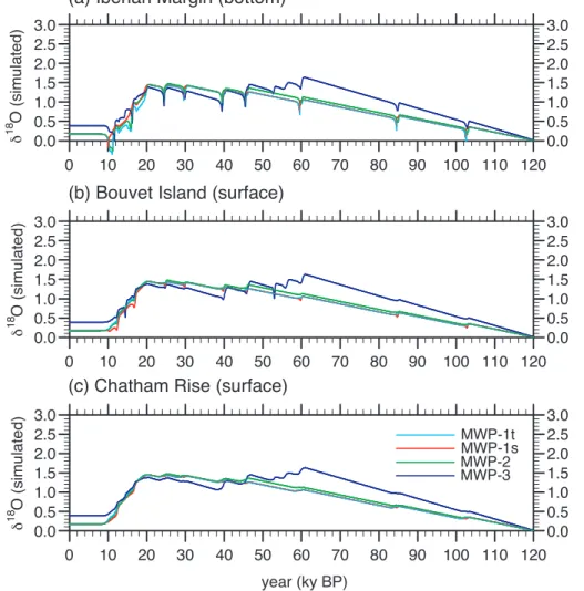
Modelling ocean circulation, climate and oxygen isotopes in the ocean over the last 120 000 years
Texte intégral
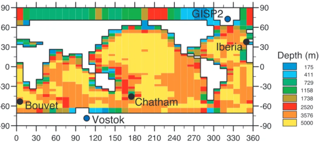
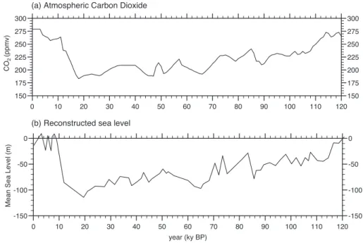
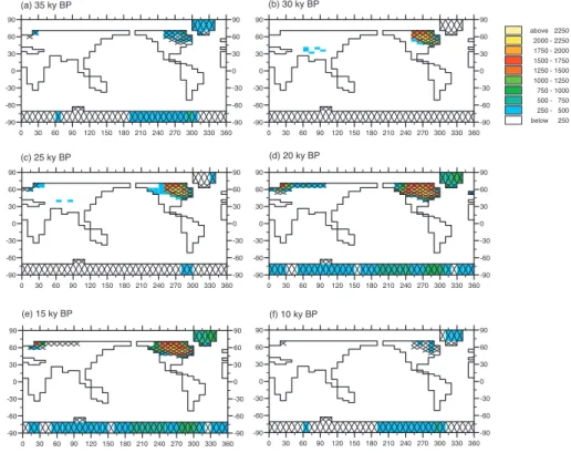
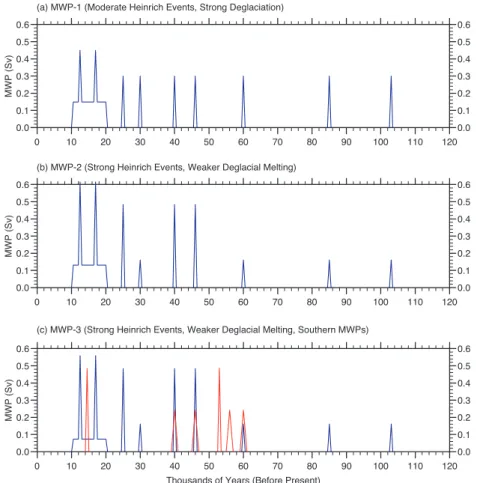
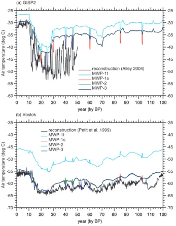
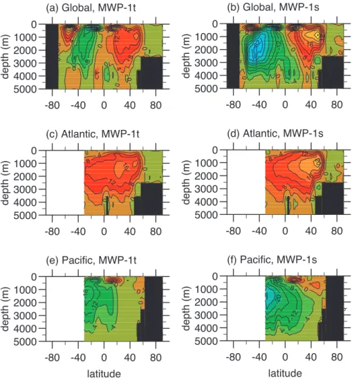
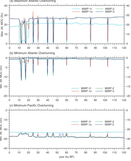
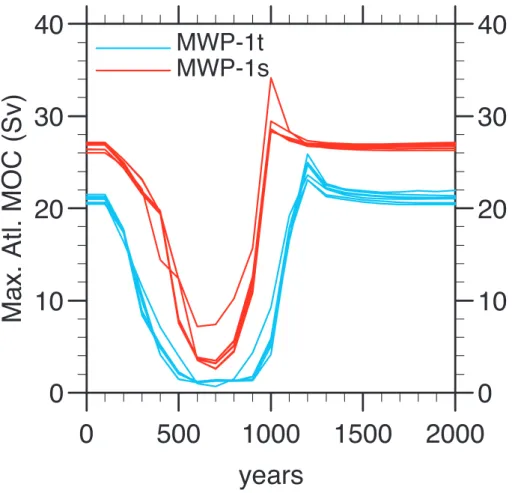
Figure

Documents relatifs
L’accès à ce site Web et l’utilisation de son contenu sont assujettis aux conditions présentées dans le site LISEZ CES CONDITIONS ATTENTIVEMENT AVANT D’UTILISER CE SITE WEB.
The proposed method is a 3 steps procedure: step 1, is an estimation of human risk according to location, vulnerability and building number of occupants – to
Defining algorithmic skeletons with template metaprogramming makes possible the implementation of compile-time algorithms to optimize the distribution of parallel tasks. All this
and is associated with wider UP deformation (see high strain-rate regions in Figure 5.b and Appendix B)... Figure 5: a) Upper plate and trench retreat velocities for
Après onversion et requanti ation du signal sur 9 bits (destiné au al ul de la puissan e de sortie) puis requanti ation sur 2 bits redirigé vers le orrélateur (Figure 1.20), la
Les r´ esultats montrent que les limitations de l’assimilation sont dues aux biais du mod` ele qui persistent encore : difficult´ e pour phaser l’onde de mar´ ee thermique qui
Nous appelerons modèle orthographique la distribution de probabilité (à sup- port infini sur l’ensemble des chaînes de caractères) servant de distribution de base pour la
