Mathematical Analysis I by Zorich pdf - Web Education

(1)

(2)

(3)

Springer

Berlin Heidelberg New York Hong Kong London Milan Paris Tokyo

(4)

Vladimir A. Zorich

Mathematical

Analysis I

(5)

Vladimir A. Zorich

Moscow State University

Department of Mathematics (Mech-Math) Vorobievy Gory 119992 Moscow Russia Translator: Roger Cooke Burlington, Vermont USA e-mail: cooke@emba.uvm.edu

Title of Russian edition:

Matematicheskij Analiz (Part 1,4th corrected edition, Moscow, 2002) MCCME (Moscow Center for Continuous Mathematical Education Publ.)

Cataloging-in-Publication Data applied for

A catalog record for this book is available from the Library of Congress. Bibliographic information published by Die Deutsche Bibliothek

Die Deutsche Bibliothek lists this publication in the Deutsche Nationalbibliografie; detailed bibliographic data is available in the Internet at http://dnb.ddb.de

Mathematics Subject Classification (2000): Primary 00A05 Secondary: 26-01,40-01,42-01,54-01,58-01

ISBN 3-540-40386-8 Springer-Verlag Berlin Heidelberg New York This work is subject to copyright. All rights are reserved, whether the whole or part of the material is concerned, specifically the rights of translation, reprinting, reuse of illustrations, recitation, broadcasting, reproduction on microfilm or in any other way, and storage in data banks. Duplication of this publication or parts thereof is permitted only under the provisions of the German Copyright Law of September 9,1965, in its current version, and permission for use must always be obtained from Springer-Verlag. Violations are liable for prosecution under the German Copyright Law.

Springer-Verlag is a part of Springer Science* Business Media

springeronline.com

© Springer-Verlag Berlin Heidelberg 2004 Printed in Germany

The use of general descriptive names, registered names, trademarks, etc. in this publication does not imply, even in the absence of a specific statement, that such names are exempt from the relevant protective laws and regulations and therefore free for general use.

Cover design: design & production GmbH, Heidelberg Typeset by the translator using a Springer ETgX macro package Printed on acid-free paper 46/3indb- 5 4 3 2

(6)

Prefaces

Preface to the English Edition

An entire generation of mathematicians has grown up during the time be-tween the appearance of the first edition of this textbook and the publication of the fourth edition, a translation of which is before you. The book is famil-iar to many people, who either attended the lectures on which it is based or studied out of it, and who now teach others in universities all over the world. I am glad that it has become accessible to English-speaking readers.

This textbook consists of two parts. It is aimed primarily at university students and teachers specializing in mathematics and natural sciences, and at all those who wish to see both the rigorous mathematical theory and examples of its effective use in the solution of real problems of natural science.

Note that Archimedes, Newton, Leibniz, Euler, Gauss, Poincare, who are held in particularly high esteem by us, mathematicians, were more than mere mathematicians. They were scientists, natural philosophers. In mathematics resolving of important specific questions and development of an abstract gen-eral theory are processes as inseparable as inhaling and exhaling. Upsetting this balance leads to problems that sometimes become significant both in mathematical education and in science in general.

The textbook exposes classical analysis as it is today, as an integral part of the unified Mathematics, in its interrelations with other modern mathe-matical courses such as algebra, differential geometry, differential equations, complex and functional analysis.

Rigor of discussion is combined with the development of the habit of working with real problems from natural sciences. The course exhibits the power of concepts and methods of modern mathematics in exploring spe-cific problems. Various examples and numerous carefully chosen problems, including applied ones, form a considerable part of the textbook. Most of the fundamental mathematical notions and results are introduced and discussed along with information, concerning their history, modern state and creators. In accordance with the orientation toward natural sciences, special attention is paid to informal exploration of the essence and roots of the basic concepts and theorems of calculus, and to the demonstration of numerous, sometimes fundamental, applications of the theory.

(7)

VI Prefaces

For instance, the reader will encounter here the Galilean and Lorentz transforms, the formula for rocket motion and the work of nuclear reac-tor, Euler's theorem on homogeneous functions and the dimensional analysis of physical quantities, the Legendre transform and Hamiltonian equations of classical mechanics, elements of hydrodynamics and the Carnot's theo-rem from thermodynamics, Maxwell's equations, the Dirac delta-function, distributions and the fundamental solutions, convolution and mathematical models of linear devices, Fourier series and the formula for discrete coding of a continuous signal, the Fourier transform and the Heisenberg uncertainty principle, differential forms, de Rham cohomology and potential fields, the theory of extrema and the optimization of a specific technological process, numerical methods and processing the data of a biological experiment, the asymptotics of the important special functions, and many other subjects.

Within each major topic the exposition is, as a rule, inductive, sometimes proceeding from the statement of a problem and suggestive heuristic consider-ations concerning its solution, toward fundamental concepts and formalisms. Detailed at first, the exposition becomes more and more compressed as the course progresses. Beginning ab ovo the book leads to the most up-to-date state of the subject.

Note also that, at the end of each of the volumes, one can find the list of the main theoretical topics together with the corresponding simple, but nonstandard problems (taken from the midterm exams), which are intended to enable the reader both determine his or her degree of mastery of the material and to apply it creatively in concrete situations.

More complete information on the book and some recommendations for its use in teaching can be found below in the prefaces to the first and second Russian editions.

(8)

Prefaces VII

Preface to the Fourth Russian Edition

The time elapsed since the publication of the third edition has been too short for me to receive very many new comments from readers. Nevertheless, some errors have been corrected and some local alterations of the text have been made in the fourth edition.

Moscow, 2002 V. Zorich

Preface to the Third Russian edition

This first part of the book is being published after the more advanced Part 2 of the course, which was issued earlier by the same publishing house. For the sake of consistency and continuity, the format of the text follows that adopted in Part 2. The figures have been redrawn. All the misprints that were noticed have been corrected, several exercises have been added, and the list of further readings has been enlarged. More complete information on the subject matter of the book and certain characteristics of the course as a whole are given below in the preface to the first edition.

Moscow, 2001 V. Zorich

Preface to the Second Russian Edition

In this second edition of the book, along with an attempt to remove the mis-prints that occurred in the first edition,1 certain alterations in the exposition

have been made (mainly in connection with the proofs of individual theo-rems), and some new problems have been added, of an informal nature as a rule.

The preface to the first edition of this course of analysis (see below) con-tains a general description of the course. The basic principles and the aim of the exposition are also indicated there. Here I would like to make a few remarks of a practical nature connected with the use of this book in the classroom.

Usually both the student and the teacher make use of a text, each for his own purposes.

At the beginning, both of them want most of all a book that contains, along with the necessary theory, as wide a variety of substantial examples

1 No need to worry: in place of the misprints that were corrected in the plates

of the first edition (which were not preserved), one may be sure that a host of new misprints will appear, which so enliven, as Euler believed, the reading of a mathematical text.

(9)

VIII Prefaces

of its applications as possible, and, in addition, explanations, historical and scientific commentary, and descriptions of interconnections and perspectives for further development. But when preparing for an examination, the student mainly hopes to see the material that will be on the examination. The teacher likewise, when preparing a course, selects only the material that can and must be covered in the time alloted for the course.

In this connection, it should be kept in mind that the text of the present book is noticeably more extensive than the lectures on which it is based. What caused this difference? First of all, the lectures have been supplemented by essentially an entire problem book, made up not so much of exercises as sub-stantive problems of science or mathematics proper having a connection with the corresponding parts of the theory and in some cases significantly extend-ing them. Second, the book naturally contains a much larger set of examples illustrating the theory in action than one can incorporate in lectures. Third and finally, a number of chapters, sections, or subsections were consciously written as a supplement to the traditional material. This is explained in the sections "On the introduction" and "On the supplementary material" in the preface to the first edition.

I would also like to recall that in the preface to the first edition I tried to warn both the student and the beginning teacher against an excessively long study of the introductory formal chapters. Such a study would noticeably delay the analysis proper and cause a great shift in emphasis.

To show what in fact can be retained of these formal introductory chap-ters in a realistic lecture course, and to explain in condensed form the syllabus for such a course as a whole while pointing out possible variants depending on the student audience, at the end of the book I give a list of problems from the midterm exam, along with some recent examination topics for the first two semesters, to which this first part of the book relates. From this list the professional will of course discern the order of exposition, the degree of development of the basic concepts and methods, and the occasional invoca-tion of material from the second part of the textbook when the topic under consideration is already accessible for the audience in a more general form.2

In conclusion I would like to thank colleagues and students, both known and unknown to me, for reviews and constructive remarks on the first edition of the course. It was particularly interesting for me to read the reviews of A. N. Kolmogorov and V. I. Arnol'd. Very different in size, form, and style, these two have, on the professional level, so many inspiring things in common. Moscow, 1997 V. Zorich

2 Some of the transcripts of the corresponding lectures have been published and I

give formal reference to the booklets published using them, although I understand that they are now available only with difficulty. (The lectures were given and published for limited circulation in the Mathematical College of the Independent University of Moscow and in the Department of Mechanics and Mathematics of Moscow State University.)

(10)

Prefaces IX

Prom the Preface to the First Russian Edition

The creation of the foundations of the differential and integral calculus by Newton and Leibniz three centuries ago appears even by modern standards to be one of the greatest events in the history of science in general and mathematics in particular.

Mathematical analysis (in the broad sense of the word) and algebra have intertwined to form the root system on which the ramified tree of modern mathematics is supported and through which it makes its vital contact with the nonmathematical sphere. It is for this reason that the foundations of analysis are included as a necessary element of even modest descriptions of so-called higher mathematics; and it is probably for that reason that so many books aimed at different groups of readers are devoted to the exposition of the fundamentals of analysis.

This book has been aimed primarily at mathematicians desiring (as is proper) to obtain thorough proofs of the fundamental theorems, but who are at the same time interested in the life of these theorems outside of mathe-matics itself.

The characteristics of the present course connected with these circum-stances reduce basically to the following:

In the exposition. Within each major topic the exposition is as a rule

induc-tive, sometimes proceeding from the statement of a problem and suggestive heuristic considerations toward its solution to fundamental concepts and for-malisms.

Detailed at first, the exposition becomes more and more compressed as the course progresses.

An emphasis is placed on the efficient machinery of smooth analysis. In the exposition of the theory I have tried (to the extent of my knowledge) to point out the most essential methods and facts and avoid the temptation of a minor strengthening of a theorem at the price of a major complication of its proof.

The exposition is geometric throughout wherever this seemed worthwhile in order to reveal the essence of the matter.

The main text is supplemented with a rather large collection of examples, and nearly every section ends with a set of problems that I hope will sig-nificantly complement even the theoretical part of the main text. Following the wonderful precedent of Polya and Szego, I have often tried to present a beautiful mathematical result or an important application as a series of problems accessible to the reader.

The arrangement of the material was dictated not only by the architecture of mathematics in the sense of Bourbaki, but also by the position of analysis as a component of a unified mathematical or, one should rather say, natural-science/mathematical education.

(11)

X Prefaces

The present Part 1 contains the differential and integral calculus of func-tions of one variable and the differential calculus of funcfunc-tions of several vari-ables.

In differential calculus we emphasize the role of the differential as a linear standard for describing the local behavior of the variation of a variable. In ad-dition to numerous examples of the use of differential calculus to study func-tional relations (monotonicity, extrema) we exhibit the role of the language of analysis in writing simple differential equations - mathematical models of real-world phenomena and the substantive problems connected with them.

We study a number of such problems (for example, the motion of a body of variable mass, a nuclear reactor, atmospheric pressure, motion in a resisting medium) whose solution leads to important elementary functions. Full use is made of the language of complex variables; in particular, Euler's formula is derived and the unity of the fundamental elementary functions is shown.

The integral calculus has consciously been explained as far as possible using intuitive material in the framework of the Riemann integral. For the majority of applications, this is completely adequate.3 Various applications

of the integral are pointed out, including those that lead to an improper in-tegral (for example, the work involved in escaping from a gravitational field, and the escape velocity for the Earth's gravitational field) or to elliptic func-tions (motion in a gravitational field in the presence of constraints, pendulum motion.)

The differential calculus of functions of several variables is very geometric. In this topic, for example, one studies such important and useful consequences of the implicit function theorem as curvilinear coordinates and local reduction to canonical form for smooth mappings (the rank theorem) and functions (Morse's lemma), and also the theory of extrema with constraint.

Results from the theory of continuous functions and differential calculus are summarized and explained in a general invariant form in two chapters that link up naturally with the differential calculus of real-valued functions of several variables. These two chapters open the second part of the course. The second book, in which we also discuss the integral calculus of functions of several variables up to the general Newton-Leibniz-Stokes formula thus acquires a certain unity.

We shall give more complete information on the second book in its preface. At this point we add only that, in addition to the material already mentioned, it contains information on series of functions (power series and Fourier series included), on integrals depending on a parameter (including the fundamental solution, convolution, and the Fourier transform), and also on asymptotic expansions (which are usually absent or insufficiently presented in textbooks).

We now discuss a few particular problems.

3 The "stronger" integrals, as is well known, require fussier set-theoretic

consider-ations, outside the mainstream of the textbook, while adding hardly anything to the effective machinery of analysis, mastery of which should be the first priority.

(12)

Prefaces XI

On the introduction. I have not written an introductory survey of the subject,

since the majority of beginning students already have a preliminary idea of differential and integral calculus and their applications from high school, and I could hardly claim to write an even more introductory survey. Instead, in the first two chapters I bring the former high-school student's understanding of sets, functions, the use of logical symbolism, and the theory of a real number to a certain mathematical completeness.

This material belongs to the formal foundations of analysis and is aimed primarily at the mathematics major, who may at some time wish to trace the logical structure of the basic concepts and principles used in classical analysis. Mathematical analysis proper begins in the third chapter, so that the reader who wishes to get effective machinery in his hands as quickly as possible and see its applications can in general begin a first reading with Chapter 3, turning to the earlier pages whenever something seems nonobvious or raises a question which hopefully I also have thought of and answered in the early chapters.

On the division of material The material of the two books is divided into

chapters numbered continuously. The sections are numbered within each chapter separately; subsections of a section are numbered only within that section. Theorems, propositions, lemmas, definitions, and examples are writ-ten in italics for greater logical clarity, and numbered for convenience within each section.

On the supplementary material. Several chapters of the book are written as a

natural extension of classical analysis. These are, on the one hand, Chapters 1 and 2 mentioned above, which are devoted to its formal mathematical foundations, and on the other hand, Chapters 9, 10, and 15 of the second part, which give the modern view of the theory of continuity, differential and integral calculus, and finally Chapter 19, which is devoted to certain effective asymptotic methods of analysis.

The question as to which part of the material of these chapters should be included in a lecture course depends on the audience and can be decided by the lecturer, but certain fundamental concepts introduced here are usually present in any exposition of the subject to mathematicians.

In conclusion, I would like to thank those whose friendly and competent professional aid has been valuable and useful to me during the work on this book.

The proposed course was quite detailed, and in many of its aspects it was coordinated with subsequent modern university mathematics courses -such as, for example, differential equations, differential geometry, the theory of functions of a complex variable, and functional analysis. In this regard my contacts and discussions with V. I. Arnol'd and the especially numerous ones with S. P. Novikov during our joint work with the so-called "experimental student group in natural-science/mathematical education" in the Department of Mathematics at MSU, were very useful to me.

(13)

XII Prefaces

I received much advice from N. V. Efimov, chair of the Section of Math-ematical Analysis in the Department of Mechanics and Mathematics at Moscow State University.

I am also grateful to colleagues in the department and the section for remarks on the mimeographed edition of my lectures.

Student transcripts of my recent lectures which were made available to me were valuable during the work on this book, and I am grateful to their owners.

I am deeply grateful to the official reviewers L. D. Kudryavtsev, V. P. Pet-renko, and S.B.Stechkin for constructive comments, most of which were taken into account in the book now offered to the reader.

(14)

1 Some General Mathematical Concepts

and Notation

1.1 Logical Symbolism

1.1.1 C o n n e c t i v e s a n d B r a c k e t s

T h e language of this book, like t h e majority of m a t h e m a t i c a l t e x t s , consists of ordinary language and a number of special symbols from t h e theories being discussed. Along with t h e special symbols, which will be introduced as needed, we use t h e common symbols of m a t h e m a t i c a l logic -i, A, V, =>, and <^> to denote respectively negation (not) a n d t h e logical connectives and,

or, implies, a n d is equivalent to.1

For example, take three s t a t e m e n t s of independent interest:

L. If the notation is adapted to the discoveries..., the work of thought is

marvelously shortened. (G. Leibniz)2

P. Mathematics is the art of calling different things by the same name.

( H . P o i n c a r e ) .3

G. The great book of nature is written in the language of mathematics.

(Galileo).4

T h e n , according to t h e notation given above,

1 The symbol & is often used in logic in place of A. Logicians more often write

the implication symbol => as —> and the relation of logical equivalence as <—> or o . However, we shall adhere to the symbolism indicated in the text so as not to overburden the symbol ->, which has been traditionally used in mathematics to denote passage to the limit.

2 G.W.Leibniz (1646-1716) - outstanding German scholar, philosopher, and

mathematician to whom belongs the honor, along with Newton, of having dis-covered the foundations of the infinitesimal calculus.

3 H.Poincare (1854-1912) - French mathematician whose brilliant mind

trans-formed many areas of mathematics and achieved fundamental applications of it in mathematical physics.

4 Galileo Galilei (1564-1642) - Italian scholar and outstanding scientific

experi-menter. His works lie at the foundation of the subsequent physical concepts of space and time. He is the father of modern physical science.

(21)

2 1 Some General Mathematical Concepts and Notation

Notation Meaning

L=> P L implies P L <3> P L is equivalent to P

((L => P)A (-iP)) => (-.L) If P follows from L and P is false, then L is false

-i((L <£> G) V ( P <£> G)) G is not equivalent either to L or to P We see that it is not always reasonable to use only formal notation, avoid-ing colloquial language.

We remark further that parentheses are used in the writing of complex statements composed of simpler ones, fulfilling the same syntactical function as in algebraic expressions. As in algebra, in order to avoid the overuse of parentheses one can make a convention about the order of operations. To that end, we shall agree on the following order of priorities for the symbols:

- i , A , V , = * , < * .

With this convention the expression -^AABVC => D should be interpreted

as (((-"-A) A B) V C) => D, and the relation A V B => C as (A V B) => C, not as AV(B=>C).

We shall often give a different verbal expression to the notation A => JB, which means that A implies B, or, what is the same, that B follows from A, saying that B is a necessary criterion or necessary condition for A and A in turn is a sufficient condition or sufficient criterion for B, so that the relation

A O B can be read in any of the following ways: A is necessary and sufficient for B\

A hold when B holds, and only then; A if and only if B\

A is equivalent to B.

Thus the notation A O B means that A implies B and simultaneously B implies A.

The use of the conjunction and in the expression A A B requires no ex-planation.

It should be pointed out, however, that in the expression A V B the con-junction or is not exclusive, that is, the statement A V B is regarded as true if at least one of the statements A and B is true. For example, let x be a real number such that x2 — 3x + 2 = 0. Then we can write that the following

relation holds:

(x2 - 3x + 2 = 0) & (x = 1) V (x = 2) .

1.1.2 Remarks on Proofs

A typical mathematical proposition has the form A => JB, where A is the assumption and B the conclusion. The proof of such a proposition consists of

(22)

1.1 Logical Symbolism 3 constructing a chain A => C\ => • • • => Cn => B of implications, each element

of which is either an axiom or a previously proved proposition.5

In proofs we shall adhere to the classical rule of inference: if A is true and

A => JB, then B is also true.

In proof by contradiction we shall also use the law of excluded middle, by virtue of which the statement A V -*A (A or not-^4) is considered true independently of the specific content of the statement A. Consequently we simultaneously accept that ~*(-*A) <£> A, that is, double negation is equivalent to the original statement.

1.1.3 Some Special Notation

For the reader's convenience and to shorten the writing, we shall agree to denote the end of a proof by the symbol • .

We also agree, whenever convenient, to introduce definitions using the special symbol := (equality by definition), in which the colon is placed on the side of the object being defined.

For example, the notation b

f(x)dx:= hm a ( / ; P , 0 J A(P)-X)

a

defines the left-hand side in terms of the right-hand side, whose meaning is assumed to be known.

Similarly, one can introduce abbreviations for expressions already defined. For example

n

2 = 1

introduces the notation a(f; P, £) for the sum of special form on the left-hand side.

1.1.4 Concluding Remarks

We note that here we have spoken essentially about notation only, without analyzing the formalism of logical deductions and without touching on the profound questions of truth, provability, and deducibility, which form the subject matter of mathematical logic.

How are we to construct mathematical analysis if we have no formalization of logic? There may be some consolation in the fact that we always know more than we can formalize at any given time, or perhaps we should say we know how to do more than we can formalize. This last sentence may be clarified by

(23)

the well-known proverb of the centipede who forgot how to walk when asked to explain exactly how it dealt with so many legs.

The experience of all the sciences convinces us that what was consid-ered clear or simple and unanalyzable yesterday may be subjected to re-examination or made more precise today. Such was the case (and will un-doubtedly be the case again) with many concepts of mathematical analysis, the most important theorems and machinery of which were discovered in the seventeenth and eighteenth centuries, but which acquired its modern formal-ized form with a unique interpretation that is probably responsible for its being generally accessible, only after the creation of the theory of limits and the fully developed theory of real numbers needed for it in the nineteenth century.

This is the level of the theory of real numbers from which we shall begin to construct the whole edifice of analysis in Chap. 2.

As already noted in the preface, those who wish to make a rapid ac-quaintance with the basic concepts and effective machinery of differential and integral calculus proper may begin immediately with Chap. 3, turning to particular places in the first two chapters only as needed.

1.1.5 Exercises

We shall denote true assertions by the symbol 1 and false ones by 0. Then to each of the statements -u4, A A J3, A V J3, and A => B one can associate a so-called

truth table, which indicates its truth or falsehood depending on the truth of the

statements A and B. These tables are a formal definition of the logical operations -i, A, V, =». Here they are:

AVB A ^A 0 1 1 0 0 1 0 0 1 1 1 1 AAB B \B 0 1 0 0 0 1 0 1 0 1 0 1 0 1 1 1

1. Check whether all of these tables agree with your concept of the corresponding logical operation. (In particular, pay attention to the fact that if A is false, then the implication A =» B is always true.)

(24)

1.2 Sets and Elementary Operations on them 5 2. Show that the following simple, but very useful relations, which are widely used in mathematical reasoning, are true:

a) -.(A A B) <& ^A V -.J5; b) -.(AVJ5) <^--AA-.J5; c) (A => J5) <^ (-.J5 => --A); d) (A=^J5)<^(-AVJ5); e) -.(A => J5) ^ A A -.J5.

1.2 Sets and Elementary Operations on them

1.2.1 The Concept of a Set

Since the late nineteenth and early twentieth centuries the most universal language of mathematics has been the language of set theory. This is even manifest in one of the definitions of mathematics as the science that studies different structures (relations) on sets.6

"We take a set to be an assemblage of definite, perfectly distinguishable objects of our intuition or our thought into a coherent whole." Thus did Georg Cantor,7 the creator of set theory, describe the concept of a set.

Cantor's description cannot, of course, be considered a definition, since it appeals to concepts that may be more complicated than the concept of a set itself (and in any case, have not been defined previously). The purpose of this description is to explain the concept by connecting it with other concepts.

The basic assumptions of Cantorian (or, as it is generally called, "naive") set theory reduce to the following statements.

1°. A set may consist of any distinguishable objects.

2°. A set is unambiguously determined by the collection of objects that com-prise it.

3°. Any property defines the set of objects having that property.

If x is an object, P is a property, and P(x) denotes the assertion that x has property P , then the class of objects having the property P is denoted

{x\ P(x)}. The objects that constitute a class or set are called the elements

of the class or set.

The set consisting of the elements X\,..., xn is usually denoted

{xi,... , xn} . Wherever no confusion can arise we allow ourselves to denote

the one-element set {a} simply as a.

6 Bourbaki, N. "The architecture of mathematics" in: N. Bourbaki, Elements of the history of mathematics, translated from the French by John Meldrum, Springer,

New York, 1994.

7 G. Cantor (1845-1918) - German mathematician, the creator of the theory of

(25)

The words "class", "family", "totality", and "collection" are used as syn-onyms for "set" in naive set theory.

The following examples illustrate the application of this terminology: — the set of letters "a" occurring in the word "I";

— the set of wives of Adam;

— the collection of ten decimal digits; — the family of beans;

— the set of grains of sand on the Earth;

— the totality of points of a plane equidistant from two given points of the plane;

— the family of sets; — the set of all sets.

The variety in the possible degree of determinacy in the definition of a set leads one to think that a set is, after all, not such a simple and harmless concept.

And in fact the concept of the set of all sets, for example, is simply contradictory.

Proof. Indeed, suppose that for a set M the notation P(M) means that M

is not an element of itself.

Consider the class K = {M\ P(M)} of sets having property P.

If K is a set either P(K) or -*P(K) is true. However, this dichotomy does not apply to K. Indeed, P{K) is impossible; for it would then follow from the definition of K that K contains K as an element, that is, that -*P(K) is true; on the other hand, -*P(K) is also impossible, since that means that K contains K as an element, which contradicts the definition of K as the class of sets that do not contain themselves as elements.

Consequently K is not a set. •

This is the classical paradox of Russell,8 one of the paradoxes to which

the naive conception of a set leads.

In modern mathematical logic the concept of a set has been subjected to detailed analysis (with good reason, as we see). However, we shall not go into that analysis. We note only that in the current axiomatic set theories a set is defined as a mathematical object having a definite collection of properties. The description of these properties constitutes an axiom system. The core of axiomatic set theory is the postulation of rules by which new sets can be formed from given ones. In general any of the current axiom systems is such that, on the one hand, it eliminates the known contradictions of the naive theory, and on the other hand it provides freedom to operate with specific sets that arise in different areas of mathematics, most of all, in mathematical analysis understood in the broad sense of the word.

8 B.Russell (1872-1970) - British logician, philosopher, sociologist and social

(26)

1.2 Sets and Elementary Operations on them 7 Having confined ourselves for the time being to remarks on the concept of a set, we pass to the description of the set-theoretic relations and operations most commonly used in analysis.

Those wishing a more detailed acquaintance with the concept of a set should study Subsect. 1.4.2 in the present chapter or turn to the specialized literature.

1.2.2 The Inclusion Relation

As has already been pointed out, the objects that comprise a set are usually called the elements of the set. We tend to denote sets by uppercase letters and their elements by the corresponding lowercase letters.

The statement, "x is an element of the set X" is written briefly as

x eX (or X 3 x) ,

and its negation as

x $ X ( o r l ^ x ) .

When statements about sets are written, frequent use is made of the logical operators 3 ("there exists" or "there are") and V ("every" or "for any") which are called the existence and generalization quantifiers respectively.

For example, the string Vx((x G A) <$> (x G B)) means that for any object

x the relations x G A and x G B are equivalent. Since a set is completely

determined by its elements, this statement is usually written briefly as

A = B,

read "A equals JB" , and means that the sets A and B are the same. Thus two sets are equal if they consist of the same elements. The negation of equality is usually written as A ^ B.

If every element of A is an element of B, we write A c B or B D A and say that A is a subset of B or that B contains A or that B includes A. In this connection the relation A C B between sets A and B is called the inclusion

relation (Fig. 1.1).

Fig. 1.1. M

(27)

8 1 Some General Mathematical Concepts and Notation Thus

(A C B) := Vx((x eA)=>(xe B)) .

If A C B and A ^ JB, we shall say that the inclusion A C B is s£ric£ or that ^4 is a proper subset of B.

Using these definitions, we can now conclude that

(A = B)<*(AcB)A(BcA).

If M is a set, any property P distinguishes in M the subset

{xeM\P{x)}

consisting of the elements of M that have the property. For example, it is obvious that

M = {x e M\x e M} .

On the other hand, if P is taken as a property that no element of the set M has, for example, P(x) := (a: / x), we obtain the set

0 = {x e M\x ^ x} , called the empty subset of M.

1.2.3 Elementary Operations on Sets

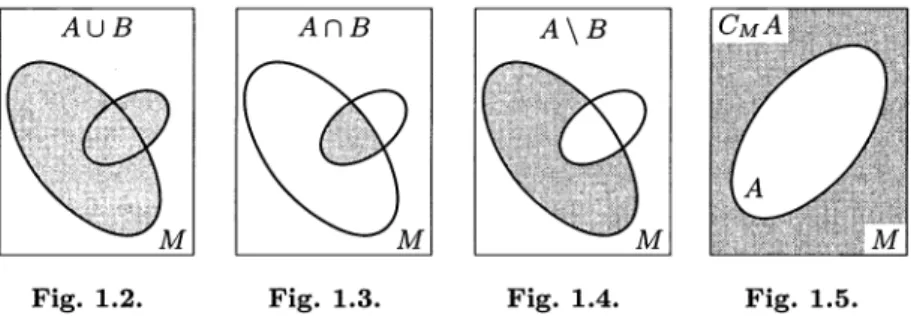
Let A and B be subsets of a set M. a. The union of A and B is the set

AU B := {x e M\(x e A) V (x e B)} ,

consisting of precisely the elements of M that belong to at least one of the sets A and B (Fig. 1.2).

b . The intersection of A and B is the set

Af)B := {xeM\(x eA) A(xe B)} ,

formed by the elements of M that belong to both sets A and B (Fig. 1.3). c. The difference between A and B is the set

A\B:={xe M\ {xeA)A(x£ B)} ,

consisting of the elements of A that do not belong to B (Fig. 1.4).

The difference between the set M and one of its subsets A is usually called the complement of A in M and denoted CM A, or CA when the set in which the complement of A is being taken is clear from the context (Fig. 1.5).

(28)

1.2 Sets and Elementary Operations on them 9

Fig. 1.2. Fig. 1.3. Fig. 1.4. Fig. 1.5.

Example. As an illustration of the interaction of the concepts just

intro-duced, let us verify the following relations (the so-called de Morgan9 rules):

CM(AUB) = CMAnCMB , (1.1)

CM(A H B) = CMA U CMB . (1.2)

Proof. We shall prove the first of these equalities by way of example: (x e CM(A U B)) => (x i (A U B)) => ((x £A)A(x(£ B)) =>

=> (x e CMA) A(xe CMB) => (x e (CMA n CMB)) .

Thus we have established that

CM(A UB)C (CMA n CMB) . (1.3)

On the other hand,

(x e (CMA n CMB)) => ((x e CMA) A(xe CMB)) =>

=> ((x iA)A(x£ B)) =>(x£(A[J B)) =>

=» (xeCM(AUB)) ,

that is,

(CMA n CMB) C CM(A U B) . (1.4)

Equation (1.1) follows from (1.3) and (1.4). •

d. The direct (Cartesian) product of sets. For any two sets A and B one can form a new set, namely the pair {A,B} = {B,A}, which consists of the sets

A and B and no others. This set has two elements if A ^ B and one element iiA = B.

This set is called the unordered pair of sets A and JB, to be distinguished from the ordered pair (A,B) in which the elements are endowed with ad-ditional properties to distinguish the first and second elements of the pair

(29)

{A,B}. The equality

(A,B) = (C,D)

between two ordered pairs means by definition that A = C and B = D. In particular, if A ^ B, then (A, B) ^ (B, A).

Now let X and Y be arbitrary sets. The set

XxY:={(x,y)\(x€X)A(y£Y)},

formed by the ordered pairs (x, y) whose first element belongs to X and whose second element belongs to Y, is called the direct or Cartesian product of the sets X and Y (in that order!).

It follows obviously from the definition of the direct product and the remarks made above about the ordered pair that in general X xY ^Y x X. Equality holds only if X = Y. In this last case we abbreviate X x X as X2.

The direct product is also called the Cartesian product in honor of Descartes,10 who arrived at the language of analytic geometry in terms of

a system of coordinates independently of Fermat.11 The familiar system of

Cartesian coordinates in the plane makes this plane precisely into the direct product of two real axes. This familiar object shows vividly why the Cartesian product depends on the order of the factors. For example, different points of the plane correspond to the pairs (0,1) and (1,0).

In the ordered pair z = (xi, x2), which is an element of the direct product

Z = Xi x X2 of the sets X\ and X2, the element x\ is called the first projection

of the pair z and denoted p r ^ , while the element x2 is the second projection

of z and is denoted pr2z.

By analogy with the terminology of analytic geometry, the projections of an ordered pair are often called the (first and second) coordinates of the pair. 1.2.4 Exercises

In Exercises 1,2, and 3 the letters A, B, and C denote subsets of a set M. 1. Verify the following relations.

a) (AcC)A(BcC)<> ((A U 5 ) c c ) ; b) (CcA)A(CcB)o ( c c ( A n B ) ) ;

c)CM(cMA) = A;

d) (A C CMB) o(Bc CM A)-,

e) (AcB)o {CMA D CMB).

10 R.Descartes (1596-1650) - outstanding French philosopher, mathematician and

physicist who made fundamental contributions to scientific thought and knowl-edge.

11 P. Fermat (1601-1665) - remarkable French mathematician, a lawyer by

profes-sion. He was one of the founders of a number of areas of modern mathematics: analysis, analytic geometry, probability theory, and number theory.

(30)

1.3 Functions 11 2. Prove the following statements.

a) A U (B.U C) = (AuB)uC=:AuBuC;

b) AH (B DC) = (An B) PiC =: AH B DC;

c) A n ( £ U C) = (A n £ ) U (A n C);

d)Au(5nC) = (Au5)n(Au C).

3. Verify the connection (duality) between the operations of union and intersection: a) CM(A U B) = CMA n CM# ;

b) CM (A nB) = CM A U CMB.

4. Give geometric representations of the following Cartesian products. a) The product of two line segments (a rectangle).

b) The product of two lines (a plane).

c) The product of a line and a circle (an infinite cylindrical surface). d) The product of a line and a disk (an infinite solid cylinder). e) The product of two circles (a torus).

f) The product of a circle and a disk (a solid torus).

5. The set A = { ( r c i , ^ ) G X2\xi = X2} is called the diagonal of the Cartesian square X2 of the set X. Give geometric representations of the diagonals of the sets obtained in parts a), b), and e) of Exercise 4.

6. Show that

a) (X xY = 0) O (X = 0)V (Y = 0 ) , and if X x Y ^ 0 , then b) (AxBcX xY)o(AcX)A(BcY),

c) (X x Y) U (Z x Y) = (X U Z) x y ,

d) ( i x y ) n (x' x Y') = (xn x') x (y n Y').

Here 0 denotes the empty set, that is, the set having no elements.

7. By comparing the relations of Exercise 3 with relations a) and b) from Exercise 2 of Sect. 1.1, establish a correspondence between the logical operators -1, A, V and the operations C, n, and U on sets.

1.3 Functions

1.3.1 T h e C o n c e p t o f a F u n c t i o n ( M a p p i n g )

We shall now describe t h e concept of a functional relation, which is funda-mental b o t h in m a t h e m a t i c s and elsewhere.

Let X and Y be certain sets. We say t h a t t h e r e is a function defined on

X with values in Y if, by virtue of some rule / , t o each element x € X t h e r e

corresponds an element y G Y.

In this case t h e set X is called t h e domain of definition of t h e function. T h e symbol x used t o denote a general element of t h e domain is called t h e

(31)

argument of the function, or the independent variable. The element yo G Y

corresponding to a particular value xo G X of the argument x is called the

value of the function at x$, or the value of the function at the value x = xo

of its argument, and is denoted f(xo). As the argument x G X varies, the value y = f(x) G Y, in general, varies depending on the values of x. For that reason, the quantity y = f(x) is often called the dependent variable.

The set

f(X) := {y e Y\ 3x ((* € X) A (y = f(x)))}

of values assumed by a function on elements of the set X will be called the

set of values or the range of the function.

The term "function" has a variety of useful synonyms in different areas of mathematics, depending on the nature of the sets X and Y: mapping,

transformation, morphism, operator, functional. The commonest is mapping,

and we shall also use it frequently.

For a function (mapping) the following notations are standard:

/ : X -» y, X -A Y .

When it is clear from the context what the domain and range of a function are, one also uses the notation x i-* f(x) or y = f(x), but more frequently a function in general is simply denoted by the single symbol / .

Two functions f\ and f^ are considered identical or equal if they have the same domain X and at each element x G X the values f\(x) and f2(x) are the same. In this case we write f\ =

fi-If A C X and / : X -» Y is a function, we denote by f\A or f\^ the function (p : A —» Y that agrees with / on A. More precisely, / | A ( # ) := <p(x)

if x G A. The function / | ^ is called the restriction of / to A, and the function / : X —» Y is called an extension or a continuation of (p to X.

We see that it is sometimes necessary to consider a function (p : A —» F defined on a subset A of some set X while the range <p(A) of <p may also turn out be a subset of Y that is different from Y. In this connection, we sometimes use the term domain of departure of the function to denote any set X containing the domain of a function, and domain of arrival to denote any subset of Y containing its range.

Thus, defining a function (mapping) involves specifying a triple (X, Y, / ) , where

X is the set being mapped, or domain of the function;

Y is the set into which the mapping goes, or a domain of arrival of the

function;

/ is the rule according to which a definite element y G Y is assigned to each element x G X.

The asymmetry between X and Y that appears here reflects the fact that the mapping goes from X to F , and not the other direction.

(32)

1.3 Functions 13

Example 1. The formulas / = 2nr and V = f^n*3 establish functional rela-tionships between the circumference / of a circle and its radius r and between the volume V of a ball and its radius r. Each of these formulas provides a particular function / : R+ —» R+ defined on the set R+ of positive real

numbers with values in the same set.

Example 2. Let X be the set of inertial coordinate systems and c : X —» R

the function that assigns to each coordinate system x € X the value c(x) of the speed of light in vacuo measured using those coordinates. The function

c : X —» R is constant, that is, for any x G X it has the same value c. (This

is a fundamental experimental fact.)

Example 3. The mapping G : R2 -> R2 (the direct product R2 = R x R =

Rt x Rx of the time axis R$ and the spatial axis Rx) into itself defined by the

formulas

x' = x — vt , t' = t ,

is the classical Galilean transformation for transition from one inertial coor-dinate system (x,i) to another system (xf,tf) that is in motion relative to

the first at speed v.

The same purpose is served by the mapping L : R2 -> R2 defined by the

relations

, _ x — vt

This is the well-known (one-dimensional) Lorentz12 transformation, which

plays a fundamental role in the special theory of relativity. The speed c is the speed of light.

Example 4- The projection p ^ : X\ x X2 -> X\ defined by the

correspon-dence X\ x X2 3 {x\,X2) "—V x\ G l i is obviously a function. The second projection pr2 : X\ x X2 —> X2 is defined similarly.

Example 5. Let V(M) be the set of subsets of the set M . To each set A G V(M) we assign the set CMA G V(M), that is, the complement to

A in M. We then obtain a mapping CM : ^ ( M ) -> P ( M ) of the set V(M)

into itself.

12 H. A. Lorentz (1853-1928) - Dutch physicist. He discovered these transformations

in 1904, and Einstein made crucial use of them when he formulated his special theory of relativity in 1905.

(33)

Example 6. Let E c M. The real-valued function \E • M -» R defined on

the set M by the conditions (x£?(#) = 1 if a: G JE7) A ( X E ( # ) = 0 if a; G CME) is called the characteristic function of the set i£.

Example 7. Let M ( X ; F ) be the set of mappings of the set X into the set Y and xo a fixed element of X. To any function / G M ( X ; Y) we assign

its value f(xo) G F at the element x$. This relation defines a function F :

M(X; Y) —» y . In particular, if F = R, that is, Y is the set of real numbers,

then to each function / : X —» R the function F : M ( X ; R ) —» R assigns the number F ( / ) = f(xo). Thus F is a function defined on functions. For convenience, such functions are called Junctionals.

Example 8. Let r be the set of curves lying on a surface (for example, the

surface of the earth) and joining two given points of the surface. To each curve 7 G r one can assign its length. We then obtain a function F : r —» R that often needs to be studied in order to find the shortest curve, or as it is called, the geodesic between the two given points on the surface.

Example 9. Consider the set M(R; R) of real-valued functions defined on the

entire real line R. After fixing a number a G R, we assign to each function / G M(R;R) the function Ja G M(R;R) connected with it by the relation

Ja(x) = J(x + a). The function Ja(x) is usually called the translate or shift

of the function / by a. The mapping A : M(R; R) -» M(R; R) that arises in this way is called the translation of shijt operator. Thus the operator A is defined on functions and its values are also functions Ja = A(J).

This last example might seem artificial if not for the fact that we encounter real operators at every turn. Thus, any radio receiver is an operator / i—> J that transforms electromagnetic signals / into acoustic signals / ; any of our sensory organs is an operator (transformer) with its own domain of definition and range of values.

Example 10. The position of a particle in space is determined by an ordered

triple of numbers (x,y,z) called its spatial coordinates. The set of all such ordered triples can be thought of as the direct product R x R x R = R3 of

three real lines R.

A particle in motion is located at some point of the space R3 having

coordinates (x(t),y(t),z(t)) at each instant t of time. Thus the motion of a particle can be interpreted as a mapping 7 : R —» R3, where R is the time

axis and R3 is three-dimensional space.

If a system consists of n particles, its configuration is defined by the position of each of the particles, that is, it is defined by an ordered set (a?i, 2/1, z\\, X21V2, z>2\ • • •; %ni Vn, Zn) consisting of 3n numbers. The set of all such ordered sets is called the configuration space of the system of n parti-cles. Consequently, the configuration space of a system of n particles can be interpreted as the direct product R3 x R3 x • • • x R3 = R3 n of n copies of R3.

To the motion of a system of n particles there corresponds a mapping 7 : R —> R3 n of the time axis into the configuration space of the system.

(34)

1.3 Functions 15

Example 11. The potential energy U of a mechanical system is connected

with the mutual positions of the particles of the system, that is, it is deter-mined by the configuration that the system has. Let Q be the set of possible configurations of a system. This is a certain subset of the configuration space of the system. To each position q G Q there corresponds a certain value U(q) of the potential energy of the system. Thus the potential energy is a function

U : Q —» R defined on a subset Q of the configuration space with values in

the domain R of real numbers.

Example 12. The kinetic energy K of a system of n material particles depends

on their velocities. The total mechanical energy of the system 2£, defined as

E = K + £/, that is, the sum of the kinetic and potential energies, thus

depends on both the configuration q of the system and the set of velocities

v of its particles. Like the configuration q of the particles in space, the set of

velocities v, which consists of n three-dimensional vectors, can be defined as an ordered set of 3n numbers. The ordered pairs (<?, v) corresponding to the states of the system form a subset $ in the direct product R3 n x R3 n = R6 n,

called the phase space of the system of n particles (to be distinguished from the configuration space R3 n) .

The total energy of the system is therefore a function E : $ —» R defined on the subset $ of the phase space R6 n and assuming values in the domain

R of real numbers.

In particular, if the system is closed, that is, no external forces are acting on it, then by the law of conservation of energy, at each point of the set $ of states of the system the function E will have the same value EoGM.

1.3.2 Elementary Classification of Mappings

When a function / : X —» Y is called a mapping, the value f(x) G Y that it assumes at the element x eY is usually called the image of x.

The image of a set A C X under the mapping / : X —» Y is defined as the set

f(A) := {y G Y\ 3x((x &A)A(y = / ( * ) ) ) }

consisting of the elements of Y that are images of elements of A. The set

f-1(B):={xeX\f(x)eB}

consisting of the elements of X whose images belong to B is called the

pre-image (or complete pre-pre-image) of the set B c Y (Fig. 1.6).

A mapping / : X —> Y is said to be

surjective (a mapping of X onto Y) if f(X) = Y;

infective (or an imbedding or injection) if for any elements ^1,^2 of X

( / ( z i ) = /(z2)) => (xi =x2) ,

(35)

Fig. 1.6.

bijective (or a one-to-one correspondence) if it is both surjective and

in-ject ive.

If the mapping / : X —» Y is bijective, that is, it is a one-to-one corre-spondence between the elements of the sets X and F , there naturally arises a mapping

defined as follows: if f(x) = y, then f~1(y) = x, that is, to each element

y G Y one assigns the element x G X whose image under the mapping / is y.

By the surjectivity of / there exists such an element, and by the injectivity of / , it is unique. Hence the mapping f~l is well-defined. This mapping is

called the inverse of the original mapping / .

It is clear from the construction of the inverse mapping that f~l : Y -» X

is itself bijective and that its inverse ( /_ 1)_ 1 : X —» Y is the same as the

original mapping / : X —» Y.

Thus the property of two mappings of being inverses is reciprocal: if f~l

is inverse for / , then / is inverse for /_ 1.

We remark that the symbol f~1(B) for the pre-image of a set B C Y

involves the symbol f~l for the inverse function; but it should be kept in

mind that the pre-image of a set is defined for any mapping / : X -» Y, even if it is not bijective and hence has no inverse.

1.3.3 Composition of Functions and Mutually Inverse Mappings

The operation of composition of functions is on the one hand a rich source of new functions and on the other hand a way of resolving complex functions into simpler ones.

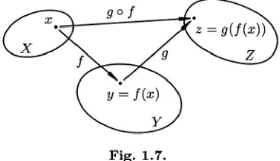
If the mappings / : X -» Y and g : Y -» Z are such that one of them (in our case g) is defined on the range of the other (/), one can construct a new mapping

(36)

1.3 Functions 17 whose values on elements of the set X are defined by the formula

(gof)(x):=g(f(x)).

The compound mapping g o / so constructed is called the composition of the mapping / and the mapping g (in that order!).

Figure 1.7 illustrates the construction of the composition of the mappings / and g.

Fig. 1.7.

You have already encountered the composition of mappings many times, both in geometry, when studying the composition of rigid motions of the plane or space, and in algebra in the study of "complicated" functions obtained by composing the simplest elementary functions.

The operation of composition sometimes has to be carried out several times in succession, and in this connection it is useful to note that it is associative, that is,

ho(go f) = (hog)of . Proof. Indeed,

ho (go f)(x) = h((g o /)(*)) = h(g(f(x))) =

= (hog)(f(x)) = {(hog)of)(X). a

This circumstance, as in the case of addition and multiplication of several numbers, makes it possible to omit the parentheses that prescribe the order of the pairings.

If all the terms of a composition fn°— -°fi are equal to the same function

/ , we abbreviate it to fn.

It is well known, for example, that the square root of a positive number

a can be computed by successive approximations using the formula

- * ( a \

2 V xnJ

starting from any initial approximation XQ > 0. This none other than the suc-cessive computation of /n( # o ) , where f(x) = \{x + ^ ) . Such a procedure, in

(37)

which the value of the function computed at the each step becomes its argu-ment at the next step, is called a recursive procedure. Recursive procedures are widely used in mathematics.

We further note that even when both compositions g o / and fog are defined, in general

9° f' + f°9 •

Indeed, let us take for example the two-element set {a, b} and the mappings / : {a, b} -» a and g : {a, b} -» b. Then it is obvious that

g o / : {a, b} —» b while / o g : {a, b} —» a.

The mapping f : X -* X that assigns to each element of X the element

f

itself, that is x i—> x, will be denoted ex and called the identity mapping o n X .

Lemma.

(go f = ex) => (g is surjective) A ( / is injective) .

Proof. Indeed, if / : X -» F , g : Y -» X, and g o f = ex '• X -* X, then

X = e x ( X ) = fo o / ) ( X ) = <?(/(X)) C 0(y) and hence g is surjective.

Further, if xi € X and X2 € X, then

( ^ 1 ^ 2 ) => (ex(xi) ^ ex(x2)) => ( ( j ° / ) ( x i ) 7^ (gof)(x2)) =>

=• (ff(/(^i))) ^ g(f(x2)) =• ( / ( n ) ^ / ( a :2) ) ,

and therefore / is injective. •

Using the operation of composition of mappings one can describe mutually inverse mappings.

Proposition. The mappings f : X —> Y and g : Y —> X are bijective and mutually inverse to each other if and only if g o / = ex and f o g = ey. Proof By the lemma the simultaneous fulfillment of the conditions g o / = ex and / o g = ey guarantees the surjectivity and injectivity, that is, the

bijectivity, of both mappings.

These same conditions show that y = f(x) if and only if x = g(y). • In the preceding discussion we started with an explicit construction of the inverse mapping. It follows from the proposition just proved that we could have given a less intuitive, yet more symmetric definition of mutually inverse mappings as those mappings that satisfy the two conditions g o / = ex and / o g = ey. (In this connection, see Exercise 6 at the end of this section.)