HAL Id: hal-01091827
https://hal.inria.fr/hal-01091827
Submitted on 8 Dec 2014
HAL is a multi-disciplinary open access
archive for the deposit and dissemination of
sci-entific research documents, whether they are
pub-lished or not. The documents may come from
teaching and research institutions in France or
abroad, or from public or private research centers.
L’archive ouverte pluridisciplinaire HAL, est
destinée au dépôt et à la diffusion de documents
scientifiques de niveau recherche, publiés ou non,
émanant des établissements d’enseignement et de
recherche français ou étrangers, des laboratoires
publics ou privés.
Distributed under a Creative Commons Attribution - NonCommercial| 4.0 International
License
Competition between foraging predators and hiding
preys as a nonzero-sum differential game
Andrei Akhmetzhanov, Pierre Bernhard, Frédéric Grognard, Ludovic Mailleret
To cite this version:
Andrei Akhmetzhanov, Pierre Bernhard, Frédéric Grognard, Ludovic Mailleret. Competition
be-tween foraging predators and hiding preys as a nonzero-sum differential game. International
Confer-ence on Game Theory for Networks (GameNets 2009), May 2009, Istanbul, Turkey. pp.357 - 365,
�10.1109/GAMENETS.2009.5137421�. �hal-01091827�
Competition between foraging predators and hiding preys as a
nonzero-sum differential game
Andrei R. Akhmetzhanov, Pierre Bernhard, Fr´ed´eric Grognard and Ludovic Mailleret
Abstract— In this work we investigate a (seasonal) prey-predator model where the system evolves during a season whose length is fixed. Predators have the choice between foraging the food (eating preys) and reproducing (laying eggs at a rate proportional to their energy). Preys can either eat, which would maintain their population in the absence of predators, or hide from the predators but they then suffer a positive mortality rate. In this case the population size can decrease even faster than if they were not hiding and were foraged by the predators. In their own turn they lay eggs at a constant rate whether they are hiding or eating. Following Darwin’s principle that the fittest population will survive we postulate that both populations must maximize the number of their offspring, which yields a nonzero-sum differential game.
I. INTRODUCTION
Prediction of the population dynamics plays a significant role in pest management and other fields of biological control, which is the use of predators or more generally natural enemies of pests in order to eradicate its population. Therefore we should predict the changes in the size of the pest population and describe how it evolves along the seasons. The formulation of the prey-predator model which will describe the relevant properties of the system and will be close to the experimental data obtained in fields is an important problem faced by mathematical biologists.
The most classical representation of these interactions are ordinary differential equations (e.g. Lotka-Volterra model) and difference equations (e.g. Nicholson-Bailey model). In our case we will study seasonal insects whose dynamics are continuous during the season and discrete between seasons. Such a system can not be described by the classical models recalled above [1]. In the literature, the classical approach is to consider explicitly the continuous and discrete dynamics, what produces a hybrid or more precisely impulsive model [2]. We follow the notations of [3] and call such models semi-dicrete. Indeed we suppose that the natural process is subdivided into separate seasons and periods of hibernation when all species die and the initial population for the next season is determined by the number of eggs produced by the species in the past.
The model presented in the paper describes the specific form of prey-predator interaction within a season. Both A. R. Akhmetzhanov is with Institute for Problems in Mechanics of the Russian Academy of Sciences, Vernadsky Ave. 101-1, Moscow 119526, [email protected]
P. Bernhard and F. Grognard are with INRIA, Project COMORE, F-06902 Sophia Antipolis, France
L. Mailleret is with INRA, UR880, F-06903 Sophia Antipolis, France
populations of predators and preys are active and they can choose the appropriate tactic that gives the best response to the behavior of the opponent. Predators can either increase their energy by feeding on the preys or produce some offspring by laying eggs. However their reproduction rate depends on this reproductive energy which can be increased by feeding. If the preys can notice that the size of their population decreases very fast and it can become critically small, they can hide from the predators. But in this case they do not eat and their mortality rate becomes non-zero. We suppose also that the preys lay eggs at a constant rate all the time and it does not depend on their choice of the behavioral strategy either to hide or to eat. By eating they keep their mortality rate equal to zero. Such a model can be stated in terms of a nonzero-sum differential game such that both players (predators and preys) tend to maximize the amount of offspring they produce during a season. The work presented here actually follows a previous study in which the preys were not considered as capable of hiding and that reduced to an optimal control problem (one-player game) for the predators [4].
II. MAIN MODEL
A. Formulation of a nonzero-sum differential game
Let one consider a closed system of two species: predators and preys. The period of time when both populations are active is fixed atT . We will refer to T as a season. We make use of two variables to describe the population of predators: the reproductive energy p in average and the number of predatorsz. To describe the population density of preys we introduce the variablen. We suppose that both populations consist of two parts: a mature and an immature part. During the season, mature insects can invest in immatures by laying eggs. Between the seasons all matures die and immatures become matures for the next season. In this paper we are interested only in the within season dynamics.
At the beginning of the year all predators are small and p equals to zero. Since predators are laying eggs with a rate proportional to the value of the energy p, it seems intuitive that most of them will try and forage the preys at the beginning and reproduce at the end, once they have gathered enough energy. We consider the case where the predator has a choice between feeding on the preys (u = 1) and laying eggs (u = 0). From the other side the preys have a choice either to hide (v = 0) or to eat (v = 1). Here the variables u and v play the role of the controls.
From the previous considerations and after rescaling the states and time so as to limit the number of parameters, we
can then assume that the within season dynamics can be written in the form
˙p = −p + nuv, ˙n = −µn(1 − v) − nzuv (1) where the parameterµ > 0 is the mortality rate of the preys. The value ofz is supposed to be constant during the season which is more or less relevant to the real situations in nature. The number of offspring produced by the predators and preys along the season depends on the current size of the population Ju= Z T 0 p(t)z(1 − u(t)) dt, Jv= Z T 0 n(t) dt (2) where the variablez can be omitted as a constant.
The goal of the mathematical analysis is to define the optimal (or rational) strategy of the players and predict the actual behavior in real-life situations. A major step in the understanding of such game problems with several players has been done by John Nash. One says that the profile of strategies constitute a Nash equilibrium if: whenever one of the players deviates from his initial strategy he will not increase his own payoff. In the case of two players the pair of controls
u = u∗(p, n, t), v = v∗(p, n, t)
is called a Nash equilibrium solution if the following in-equalities hold
Ju(p, n, τ, u, v∗) ≤ Ju(p, n, τ, u∗, v∗),
Jv(p, n, τ, u∗, v) ≤ Jv(p, n, τ, u∗, v∗)
for every alternative strategies u and v. Let one introduce the value functions ˜U and ˜V for the predators and preys correspondingly. Roughly speaking the function ˜U (p, n, t) (or ˜V (p, n, t)) give the equilibrium payoff expected by the player, if the game were to start at time t in the state (p(t), n(t)) = (p, n). Assume that both value functions exist. Under regularity conditions (see [5, p. 292]), the functions ˜U and ˜V provide a solution to the system of Hamilton-Jacobi-Bellman (HJB) equations −∂ ˜U ∂τ + max0≤u≤1 h∂ ˜U ∂p(−p + nuv ∗)+ ∂ ˜U ∂n(−µ(1 − v ∗)n − nzuv∗) + (1 − u)pi= 0 −∂ ˜V ∂τ + max0≤v≤1 h∂ ˜V ∂p(−p + nu ∗v)+ ∂ ˜V ∂n(−µ(1 − v)n − nzu ∗v) + ni= 0
whereu∗andv∗provide the maximum in the other equation,
τ is the reverse time, τ = T − t. Regarding the terminal conditions
˜
U (p(T ), n(T ), T ) = 0, V (p(T ), n(T ), T ) = 0˜
B. Transformation to 2D
One can show that all the data are homogeneous of degree one in the state variables, and on the other hand, one of the state variables is always positive. This is a particular case of Noether’s theorem in the calculus of variations about problems whose data is invariant under a group of transformations. Therefore we can reduce the phase space of the problem on degree one and study only the trandsformed system. To do so let one change the value function ˜U and ˜V to ˜U (p, n, τ ) = nU (x, τ ) and ˜V (p, n, τ ) = nV (x, τ ) where the new variablex is introduced, x = p/n. In this case the system of HJB-equations transforms to
hu, −πτ+ max 0≤u≤1£πx(−x(1−µ(1−v ∗)−zuv∗)+uv∗)+ U (−µ(1 − v) − zuv∗) + (1 − u)x¤ = 0 hv , −ντ+ max 0≤v≤1£νx(−x(1 − µ(1 − v) − zu ∗ v) + u∗v)+ V (−µ(1 − v) − zu∗v) + 1¤ = 0
where we introduce the following notations for the conjugate variablesπx= ∂U/∂x and πτ = ∂U/∂τ , νx= ∂V /∂x and
ντ = ∂V /∂τ . The optimal behavior is the following
u∗= Heav(A
u), Au= πx(xz + 1)v − U vz − x
v∗= Heav(A
v), Av= νx(u(xz + 1) − µx) + V (µ − uz)
We can see that only two variablesτ and x are left in the equations.
In order to solve the HJB equations, a characteristic system can be written as follows
x′= −∂hu ∂πx = x(1 − µ(1 − v) − zuv) − uv, π′ x= ∂hu ∂x + ∂hu ∂U πx= −πx+ 1 − u, π′ τ= ∂hu ∂τ + ∂hu ∂U πτ = −πτ(µ(1 − v) + zuv), ν′ x= ∂hv ∂x + ∂hv ∂V νx= −νx, ν′ τ = ∂hv ∂τ + ∂hv ∂V ντ= −ντ(µ(1 − v) + zuv), U′= −π x ∂hu ∂πx − πτ ∂hu ∂πτ = − U (µ(1 − v) + zuv) + (1 − u)x, V′= −νx ∂hv ∂νx − ντ ∂hv ∂ντ = −V (µ(1 − v) + zuv) + 1 where the prime denotes the derivative w.r.t. reverse time.
If we know the values ofπi,νi (i = x, τ ), we can obtain
the value functions U and V directly from the system of HJB-equationshi = 0 (i = u, v).
Terminal conditions at t = T give U (x, T ) = 0 and V (x, T ) = 0. This leads to the equality πx(T ) = νx(T ) = 0.
From a biological point of view we can also state that u(T ) = 0 and v(T ) = 1 since it would not makes sense for the predators to try and increase their reproductive energy
just before dying. They should consume their energy for reproduction (u(T ) = 0) which allows the preys to safely eat (v(T ) = 1). This can also be shown through mathematical considerations. Then
πτ(T ) = (1 − u(T ))x(T ) = x(T ), ντ(T ) = 1
III. PRIMARY SOLUTION
A. Appearance of the switching curve
Atτ = 0 we have x′ = x, π′ x= 1 − πx, π′τ= 0, ν′ x= −νx, ντ′ = 0, U′ = x, V′ = 1 or x = x0eτ, πx= 1 − e−τ, νx= 0, πτ = x0, ντ= 1 U = x − x0, V = τ
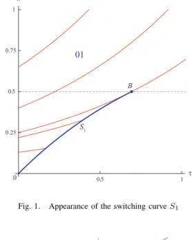
There is a switching curveS1that appears in the solution.
The switching condition for the first player is the following Au= (1−e−τ)(xz+1)−x(1−e−τ)z−x = (1−e−τ)−x = 0
Then
S1: x = 1 − e−τ
for x ≤ 12; indeed, the curve x = 1 − e−τ can only be
crossed by solutions ifx(T ) ≤ 1
4, which corresponds to an
intersection atx = 1 2.
First step of the construction of the characteristics is shown on Fig. 1. The blue line S1 is the switching curve for the
first player. Moving from the left side of S1 to the right
one the values πx and πτ are changing smoothly. But the
values ofνxandντ have a jump, because the corresponding
equation is changing. On the right side of it, the HJB-equation has the form
−ντ++ ν +
x(1 − x + xz) − V z + 1 = 0
where the+ superscript denotes the values “after” the jump in reverse time.
A normal vector to the switching surfaceS1 equals to
ν = ∇S1= (∂S1/∂x, ∂S1/∂τ ) = (−1, 1 − x)
Due to the continuity of the value function∇V+= ∇V−+
kν or µ ν+ x ν+ τ ¶ = µ ν− x ν− τ ¶ + k µ −1 1 − x ¶ = µ −k 1 + k(1 − x) ¶ with(ν− x, ν −
t ) = (0, 1). Substitution into the HJB-equation
gives k = − τ z 2(1 − x) + xz Then νx+= τ z 2(1 − x) + xz, ν + τ = 1 − (1 − x)τ z 2(1 − x) + xz 0.5 1 0.25 0.5 0.75 1 x τ 01 S 1 B 0
Fig. 1. Appearance of the switching curve S1
0.5 1 τ 0.25 x* 0.5 x 01 11 + future switch of v 0 A B 00 or a bisingular domain (?) a singular arc
Fig. 2. Possible optimal behavior of the players after the switch on S1
The argument in the Heaviside function of the second controlv becomes equal to
Av+ =
(2(1 − x)µ − (1 − 2x)z)τ 2(1 − x) + xz
The expression in the denominatorxz + 2(1 − x) is always positive sincex < 1/2 on S1. ThenAv+> 0 if 2(1 − x)µ −
(1−2x)z > 0 or x > x∗= (z −2µ)/2(z −µ). This holds for
all possiblex if z < 2µ. Otherwise there is an internal point x = x∗ such that A
v+ < 0 for 0 ≤ x < x∗ and Av+ > 0
forx∗< x ≤ 1/2.
The following situation corresponding to the valuesz = 8 andµ = 2 is shown on Fig. 2.
B. SegmentAB
Suppose that the coordinatex∗exists (0 < x∗< 1/2) and
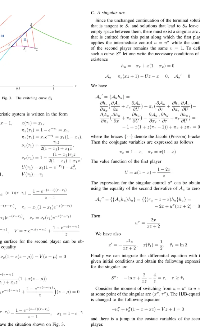
consider the characteristic field emitted from the segment AB. In addition let’s denote the coordinate of the switch on S1 as (x1, τ1). Both controls equals to one (predators are
0.5 1 τ 0.2 0.4 0.6 x A 11 01 B 0 C S 2
Fig. 3. The switching curve S2
and the characteristic system is written in the form x′ = −(z − 1)x − 1, x(τ1) = x1, π′ x= −πx, πx(τ1) = 1 − e−τ1 = x1, π′ τ = −πτz, πτ(τ1) = x1e−τ1 = x1(1 − x1), ν′ x= −νx, νx(τ1) = τ1z 2(1 − x1) + x1z , ν′ τ = −ντz, ντ(τ1) = 1 − (1 − x1)τ1z 2(1 − x1) + x1z , U′= −U z, U (τ 1) = x1(1 − e−τ1) = x21, V′= −V z + 1, V (τ 1) = τ1 Then x = x1e−(z−1)(τ −τ1)− 1 − e−(z−1)(τ −τ1) z − 1 πx= x1e−(τ −τ1), πτ= x1(1 − x1)e−z(τ −τ1) νx= νx(τ1)e−(τ −τ1), ντ= ντ(τ1)e−z(τ −τ1) U = x21e−z(τ −τ1), V = τ1e−z(τ −τ1)+ 1 − e−z(τ −τ1) z
The switching surface for the second player can be ob-tained from the equality
Av = νx(1 + x(z − µ)) − V (z − µ) = 0 or S2: τ1ze−(τ −τ1) 2(1 − x1) + x1z (1 + x(z − µ)) −³τ1e−z(τ −τ1)+ 1 − e−z(τ −τ1) z ´ (z − µ) = 0 where x = x1e−(z−1)(τ −τ1)− 1 − e−(z−1)(τ −τ1) z − 1 , x1= 1 − e −τ1
Finally, we have the situation shown on Fig. 3.
C. A singular arc
Since the unchanged continuation of the terminal solution that is tangent toS1 and solutions that lead to S2 leave an
empty space between them, there must exist a singular arcSσ
that is emitted from this point along which the first player applies the intermediate control u = uσ
while the control of the second player remains the same v = 1. To define such a curveSσ let one write the necessary conditions of its
existence hu= −πτ+ x(1 − πx) = 0 Au= πx(xz + 1) − U z − x = 0, Au′= 0 We have Au′ = {Auhu} = ∂hu ∂πx ¡ ∂ Au ∂x + πx ∂Au ∂U ¢ + πτ ¡ ∂ Au ∂τ + ∂hu ∂πτ ∂Au ∂U ¢− ∂Au ∂πx ¡ ∂ hu ∂x + πx ∂hu ∂U ¢ − ∂Au ∂πτ ¡ ∂ hu ∂τ + πτ ∂hu ∂U¢ = − 1 + x(1 + z(πx− 1)) + πx+ zπτ = 0
where the braces{· ·} denote the Jacobi (Poisson) brackets. Then the conjugate variables are expressed as follows
πx= 1 − x, πτ= x(1 − x)
The value function of the first player U = x(1 − x) +1 − 2x
z
The expression for the singular controluσ can be obtained
using the equality of the second derivative of Au to zero
Au′′= {{Auhu}hu} = {{(πx− 1 + x)hu}hu} = − 2x + uσ(xz + 2) = 0 Then uσ= 2x xz + 2 We have also x′ = − x2z xz + 2, x(˜τ1) = 1 2, τ˜1= ln 2
Finally we can integrate this differential equation with the given initial conditions and obtain the following expression for the singular arc
Sσ: − ln x + 2
xz − 4
z = τ, τ ≥ ˜τ1 Consider the moment of switching fromu = uσ
tou = 1 at some point of the singular arc(xσ, τσ). The HJB-equation
is changed to the following equation −νσ
τ + ν σ
x(1 − x + xz) − V z + 1 = 0
and there is a jump in the costate variables of the second player.
Along the singular arcSσ: V′= 1 − V zuσ= 1 − V 2xz xz + 2, x ′ = − x2z xz + 2, V (ln 2) = ln 2, x(ln 2) = 1 2 This can be rewritten in the form
dV dx = 2V xz − xz − 2 x2z , V (1/2) = ln 2 Therefore V = 4x2ln 2+(1 − 2x)(4 + 8x + 16x2+ 3xz(1 + 2x)) 6xz , V σ
Choose the variables = x as a parameter of the singular arc. In this case
∂τ ∂s = − 1 x− 2 x2z and ∂V ∂s = − 2 + 4x3(8 − 3z(2 ln 2 − 1)) 3x2z = ν σ x−ν σ τ µ 1 x+ 4 x2z 
After the substitution to the changed HJB-equation we have the following values of conjugate variables
νσ τ = 2 + 3xz + 4x3(8 − 3z(2 ln 2 − 1)) 6(xz + 1) , νσ x = 4 + 3xz − 4x3(8 − 3z(2 ln 2 − 1)) 6x(xz + 1)
These values are the initial conditions of characteristic trajectories emitted from the singular curveSσin the domain
11. For this domain we have again x′= −(z − 1)x − 1, x(τσ) = xσ, π′ x= −πx, πx(τσ) = 1 − xσ, π′ τ= −πτz, πτ(τσ) = xσ(1 − xσ), ν′ x= −νx, νx(τσ) = νxσ, ν′ τ = −ντz, ντ(τσ) = ντσ, U′= −U z, U (τσ) = xσ(1 − xσ) +1 − 2x σ z , V′= −V z + 1, V (τσ) = Vσ
The switching condition
Av = νx(1 + x(z − µ)) − V (z − µ) = 0 or Sσ 2: νxσe −(τ −τσ )(1 + x(z − µ))− µ Vσe−z(τ −τσ )+1 − e−z(τ −τ σ ) z ¶ (z − µ) = 0 where x = xσe−(z−1)(τ2−τ σ )−1 − e−(z−1)(τ2−τ σ ) z − 1
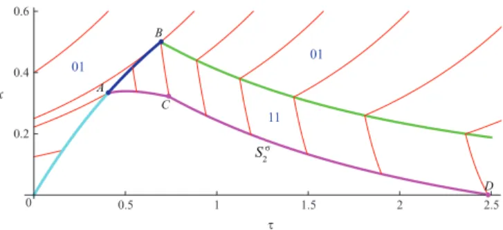
This curve is indicated on Fig. 4 by the segmentCD.
0.5 1 1.5 2 2.5 τ 0.2 0.4 0.6 x 0 B A C D 11 01 01 S 2 σ
Fig. 4. Construction of the switching curve Sσ 2
IV. BI-SINGULAR SOLUTION
A. Derivation of the Hamilton-Jacobi (HJ) equations
A simple Nash argument shows that it is not possible to have the region 00 inside the domain 0ACD (see Fig. 4). Indeed, let us consider the segment0A; in forward time, a solution initiated on the right of0A with the controls (0, 0) would be such that the predators only reproduce until the final time, while the preys first hide until reaching 0A and then eat until the final time. Obviously, the preys can improve their situation from there by instead choosing to eat all the time, since they are not threatened by the preadtors, which are reproducing. The controls(0, 0) can therefore not be part of a Nash solution on the right of 0A. Further analysis of A+u andA+v shows that no solution with bang-bang control
values can be emitted from0A.
The phenomenon of the appearance of the bi-singular solution for the class of nonzero-sum differential games has been recently investigated [6]. To define necessary equations for the value function in the bi-singular domain let one eliminate the controlsv and u from the pairs of the equations hu= −πτ− πxx(1 − µ(1 − v)) − µU (1 − v) + x = 0,
Au= πx(xz + 1)v − U vz − x = 0
hv = −ντ− νxx(1 − µ) − µV + 1 = 0,
Av= νx(u(xz + 1) − µx) + V (µ − uz) = 0
This leads to the following PDEs which are denoted HJ-equations (instead of the previous HJB-HJ-equations):
ˆ hu, −πτ− πxx(1 − µ) − µU + x − µx(πxx − U ) πx(xz + 1) − U z = 0 ˆ hv, −ντ− νxx(1 − µ) − µV + 1 = 0
The bi-singular controls can be obtained from the solution of these PDEs
uσ= µ(νxx − V )
νx(xz + 1) − V z
, vσ= x
πx(xz + 1) − U z
B. Solution of the second HJ-equation
Consider the HJ-equation regarding the second player ˆ
with singular control
uσ= µ(νxx − V )
νx(xz + 1) − V z
(0 ≤ uσ≤ 1)
The Characteristic system has the form x′ = −∂ˆhv ∂νx = −x(µ − 1), ν′ x= ∂ˆhv ∂x + νx ∂ˆhv ∂V = −νx, ν′ τ = ∂ˆhv ∂τ + ντ ∂ˆhv ∂V = −µντ, V′= −ν x ∂ˆhv ∂νx − ντ ∂ˆhv ∂ντ = −µV + 1, x(τ1) = x1, V (τ1) = τ1
If we take the segment 0A as the boundary we need to recalculate the values of the costate variables νx(τ1) and
ντ(τ1): µ νx(τ1) ντ(τ1) ¶ = µ −k 1 + k(1 − x) 
regarding the HJ-equation
−ντ(τ1) + νx(τ1)(µ − 1)x1− µτ1+ 1 = 0 Then k = − µτ1 µx1+ 1 − 2x1 and νx(τ1) = µτ1 µx1+ 1 − 2x1 , ντ(τ1) = 1 − (1 − x1)µτ1 µx1+ 1 − 2x1 Then x = x1e−(µ−1)(τ −τ1), νx= νx(τ1)e−(τ −τ1), ντ = ντ(τ1)e−µ(τ −τ1), V = τ1e−µ(τ −τ1)+1 − e −µ(τ −τ1) µ
By substitution of this solution we can write the expression for the singular controluσ. On the segment0A it equals to
uσ(τ 1) = µνx(τ1)x1− µτ1 νx(τ1)(x1z + 1) − τ1z = µ(1 − 2x1) (1 − 2x1)z − µ
which belongs to the interval between zero and one. The singular control equals exactly one at the boundary pointA:
uσ(τ 1) ¯ ¯ ¯x 1=x∗ = 1
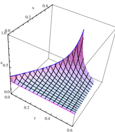
The result is shown on Fig. 5. The horizontal line forx = 0 is at leveluσ = µ/z.
Now let’s take the segmentAC into account. If we denote the coordinates of the point on AC as (x2, τ2) ∈ S2 and
corresponding to it the point onAB as (x1, τ1) we can write
x2= x1e−(z−1)(τ2−τ1)− 1 − e−(z−1)(τ2−τ1) z − 1 νx(τ2) = τ1ze−(τ2−τ1) 2(1 − x1) + x1z , 0.0 0.2 0.4 0.6 Τ 0.0 0.2 0.4 x 0.0 0.5 1.0 u
Fig. 5. Solution of the 2nd HJ-equation with a boundary at 0A
0.0 0.5 1.0 Τ 0.0 0.2 0.4 x 0.0 0.5 1.0 u
Fig. 6. Solution of the 2nd HJ-equation with a boundary at 0AC
ντ(τ2) = µ 1 − (1 − x1)τ1z 2(1 − x1) + x1z ¶ e−z(τ2−τ1) V (τ2) = τ1e−z(τ2−τ1)+ 1 − e−z(τ2−τ1) z withuσ(τ 2) = 1. Then x = x2e−(µ−1)(τ −τ2) νx= νx(τ2)e−(τ −τ2), ντ = ντ(τ2)e−µ(τ −τ2) V = V (τ2)e−µ(τ −τ2)+1 − e −µ(τ −τ2) µ
Using these expressions we can obtain the value of the singular controluσ
. The solution is shown on Fig. 6 by the set of blue curves started from the segmentAC. The surface closer to us indicates the previous solution.
The characteristics of the bi-singular field (which are not the game trajectories) intersect the field (11) coming, in backward time, from the singular arc. Therefore we can construct the singular line of the dispersal type such that Vσ = V11 on it, where the value Vσ denotes the solution
0.5 1 1.5 2 2.5 3 0.2 0.4 x 0 τ A C D E
Fig. 7. Final construction of the characteristic field for the 2nd HJ-equation
in the bi-singular domain, V11 – in the domain (11). This
gives the following construction shown on Fig. 7, where the dispersal line is indicated by the segment CE. The details of its construction are presented in the following subsection.
Construction of the dispersal lineCE
For one part of CE we should compare characteristics emitted from0A and characteristics emitted from the singu-lar arc. They will give a lower part ofCE. For another part we should consider the field (11) and bi-singular character-istics emitted from segmentAC.
For the characteristics from0A we have x11= x1e−(µ−1)(τ −τ1), V11= τ1e−µ(τ −τ1)+
1 − e−µ(τ −τ1)
µ for the characteristics fromAC
x11= x2e−(µ−1)(τ −τ2) V11= ³ τ1e−z(τ2−τ1)+1 − e −z(τ2−τ1) z ´ e−µ(τ −τ2) + 1 − e−µ(τ −τ2) µ where(τ1, x1) ∈ 0B and (τ2, x2) ∈ AC.
If we consider a primary domain we can write
xσ= xσe−(z−1)(τ −τ σ )−1 − e−(z−1)(τ −τ σ ) z − 1 , Vσ= 1 − e−z(τ −τσ ) z + e −z(τ −τσ )³4(xσ)2ln 2+ (1 − 2xσ)(4 + 8xσ+ 16(xσ)2+ 3xσz(1 + 2xσ)) 6xσz ´
where the coordinates (xσ, τσ) belong to the singular arc
Sσ.
The coordinates (τ3, x3) of the point on CF can be
obtained through equations V11 ¯ ¯ ¯τ=τ 3 = Vσ ¯ ¯ ¯τ=τ 3 andx11 ¯ ¯ ¯τ=τ 3 = xσ ¯ ¯ ¯τ=τ 3
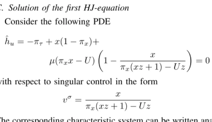
C. Solution of the first HJ-equation
Consider the following PDE ˆ hu= −πτ+ x(1 − πx)+ µ(πxx − U ) µ 1 − x πx(xz + 1) − U z ¶ = 0 with respect to singular control in the form
vσ= x
πx(xz + 1) − U z
The corresponding characteristic system can be written anal-ogously to the previous case
x′= −(µ − 1)x + µxU (πx(xz + 1) − U z)2 , π′ x= 1 − πx− µ(πxx − U ) πx(xz + 1) − U z , π′ τ = −µπτ µ 1 − πxx (πx(xz + 1) − U z)2 ¶ , U′ = x − µU −µx(U2z + πx2x(xz + 1) − 2U πx(xz + 1)) (πx(xz + 1) − U z)2
with initial condition on the segment0A
x(τ1) = x1, πτ(τ1) = x1(1−x1), πx(τ1) = x1, U (τ1) = x21 Notice that à ∂ ˜U ∂n !′ = (πxx − U )′= −µ(πxx − U )
But in our case(πxx − U )
¯ ¯ ¯τ=τ
1
= 0. Therefore πxx − U =
0 all the time. This leads to the characteristic equation for πx of the form πx′ = 1 − πx with initial condition on 0A:
α(τ1) = 1 − e−τ1= x1. Thenπx= 1 − e−τ and the singular
control can be written in the form directly depending onx andτ :
vσ= x
1 − e−τ
For the characteristic field emitted for the segmentAC the situation is more complicated since the conjugate variables have a jump on it. Suppose that the segmentS2 is defined
through the following conditions
S2: τ1ze−(τ −τ1) 2(1 − x1) + x1z (1 + x(z − µ)) − µ τ1e−z(τ −τ1)+ 1 − e−z(τ −τ1) z ¶ (z − µ) = 0 x = x1e−(z−1)(τ −τ1)− 1 − e−(z−1)(τ −τ1) z − 1 (x1= 1 − e −τ1)
Suppose that τ1 = τ1(x, τ ). If we differentiate the last
equation forx we obtain ∂τ1 ∂x = 1 − x1+ x1z (1 − x + xz)(2(1 − x1) + x1z) , ∂τ1 ∂τ = 1 − x1+ x1z 2(1 − x1) + x1z
0.2 A 0.6 C Τ 0.5 1 2 vΣ
Fig. 8. Singular control vσ
on the boundary of the bi-singular domain
To calculate the normal vector to S2 we need to calculate
the gradient
∇S2= (∂S2/∂x, ∂S2/∂τ )
Then we can derive the expressions for∂S2/∂x and ∂S2/∂τ
but we will omit this part since they have too complicated a form. Taking into account that
π+ x = x1e−(τ −τ1)+k ∂S2 ∂x , π + τ = x1(1−x1)e−z(τ −τ1)+k ∂S2 ∂τ we can substitute these values into the HJ-equation
−π+ τ+x(1−πx+)+µ(πx+x−U ) µ 1 − x πx+(xz + 1) − U z ¶ = 0 with U = x2
1e−z(τ −τ1) and obtain the equation w.r.t. the
scalar k. After that, we can write the new values of the conjugate variablesπ+
x andπ+τ.
We should notice that there are two possible solutionsk1
and k2. The value of k1 is negative on AC and equals to
zero at pointA. But this branch corresponds to the situation when vσ ≥ 1. Another branch of the solution with k
2 > 0
corresponds to the valuesvσ∈ (0, 1), see Fig. 8.
The resulting characteristic field for the segment0A and AC is shown on Fig. 9.
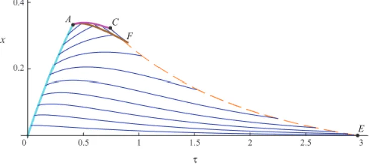
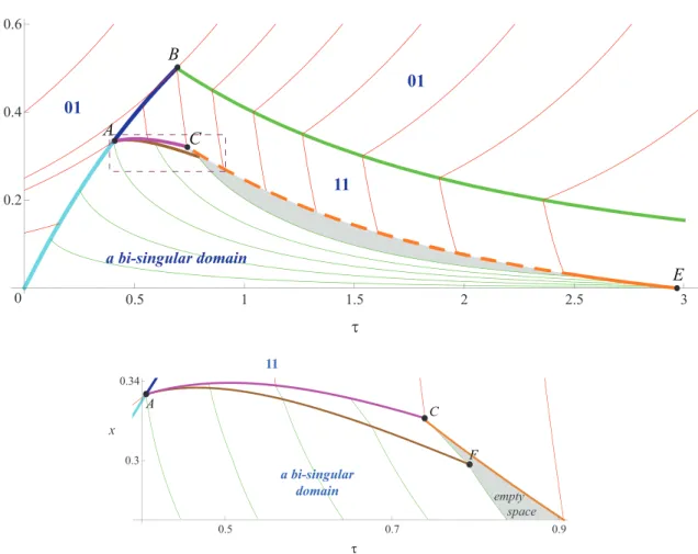
D. Construction of the real game trajectories
Using the constructed solution of the decomposed system of two HJ-equations, we can compute the pair of singular controls uσ and vσ in the domain 0ACE. Thus, we can
construct the real game trajectories in the bi-singular domain. They are shown on Fig. 10. We can identify our main difficulty on this figure. Even though the whole space was filled with the characteristics for the decomposed system of two HJ equations, there is an empty subdomain in the final portrait of optimal trajectories (shaded area of Figure 10). This is a strong indication that some important things may have been missed in the process of deriving the solution.
V. CONCLUSIONS
We did not finalize the solution and did not cover the whole phase space by the field of characteristics. But our work is still in progress and we will continue our research. Nevertheless, we would like to point out that in the paper we investigated the transition from bang-bang controls to bi-singular ones and apply the method of characteristics to a
0.5 1 1.5 2 2.5 3 0.2 0.4 x 0 τ A C E F
Fig. 9. Characteristic field for the first HJ-equation
system of two HJB-equations. Although the fact that we did not find the solution in a subdomain of the phase space can be crucial and a new idea of the solution can change the whole picture drastically we think that the proposed solution will remain fulfilled in a sufficiently large area of the phase space after.
The theory of nonzero-sum differential games is not well-developed yet. There are no theorems of existence and uniqueness of their solution [6], [7], [8] so that it might be possible that no Nash equilibrium exist from the initial states in the ”void” zone. There might also be several, may be an infinity, of Nash equilibria. There is no strict classification of possible singular surfaces as one has been done for zero-sum differential games, see for example [9, p. 121]. Therefore this work is only an attempt to study a particular nonzero-sum differential games with an application in behavioral ecology.
VI. ACKNOWLEDGMENTS
This research has been supported by the ’Lutins&Co’ COLOR project of INRIA Sophia Antipolis-M´editerran´ee and the ’IA2L’ project of the SPE department of INRA. The work of the first author has been partially supported by the Russian Foundation for Basic Research (grant 07-04-00418).
REFERENCES
[1] S. A. H. Geritz and E. Kisdi, On the mechanistic underpinning of discrete-time population models with complex dynamics, Journal of
Theoretical Biology, vol. 228, 2004, pp 261-269.
[2] W. W. Murdoch, C. J. Briggs and R. M. Nisbet, Consumer-resource
dynamics., Princeton University Press, Princeton, NJ; 2003. [3] E. Pachepsky, R. M. Nisbet and W. W. Murdoch, Between discrete and
continuous consumer-resource dynamics with synchronized reproduc-tion, Ecology, vol. 89(1), 2008, pp 280-288.
[4] A. R. Akhmetzhanov, F. Grognard and L. Mailleret, Long term prey-predator dynamics induced by short term optimal prey-predatory behavior,
In preparation
[5] A. Friedman, Differential Games, Wiley-Interscience; 1971. [6] F. Hamelin and P. Bernhard, Uncoupling Isaacs equations in
two-player nonzero-sum differential games. Parental conflict over care as an example, Automatica, vol. 44(3), 2008, pp 882-885.
[7] P. Cardaliaguet and S. Plaskacz, Existence and uniqueness of a Nash equilibrium feedback for a simple non-zero-sum differential game,
International Journal of Game Theory, vol. 32(1), 2003, pp 33-71. [8] A. Bressan and W. Shen, Semi-cooperative strategies for differential
games, International Journal of Game Theory, vol. 32(4), 2004, pp 561-593.
[9] A. A. Melikyan, Generalized characteristics of first order PDEs:
applications in optimal control and differential games, Birh¨auser, Boston; 1998.
0.5 1 1.5 2 2.5 3 0.2 0.4 0.6