HAL Id: hal-01518713
https://hal.archives-ouvertes.fr/hal-01518713
Submitted on 5 May 2017
HAL is a multi-disciplinary open access
archive for the deposit and dissemination of
sci-entific research documents, whether they are
pub-lished or not. The documents may come from
teaching and research institutions in France or
abroad, or from public or private research centers.
L’archive ouverte pluridisciplinaire HAL, est
destinée au dépôt et à la diffusion de documents
scientifiques de niveau recherche, publiés ou non,
émanant des établissements d’enseignement et de
recherche français ou étrangers, des laboratoires
publics ou privés.
Location-domination on Interval and Permutation
Graphs
Florent Foucaud, George Mertzios, Reza Naserasr, Aline Parreau, Petru
Valicov
To cite this version:
Florent Foucaud, George Mertzios, Reza Naserasr, Aline Parreau, Petru Valicov. Algorithms and
Complexity for Metric Dimension and Location-domination on Interval and Permutation Graphs.
International Workshop on Graph-Theoretic Concepts in Computer Science WG 2015, Jun 2015,
Munich, Germany. pp.175 - 471, �10.1007/978-3-662-53174-7_32�. �hal-01518713�
and Location-Domination on Interval and
Permutation Graphs
⋆Florent Foucaud1, George Mertzios2⋆⋆, Reza Naserasr3, Aline Parreau4, and
Petru Valicov5
1
Université Blaise Pascal, LIMOS - CNRS UMR 6158, Clermont-Ferrand (France) [email protected]
2
School of Engineering and Computing Sciences, Durham University (UK) [email protected]
3
CNRS, Université Paris-Sud 11, LRI - CNRS UMR 8623, Orsay (France) [email protected]
4
CNRS, Université de Lyon 1, LIRIS - CNRS UMR 5205 (France) [email protected]
5
LIF - CNRS UMR 7279, Université d’Aix-Marseille (France) [email protected]
Abstract. We study the problems Locating-Dominating Set and Metric Dimension, which consist of determining a minimum-size set of vertices that distinguishes the vertices of a graph using either neigh-bourhoods or distances. We consider these problems when restricted to interval graphs and permutation graphs. We prove that both decision problems are NP-complete, even for graphs that are at the same time interval graphs and permutation graphs and have diameter 2. While Locating-Dominating Setparameterized by solution size is trivially fixed-parameter-tractable, it is known that Metric Dimension is W [2]-hard. We show that for interval graphs, this parameterization of Metric Dimensionis fixed-parameter-tractable.
1
Introduction
Combinatorial identification problems have been widely studied in various con-texts. The common characteristic of these problems is that we are given a combi-natorial structure, and we wish to distinguish (i.e. uniquely identify) its elements by the means of a small set of selected elements. In this paper, we study two such identification problems where the instances are graphs. In the
Locating-Dominating Setproblem, we ask for a dominating set S such that the vertices
outside of S are distinguished by their neighbourhood within S. In Metric
Di-mension, we wish to select a set S of vertices of a graph G such that every
vertex of G is uniquely identified by its distances to the vertices of S.
⋆
This is a short version of the full paper [16] available on arXiv:1405.2424.
⋆⋆
These problems have been extensively studied since their introduction in the 1970s and 1980s. They have been applied to various areas such as network verification [2], fault-detection in networks [36], graph isomorphism testing [1] or the logical definability of graphs [26].
Important concepts and definitions. All considered graphs are connected, finite and simple. We denote by N [v], the closed neighbourhood of vertex v, and by N (v) its open neighbourhood, i.e. N [v] \ {v}. A vertex is universal if it is adjacent to all the vertices of the graph. A set S of vertices of G is
a dominating set if for every vertex v, there is a vertex x in S ∩ N [v]. In
the context of dominating sets we say that a vertex x separates two distinct vertices u, v if it dominates exactly one of them. Set S separates the vertices of a set X if all pairs of X are separated by a vertex of S. Given a partial set S, we say that two distinct vertices u, v need to be separated if S does not separate them. If the set S is clear from context, then we simply say x, y need to be separated. The distance between two vertices u, v is denoted d(u, v). The following two definitions are the main concepts studied in this paper. • (Slater [33,34]) A set L of vertices of a graph G is a locating-dominating set if it is a dominating set and it separates the vertices of V (G) \ L.
• (Harary and Melter [21], Slater [32]) A set R of vertices of a graph G is a resolving set if for each pair u, v of distinct vertices, there is a vertex x of R with d(x, u) 6= d(x, v).
The smallest size of a locating-dominating set of G is the location-domination number of G, denoted γLD(G). The smallest size of a resolving set of G is the
metric dimension of G, denoted dim(G). The inequality dim(G) ≤ γLD(G),
relating these notions, holds for every graph G. If G has diameter 2, the two concepts are almost the same, as then, one can check that γLD(G) ≤ dim(G) + 1 holds. We consider the two associated decision problems:
Locating-Dominating Set Instance: A graph G, an integer k. Question: Is it true that γLD(G) ≤ k?
Metric Dimension
Instance: A graph G, an integer k. Question: Is it true that dim(G) ≤ k? We will study these problems on interval graphs and permutation graphs, which are classic graph classes that have many applications and are widely stud-ied. They can be recognized efficiently, and many problems can be solved effi-ciently for graphs in these classes (see e.g. the book by Golumbic [19]). Given a set S of (geometric) objects, the intersection graph G of S is the graph whose vertices are associated to the elements of S and where two vertices are adjacent if and only if the corresponding elements of S intersect. Then, S is called an intersection model of G. An interval graph is the intersection graph of a set of (closed) intervals of the real line. Given two parallel lines B and T , a permutation graph is the intersection graph of segments of the plane which have one endpoint on B and the other endpoint on T .
Previous work. The complexity of distinguishing problems has been studied by many authors. Locating-Dominating Set was first proved to be NP-complete in [7], a result extended to bipartite graphs in [5]. This was improved to
pla-nar bipartite unit disk graphs [29] and to plapla-nar bipartite subcubic graphs [14].
Locating-Dominating Setis hard to approximate within any o(log n) factor
(n is the order of the graph), with no restriction on the input graph [35]. This re-sult was extended to bipartite graphs, split graphs and co-bipartite graphs [14]. On the positive side, Locating-Dominating Set is constant-factor approx-imable for bounded degree graphs [20], line graphs [14,15], interval graphs [4] and is linear-time solvable for graphs of bounded clique-width (using Courcelle’s theorem [8]). Furthermore, an explicit linear-time algorithm solving
Locating-Dominating Seton trees is known [33].
Metric Dimension, which has a non-local and more intricate flavour, was
widely studied as well, and has (re)gained a lot of attention within the last few years. It was shown NP-complete in [18, Problem GT61]. This result has re-cently been extended to bipartite graphs, co-bipartite graphs, split graphs and line graphs of bipartite graphs [11], to a special subclass of unit disk graphs [24], and to planar graphs [9]. Polynomial-time algorithms for the weighted version of Metric Dimension for paths, cycles, trees, graphs of bounded cyclomatic number, cographs and partial wheels were given in [11]. A polynomial-time algo-rithm for outerplanar graphs was designed in [9] and one for chain graphs in [12]. It was shown in [2] that Metric Dimension is hard to approximate within any o(log n) factor for graphs of order n. This is even true for bipartite subcubic graphs, as shown in [22,23].
In light of these results, the complexity of Locating-Dominating Set and
Metric Dimensionfor interval and permutation graphs is a natural open
ques-tion (as posed in [28] and [11] for Metric Dimension on interval graphs), since these classes are standard candidates for designing efficient algorithms.
Let us say a few words about the parameterized complexity of these problems. For standard definitions and concepts in parameterized complexity, we refer to the books [10,30]. It is known that for Locating-Dominating Set, any graph of order n and solution size k satisfies n ≤ 2k+k−1 [34]. Therefore, when
param-eterized by k, Locating-Dominating Set is trivially fixed-parameter-tractable (FPT): first check whether the above inequality holds (if not, return “no”), and if yes, use a brute-force algorithm checking all possible subsets of vertices. This is an FPT algorithm. However, Metric Dimension (again parameterized by solution size k) is W[2]-hard even for bipartite subcubic graphs [22,23].
Remar-quably, the bound n ≤ Dk + k holds [6] (where n is the graph’s order, D its
diameter, and k is the size of a resolving set). Hence, for graphs of diameter bounded by a function of k, the same arguments as the previous ones yield an FPT algorithm for Metric Dimension. This holds, for example, for the class of (connected) split graphs, which have diameter at most 3. Besides this, as re-marked in [23], no standard class of graphs for which Metric Dimension is FPT was previously known.
Our results. We settle the complexity of Locating-Dominating Set and
Metric Dimensionon interval and permutation graphs, showing that the two
problems are NP-complete even for graphs that are at the same time inter-val graphs and permutation graphs and have diameter 2 (Section 2). Then, we
present a dynamic programming algorithm (using path-decomposition) to solve
Metric Dimension in FPT time on interval graphs (Section 3). Up to our
knowledge, this is the first nontrivial FPT algorithm for this problem. Due to space constraints, some proofs are deferred to the full version of the paper [16].
2
Hardness results
We will now reduce 3-Dimensional Matching, which is a classic NP-complete problem [25], to Locating-Dominating Set on interval graphs.
3-Dimensional Matching
Instance: Three disjoint sets A, B and C each of size n, and a set T of m triples of A × B × C.
Question: Is there a perfect 3-dimensional matching M ⊆ T of the hypergraph (A ∪ B ∪ C, T ), i.e. a set of disjoint triples of T such that each element of A ∪ B ∪ C belongs to exactly one of the triples?
2.1 Preliminaries and gadgets
We first define the following dominating gadget (a path on four vertices). The idea is to ensure that specific vertices are dominated locally, and therefore sep-arated from the rest of the graph. We will use it extensively. The reduction is described as an interval graph, but we then show that it is also a permutation graph. In all that follows, we always consider interval graphs with an interval representation.
Definition 1 (Dominating gadget). A dominating gadget D is a subgraph of an interval graph G inducing a path on four vertices, and such that each interval of V (G) \ V (D) either contains all intervals of V (D) or does not intersect any. In the following, a dominating gadget will be represented as in Figure 1(a).
D
(a) Dominating gadget D.
u
v D(uv)
(b) Choice pair u, v. Fig. 1.Representations of dominating gadget and choice pair.
The following claim is easy to observe.
Claim 2. If G is an interval graph containing a dominating gadget D and S is a locating-dominating set of G, then |S ∩ V (D)| ≥ 2.
If x1, x2, x3, x4 denote the vertices of D, the set SD = {x1, x4} is called the
standard solution for D. It is a locating-dominating set of D and if S is an optimal locating-dominating set of G, then replacing S ∩ V (D) by the standard solution SD, one can obtain an optimal locating-dominating set S′.
Definition 3 (Choice pair). A pair {u, v} of intervals is called a choice pair if u, v both contain the intervals of a common dominating gadget (denoted D(uv)), and such that none of u, v contains the other.
See Figure 1(b) for an illustration of a choice pair. Intuitively, a choice pair gives us the choice of separating it from the left or from the right: since none of u, v is included in the other, the intervals intersecting u but not v can only be located at one side of u; the same holds for v. In our construction, we will make sure that, except for the choice pairs, all pairs of intervals will be easily separated using domination gadgets. Our aim will then be to separate the choice pairs. We have the following claim that follows directly from Claim 2:
Claim 4. Let S be a locating-dominating set of an interval graph G and {u, v} be a choice pair in G. If the solution S ∩ V (D(uv)) for the dominating gadget D(uv) is the standard solution, both vertices u and v are dominated, separated from all vertices in D(uv) and from all vertices not intersecting D(uv).
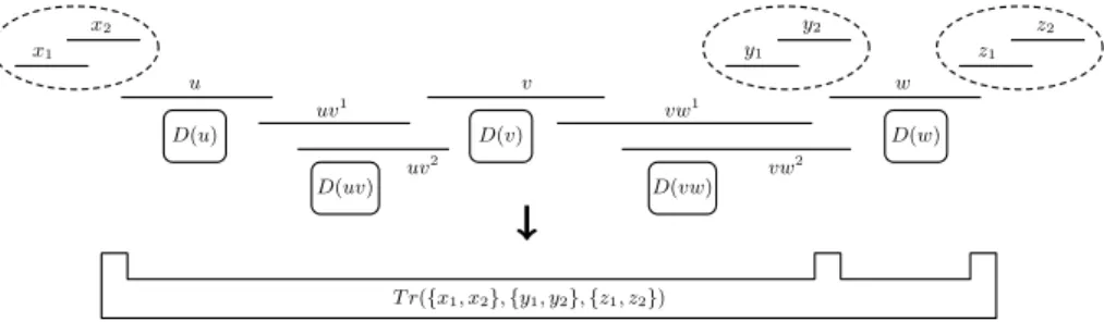
We now define the central gadget of the reduction, the transmitter gadget. Roughly speaking, it allows to transmit information across an interval graph. Definition 5 (Transmitter gadget). Let P be a set of two or three choice pairs in an interval graph G. A transmitter gadget T r(P ) is a subgraph of G consisting of a path on seven vertices {u, uv1, uv2, v, vw1, vw2, w} and five
dom-inating gadgets D(u), D(uv), D(v), D(vw), D(w) such that the following prop-erties are satisfied:
• u and w are the only vertices of T r(P ) that separate the pairs of P .
• The intervals of the dominating gadget D(u) (resp. D(v), D(w)) are included in interval u (resp. v, w) and no interval of T r(P ) other than u (resp. v, w) intersects D(u) (resp. D(v), D(w)).
• Pair {uv1, uv2} is a choice pair and no interval of T r(P ) \ (D(uv1, uv2) ∪
{uv1, uv2}) intersects both intervals of the pair. The same holds for pair
{vw1, vw2}.
• The choice pairs {uv1, uv2} and {vw1, vw2} cannot be separated by intervals
of G other than u, v and w.
Figure 2 illustrates a transmitter gadget and shows the succinct graphical representation that we will use. As shown in the figure, we may use a “box” to denote Tr(P ). This box does not include the choice pairs of P but indicates where
they are situated. Note that the middle pair {y1, y2} could also be separated
(from the left) by u instead of w, or it may not exist at all if P contains only two pairs.
The following claim shows how transmitter gadgets will be used in the main reduction.
Claim 6. Let G be an interval graph with a transmitter gadget T r(P ) and let S be a locating-dominating set of G. We have |S ∩T r(P )| ≥ 11 and if |S ∩T r(P )| = 11, then no pair of P is separated by a vertex in S ∩T r(P ). Moreover, there exist two sets of vertices of T r(P ), S−
T r(P ) and S +
such that the following holds:
• The set ST r(P )− dominates all the vertices of T r(P ) and separates all the pairs of T r(P ) but no pairs in P .
• The set ST r(P )+ dominates all the vertices of T r(P ), separates all the pairs of T r(P ) and all the pairs in P .
Proof. By Claim 2, we must have |S∩T r(P )| ≥ 10 with 10 vertices of S belonging to the dominating gadgets. In order that uv1, uv2 are separated, at least one
vertex of {u, uv1, uv2, v} belongs to S (recall that by definition the intervals
not in T r(P ) cannot separate the choice pairs in T r(P )), and similarly, for the choice pair {vw1, vw2}, at least one vertex of {v, vw1, vw2, w} belongs to S.
Hence |S ∩ T r(P )| ≥ 11 and if |S ∩ T r(P )| = 11, vertex v must be in S and neither u nor w are in S. Therefore, no pair of P is separated by a vertex in S ∩ T r(P ).
We now prove the second part of the claim. Let Sdom be the union of the
five standard solutions SD of the dominating gadgets of T r(P ). Let ST r(P )− =
Sdom∪ {v} and S+T r(P ) = Sdom∪ {u, w}. The set Sdom has 10 vertices and so
ST r(P )− and S+T r(P )have respectively 11 and 12 vertices. Each interval of T r(P ) either contains a dominating gadget or is part of a dominating gadget and is therefore dominated by a vertex in Sdom. Hence, pairs of vertices that are not
intersecting the same dominating gadget are clearly separated. By Claim 2, no vertex in a dominating gadget D is dominated by all vertices of SD, hence a
vertex adjacent to the whole of D is separated from all the vertices of D. Also, by Claim 2, all pairs of vertices inside a dominating gadget are separated by Sdom. Therefore, the only remaining pairs to consider are the choice pairs. Note
that they are separated both at the same time either by v or by {u, w}. Hence the two sets ST r(P )− and S+T r(P )are both dominating and separating the vertices of T r(P ). Moreover, since ST r(P )+ contains u and w, it also separates the pairs
of P . ⊓⊔
We will call the sets ST r(P )− and S+T r(P ) the tight and non-tight standard solutions of T r(P ). x1 x2 u uv1 uv2 v y1 y2 vw1 vw2 w z1 z2 D(u) D(uv) D(v) D(vw) D(w) T r({x1, x2}, {y1, y2}, {z1, z2})
2.2 The main reduction
We now describe the reduction. Each element x ∈ A ∪ B ∪ C is modelled by a choice pair{fx, gx}. Each triple of T is modelled by a triple gadget:
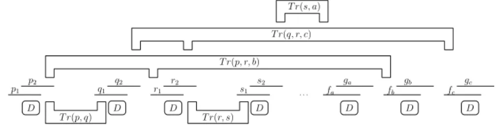
Definition 7 (Triple gadget). Let T = {a, b, c} be a triple of T . The triple gadget Gt(T ) is an interval graph consisting of four choice pairs p = {p1, p2},
q = {q1, q2}, r = {r1, r2}, s = {s1, s2} together with their associated dominating
gadgets D(p), D(q), D(r), D(s) and five transmitter gadgets T r(p, q), T r(r, s), T r(s, a), T r(p, r, b) and T r(q, r, c), where:
• a = {fa, ga}, b = {fb, gb} and c = {fc, gc};
• Except for the choice pairs, for each pair of intervals of Gt(T ), its two intervals
intersect different subsets of {D(p), D(q), D(r), D(s)};
• In each transmitter gadget T r(P ) and for each choice pair π ∈ P , the intervals of π intersect the same intervals except for the vertices u, v, w of T r(P ); • The intervals of V (G)\V (Gt(T )) that are intersecting only a part of the gadget
intersect according to the transmitter gadget definition and do not separate the choice pairs p, q, r and s.
An illustration of a triple gadget is given in Figure 3. We remark that p, q, r and s in Gt({a, b, c}), are all functions of {a, b, c} but to simplify the notations
we simply write p, q, r and s.
The proof of the following claim is similar to the proof of Claim 6.
Claim 8. Let G be a graph with a triple gadget Gt(T ) and S be a
locating-dominating set of G. We have |S ∩ Gt(T )| ≥ 65 and if |S ∩ Gt(T )| = 65, no
choice pair corresponding to a, b or c is separated by a vertex in S ∩ Gt(T ).
Moreover, there exist two sets of vertices of Gt(T ), SG−t(T )and SG+t(T ) of size 65
and 66 respectively, such that the following holds.
• The set SG−t(T ) dominates all the vertices of Gt(T ) and separates all the pairs
of Gt(T ) but does not separate any choice pairs corresponding to {a, b, c}.
• The set SG+t(T ) dominates all the vertices of Gt(T ), separates all the pairs of
Gt(T ) and separates the choice pairs corresponding to {a, b, c}.
p1 p2 q1 q2 r1 r2 s1 s2 fa ga fb gb fc gc . . . D D D D D D D T r(p, q) T r(r, s) T r(p, r, b) T r(q, r, c) T r(s, a)
Fig. 3.Triple gadget Gt(T ) with T = {a, b, c} together with the choice pairs of elements
a, b and c. We recall that these choice pairs and their dominating gadgets are not part of Gt(T ).
Given an instance (A, B, C, T ) of 3-Dimensional Matching with |A| = |B| = |C| = n and |T | = m, we construct the interval graph G = G(A, B, C, T ) as follows.
• As mentioned previously, to each element x of A ∪ B ∪ C, we assign a dis-tinct choice pair {fx, gx} in G. The intervals of any two distinct choice pairs
{fx, gx}, {fy, gy} are disjoint and they are all in R+.
• For each triple T = {a, b, c} of T we first associate an interval IT in R− such
that for any two triples T1 and T2, IT1 and IT2 do not intersect
6
. Then inside IT, we build the choice pairs {p1, p2}, {q1, q2}, {r1, r2}, {s1, s2}. Finally, using
the choice pairs already associated to elements a, b and c we complete this to a triple gadget.
• When placing the remaining intervals of the triple gadgets, we must ensure that triple gadgets do not “interfere”: for every dominating gadget D, no interval in V (G) \ V (D) must have an endpoint inside D. Similarly, the choice pairs of each triple gadget or transmitter gadget must only be separated by intervals among u, v and w of its corresponding private transmitter gadget. For intervals of dis-tinct triple gadgets, this is easily done by our placement of the triple gadgets. To ensure that the intervals of transmitter gadgets of the same triple gadget do not interfere, we proceed as follows. We place the whole gadget T r(p, q) inside interval u of T r(p, r, b). Similarly, the whole T r(r, s) is placed inside interval v of T r(p, r, b) and w of T r(q, r, c). One has to be more careful when placing the intervals of T r(p, r, b) and T r(q, r, c). In T r(p, r, b), we must have that interval u separates p from the right of p. We also place u so that it separates r from the left of r. Intervals uv1, uv2both start in r
1, so that u also separates uv1, uv2
without these intervals interfering with the ones of r. Intervals uv1, uv2continue
until after pair s. In T r(q, r, c), we place u so that it separates q from the right, and we place w so that it separates r from the right; intervals uv1, uv2, v lie
strictly between q and r; intervals vw1, vw2 intersect r
1, r2 but stop before the
end of r2 (so that w can separate both pairs vw1, vw2 and r but without these
pairs interfering). It is now easy to place T r(s, a) between s and a.
The graph G(A, B, C, T ) has 159m + 18n vertices and the interval represen-tation described by our procedure can be obtained in polynomial time. We are now ready to state the main result of this section.
Theorem 9. (A, B, C, T ) has a perfect 3-dimensional matching if and only if G = G(A, B, C, T ) has a locating-dominating set with 65m + 7n vertices.
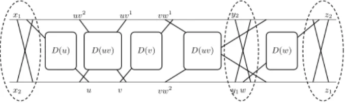
Theorem 9 shows that Locating-Dominating Set is NP-complete for in-terval graphs. In fact, one can prove that the constructed graph G(A, B, C, T ) is also a permutation graph, see for example Figure 4 for an illustration of the transmitter gadget as a permutation diagram intersection model.
Corollary 10. Locating-Dominating Set is NP-complete for graphs that are both interval and permutation graphs.
6
x1 x2 u D(u) uv1 uv2 D(uv) v D(v) vw2 vw1 D(uv) w D(w) y2 y1 z1 z2
Fig. 4.Permutation diagram intersection model of a transmitter gadget.
2.3 Diameter 2 and consequence for Metric Dimension
We now describe a self-reduction for Locating-Dominating Set for graphs with a universal vertex (hence, graphs of diameter 2), and a similar reduction from Locating-Dominating Set to Metric Dimension.
Let G be a graph. Let f1(G) be the graph obtained from G by adding a
universal vertex u and a neighbour v of u of degree 1. Let f2(G) be the graph
obtained from G by adding two adjacent universal vertices u, u′ and two
non-adjacent vertices v and w that are only non-adjacent to u and u′. See Figure 5 for
an illustration. One can show that γLD(f
1(G)) = γLD(G) + 1, and dim(f2(G)) = γLD(G) + 2. G u v f1(G) G u u′ v w f2(G)
Fig. 5.Two reductions for diameter 2.
This implies the following two theorems.
Theorem 11. Let C be a class of graphs that is closed under the graph
trans-formation f1. If Locating-Dominating Set is NP-complete for graphs in C,
then it is also NP-complete for graphs in C that have diameter 2.
Theorem 12. Let C be a class of graphs that is closed under the graph
transfor-mation f2. If Locating-Dominating Set is NP-complete for graphs in C, then
Metric Dimensionis also NP-complete for graphs in C that have diameter 2.
Since Theorems 11 and 12 can be applied to interval graphs and permutation graphs, Corollary 10 implies the following.
Corollary 13. Locating-Dominating Set and Metric Dimension are NP-complete for diameter 2-graphs that are both interval and permutation graphs.
3
Metric Dimension
is FPT on interval graphs
We now prove that Metric Dimension (parameterized by solution size) is FPT on interval graphs. The algorithm is based on dynamic programming over a path-decomposition.
Given an interval graph G, we can assume that in its interval model, all endpoints are distinct, and that the intervals are closed. We define two natural total orderings of V (G) based on this model: x <L y if and only if the left
endpoint of x is smaller then the left endpoint of y, and x <R y if and only if
the right endpoint of x is smaller than the right endpoint of y. We will work with the fourth distance-power G4of the input graph G which is also an interval
graph and has an interval model inducing the same orders <Land <Ras G [17].
Our algorithm will use dynamic programming on anice path-decomposition
of G4. The classic concepts of tree-decompositions and its “nice” variant, due to
Kloks [27].
Definition 14. A tree-decomposition of a graph G is a pair (T , X ), where T is a tree and X := {Xt : t ∈ V (T )} is a collection of subsets of V (G) (called
bags), and they must satisfy the following conditions: (i)St∈V (T )Xt= V (G);
(ii) for every edge uv ∈ E(G), there is a bag of X that contains both u and v; (iii) for every vertex v ∈ V (G), the set of bags containing v induces a connected subtree of T .
Given a tree-decomposition of (T , X ), the maximum size of a bag Xtover all
tree nodes t of T minus one is called the width of (T , X ). The minimum width of a tree-decomposition of G is the treewidth of G. The notion of tree-decomposition has been used extensively in algorithm design, especially via dynamic program-ming over the tree-decomposition.
We consider arooted tree-decomposition by fixing a root of T and orienting the tree edges from the root toward the leaves. A rooted tree-decomposition is nice (see Kloks [27]) if each node t of T has at most two children and falls into one of the four types:
(i)Join node: t has exactly two children t1and t2, and Xt= Xt1 = Xt2.
(ii)Introduce node: t has a unique child t′, and X
t= Xt′∪ {v}. (iii)Forget node: t has a unique child t′, and X
t= Xt′\ {v}. (iv)Leaf node: t is a leaf node in T .
Given a tree-decomposition, a nice tree-decomposition of the same width always exists and can be computed in linear time [27].
If G is an interval graph, we can construct a tree-decomposition of G (in fact, a path-decomposition) with special properties.
Proposition 15. Let G be an interval graph with clique number ω and an in-terval model inducing orders <L and <R. Then, G has a nice tree-decomposition
(P, X ) of width ω − 1 that can be computed in linear time, where moreover: (a) P is a path (hence there are no join nodes);
(b) every bag is a clique;
(c) going through P from the leaf to the root, the order in which vertices are introduced in an introduce node corresponds to <L;
(d) going through P from the leaf to the root, the order in which vertices are forgotten in a forget node corresponds to <R;
Proof. Given a graph G, one can decide if it is an interval graph and, if so, compute a representation of it in linear time [3]. This also gives us the ordered set of endpoints of intervals of G.
To obtain (P, X ), we first create the leaf node t, whose bag Xtcontains the
interval with smallest left endpoint. We then go through the set of all endpoints of intervals of G, from the second smallest to the largest. Let t be the last created node. If the new endpoint is a left endpoint ℓ(I), we create an introduce node t′ with X
t′ = Xt∪ {I}. If the new endpoint is a right endpoint r(I), we create
a forget node t′ with X
t′ = Xt\ {I}. In the end we create the root node as a
forget node t with Xt= ∅ that forgets the last interval of G.
Observe that one can associate to every node t (except the root) a point p of the real line, such that the bag Xt contains precisely the set of intervals
containing p: if t is an introduce node, p is the point ℓ(I) associated to the creation of t, and if t is a forget node, it is the point r(I)+ǫ, where ǫ is sufficiently small and r(I) is the endpoint associated to the creation of t. This set forms a clique, proving Property (b). Furthermore this implies that the maximum size of a bag is ω, hence the width is at most ω − 1 (and at least ω − 1 since every clique must be included in some bag).
Moreover it is clear that the procedure is linear-time, and by construction, Properties (a), (c), (d), (e) are fulfilled.
Let us now show that (P, X ) is a tree-decomposition. It is clear that every vertex belongs to some bag, proving Property (i) of Definition 14. Moreover let u, v be two adjacent vertices of G, and assume u <L v. Then, consider the
introduce node of P where v is introduced. Since u has started before v but has not stopped before the start of v, both u, v belong to Xt, proving Property (ii).
Finally, note that a vertex v appears exactly in all bags starting from the bag where v is introduced, until the bag where v is forgotten. Hence Property (iii) is
fulfilled, and the proof is complete. ⊓⊔
Lemma 16. Let G be an interval graph with an interval model inducing orders <L and <R, let d ≥ 1 be an integer and let (P, X ) be a tree-decomposition
of Gd obtained by Proposition 15 (recall that Gd is an interval graph, and it
has an intersection model inducing the same orders <L and <R[17]). Then the
following holds.
(a) Let t be an introduce node of (P, X ) with child t′, with X
t = Xt′ ∪ {v}. Then, Xt contains every vertex w in G such that dG(v, w) ≤ d and w <Lv.
(b) Let t′ be the child of a forget node t of (P, X ), with X
t= Xt′\ {v}. Then, Xt′ contains every vertex w in G such that dG(v, w) ≤ d and v <Rw.
We now present the most crucial preliminary results necessary for our al-gorithm. We first start with a definition related to the linear structure of an interval graph that we will use extensively.
Definition 17. Given a vertex u of an interval graph G, the rightmost path PR(u) of u is the path uR0, . . . , uRp where u = uR0, for every uRi (i ∈ {0, . . . , p−1})
uR
i+1 is the neighbour of uRi with the largest right endpoint, and thus u R p is the
PL(u) = uL0, . . . , uLq where for every u L
i (i ∈ {0, . . . , q − 1}) u L
i+1 is the neighbour
of uL
i with the smallest left endpoint.
Note that PR(u) and PL(u) are two shortest paths from u to uRp and u L q,
respectively. We say that a pair u, v of intervals in an interval graph G is sep-arated by interval x strictly from the right (strictly from the left, respectively) if x starts after both right endpoints of u, v (ends before both left endpoints of u, v respectively). In other words, x is not a neighbour of any of u and v.
The next lemma is crucial for our algorithm.
Lemma 18. Let u, v, x be three intervals in an interval graph G and let i be an integer such that x starts after both right endpoints of uR
i ∈ PR(u) and
vR
i ∈ PR(v). Then the three following facts are equivalent:
(1) x separates uR i, vRi ;
(2) for every j with 0 ≤ j ≤ i, x separates uR j, vjR;
(3) for some j with 0 ≤ j ≤ i, x separates uR j, vRj.
A symmetric statement holds for PL(u).
We now define adistance-2 resolving set as a set S of vertices where for each pair u, v of vertices at distance at most 2, there is a vertex x ∈ S such that d(u, x) 6= d(v, x). Thanks to this local version of resolving sets, we will manage to “localize” the dynamic programming, as we will only need to distinguish pairs of vertices that will be present together in one bag, as claimed by the following lemma.
Lemma 19. Any distance-2 resolving set of an interval graph is a resolving set. Proof. Assume that S is not a resolving set. It means that there is a pair of vertices u, v at distance at least 3 that are not separated by any vertex of S. Among all such pairs, we choose one, say{u, v}, such that d(u, v) is minimized. Without loss of generality, we assume that u ends before v starts.
Consider uR
1 (v1L, respectively), the interval intersecting u (v, respectively)
that has the largest right endpoint (smallest left endpoint, respectively). We have uR
1 6= vL1 (since d(u, v) ≥ 3) and d(uR1, vL1) = d(u, v)−2 < d(u, v). By minimality,
uR
1 and v1L are separated by some vertex s ∈ S. But s does not separate u and
v, thus s /∈ {uR 1, vL1}.
Without loss of generality, we can assume that d(uR
1, s) < d(vL1, s). In
par-ticular, d(vL
1, s) ≥ 2 and s ends before v1L starts. Thus there is a shortest path
from s to v finishing by vL
1 and so d(v, s) = d(v1L, s) + 1. However, we also have
d(u, s) ≤ d(uR
1, s) + 1 ≤ d(vL1, s) < d(v, s). Hence s is separating u and v, a
contradiction. ⊓⊔
The next lemma enables us to bound the size of the bags in our path-decomposition, which will induce subgraphs of diameter 4 of G.
Lemma 20. Let G be an interval graph with a resolving set of size k, and let B ⊆ V (G) be a subset of vertices such that for each pair u, v ∈ B, dG(u, v) ≤ d.
We are now ready to describe our algorithm.
Theorem 21. Metric Dimension can be solved in time 2O(k4)
n on interval graphs, i.e. it is FPT on this class when parameterized by the solution size k. Proof. Let (P, X ) be a path-decomposition of the interval graph G4 obtained using Proposition 15. Our algorithm is a dynamic programming algorithm over (P, X ).
Let t be a node of P. We let P(Xt) be the set of pairs of Xt that are at
distance at most 2 in G (by Lemma 19, these are the pairs that we need to separate). For each node t of P, we compute a set of configurations using the configurations of the child of t in P. A configuration contains full information about the local solution on Xt, but also stores necessary information about
the vertex pairs that still need to be separated. More precisely, a configuration C = (S, sep, toSepR, cnt) of t is a tuple where:
• S ⊆ Xtcontains the vertices of the sought solution belonging to Xt;
• sep : P(Xt) → {0, 1, 2} assigns, to every pair in P(Xt), value 0 if the pair has
not yet been separated, value 2 if it has been separated strictly from the left, and value 1 otherwise;
• toSepR : P(Xt) → {0, 1} assigns, to every pair in P(Xt), value 1 if the pair
needs to be separated strictly from the right (and it is not yet the case), and value 0 otherwise;
• cnt is an integer counting the total number of vertices in the partial solution that has led to C.
Starting with the leaf of P, for each node our algorithm goes through all possibilities of choosing S; however, sep, toSepR and cnt are computed along the way. At each new visited node t of P, a set of configurations is constructed from the configuration sets of the child of t. The algorithm makes sure that all the information is consistent, and that configurations that will not lead to a valid resolving set (or with cnt > k) are discarded.
The most crucial point of the algorithm is to use Lemma 18 to “localize” the problem by reducing it to separating pairs inside the current bag Xt. More
precisely, for each pair u, v ∈ P(Xt), we can deduce from sep(u, v) and S whether
u, v are already separated from a previous step of the algorithm or by a solution vertex of S⊆ Xt. If this is not the case and if t is a forget node that forgets u
or v, then the pair u, v needs to be separated from the right in a future step of the algorithm corresponding to a bag that does not not contain the pair u, v. By Lemma 18, this will be done by separating some pair uR
i , viR(that will be present
together in a bag considered later), and hence we can set toSepR(uR
1, v1R) = 1.
The algorithm will then make sure that uR
i , viR are separated from the right by
carrying over this constraint until it is met, along PR(u) and PR(v).
The final step of the algorithm simply consists of checking whether, at the
root node, we obtained a configuration with cnt ≤ k. By Proposition 15(b),
every bag of (P, X ) is a clique of G4 (i.e. a subgraph of diameter at most 4
in G) and hence by Lemma 20, it has O(k2) vertices. Since there are 2O(|Xt|2) configurations for a bag Xtand all computations are polynomial-time in terms
of|Xt|, the running time is indeed 2O(k
4)
4
Conclusion
We proved that both Locating-Dominating Set and Metric Dimension are NP-complete even for graphs of diameter 2 that are both interval and per-mutation graphs. This is in contrast to related problems such as Dominating
Set, which is linear-time solvable on both classes. However, we do not know
their complexity for unit interval graphs or bipartite permutation graphs (note that both problems are polynomial-time solvable on chain graphs, a subclass of bipartite permutation graphs [12]). We also note that our reduction can be adapted to related problems such as Identifying Code (see the full version of this paper [16]).
Regarding our FPT algorithm for Metric Dimension on interval graphs, we do not know whether the result holds for graph classes such as permutation graphs or chordal graphs. The main obstacles for adapting our algorithm to chordal graphs are (i) that Lemma 18, which is essential for our algorithm, heavily relies on the two orderings induced by intersection models of interval graphs, and (ii) that Lemma 19 is not true for chordal graphs.
Acknowledgments. We thank Adrian Kosowski for helpful discussions.
References
1. L. Babai. On the complexity of canonical labelling of strongly regular graphs. SIAM
J. Comput.9(1):212–216, 1980.
2. Z. Beerliova, F. Eberhard, T. Erlebach, A. Hall, M. Hoffmann, M. Mihalák, L. S. Ram. Network discovery and verification. IEEE J. Sel. Area Comm. 24(12):2168– 2181, 2006.
3. K. S. Booth and G. S. Lueker. Testing for the consecutive ones property, inter-val graphs, and graph planarity using PQ-tree algorithms. J. Comput. Syst. Sci. 13(3):335–379, 1976.
4. N. Bousquet, A. Lagoutte, Z. Li, A. Parreau, S. Thomassé. Identifying codes in hereditary classes of graphs and VC-dimension. Manuscript, 2014. arXiv:1407.5833 5. I. Charon, O. Hudry, A. Lobstein. Minimizing the size of an identifying or
locating-dominating code in a graph is NP-hard. Theor. Comput. Sci. 290(3):2109–2120, 2003. 6. G. Chartrand, L. Eroh, M. Johnson, O. Oellermann. Resolvability in graphs and
the metric dimension of a graph. Disc. Appl. Math. 105(1-3):99–113, 2000.
7. C. Colbourn, P. J. Slater, L. K. Stewart. Locating-dominating sets in series-parallel networks. Congr. Numer. 56:135–162, 1987.
8. B. Courcelle. The monadic second-order logic of graphs. I. Recognizable sets of finite graphs. Inf. Comput. 85(1):12–75, 1990.
9. J. Diaz, O. Pottonen, M. Serna, E. Jan van Leeuwen. On the complexity of metric dimension. Proc. ESA 2012, LNCS 7501:419–430, 2012.
10. R. G. Downey, M. R. Fellows. Fundamentals of Parameterized Complexity. Springer, 2013.
11. L. Epstein, A. Levin, G. J. Woeginger. The (weighted) metric dimension of graphs: hard and easy cases. Algorithmica, to appear.
12. H. Fernau, P. Heggernes, P. van’t Hof, D. Meister, R. Saei. Computing the metric dimension for chain graphs. Inform. Process. Lett. 115:671–676, 2015.
13. C. Flotow. On powers of m-trapezoid graphs. Disc. Appl. Math. 63(2):187–192, 1995.
14. F. Foucaud. Decision and approximation complexity for identifying codes and locating-dominating sets in restricted graph classes. J. Discrete Alg. 31:48–68, 2015. 15. F. Foucaud, S. Gravier, R. Naserasr, A. Parreau, P. Valicov. Identifying codes in
line graphs. J. Graph Theor. 73(4):425–448, 2013.
16. F. Foucaud, G. Mertzios, R. Naserasr, A. Parreau, P. Valicov. Identification, location-domination and metric dimension on interval and permutation graphs. II. Algorithms and complexity. Manuscript, 2014. arXiv:1405.2424
17. F. Foucaud, R. Naserasr, A. Parreau and P. Valicov. On powers of interval graphs and their orders. arXiv:1505.03459
18. M. R. Garey, D. S. Johnson. Computers and intractability: a guide to the theory of
NP-completeness, W. H. Freeman, 1979.
19. M. C. Golumbic. Algorithmic graph theory and perfect graphs, Elsevier, 2004. 20. S. Gravier, R. Klasing, J. Moncel. Hardness results and approximation algorithms
for identifying codes and locating-dominating codes in graphs. Algorithmic Oper.
Res. 3(1):43–50, 2008.
21. F. Harary, R. A. Melter. On the metric dimension of a graph. Ars Comb. 2:191–195, 1976.
22. S. Hartung. Exploring parameter spaces in coping with computational intractability. PhD Thesis, TU Berlin, Germany, 2014.
23. S. Hartung, A. Nichterlein. On the parameterized and approximation hardness of metric dimension. Proc. CCC 2013 :266–276, 2013.
24. S. Hoffmann, E. Wanke. Metric dimension for Gabriel unit disk graphs is NP-Complete. Proc. ALGOSENSORS 2012 :90-92, 2012.
25. R. M. Karp. Reducibility among combinatorial problems. In Complexity of
Com-puter Computations, pages 85–103. Plenum Press, 1972.
26. J. H. Kim, O. Pikhurko, J. Spencer, O. Verbitsky. How complex are random graphs in First Order logic? Random Struct. Alg. 26(1-2):119–145, 2005.
27. T. Kloks. Treewidth, Computations and Approximations. Springer, 1994.
28. P. Manuel, B. Rajan, I. Rajasingh, Chris Monica M. On minimum metric dimension of honeycomb networks. J. Discrete Alg. 6(1):20–27, 2008.
29. T. Müller, J.-S. Sereni. Identifying and locating-dominating codes in (random) geometric networks. Comb. Probab. Comput. 18(6):925–952, 2009.
30. R. Niedermeier. Invitation to Fixed-Parameter Algorithms. Oxford University Press, 2006.
31. A. Raychaudhuri. On powers of interval graphs and unit interval graphs. Congr.
Numer.59:235–242, 1987.
32. P. J. Slater. Leaves of trees. Congr. Numer. 14:549–559, 1975.
33. P. J. Slater. Domination and location in acyclic graphs. Networks 17(1):55–64, 1987.
34. P. J. Slater. Dominating and reference sets in a graph. J. of Math. and Phys. Sci. 22(4):445–455, 1988.
35. J. Suomela. Approximability of identifying codes and locating-dominating codes.
Inform. Process. Lett. 103(1):28–33, 2007.
36. R. Ungrangsi, A. Trachtenberg, D. Starobinski. An implementation of indoor loca-tion detecloca-tion systems based on identifying codes. Proc. INTELLCOMM 2004, LNCS 3283:175–189, 2004.