Validation of architectural speech security results

Publisher’s version / Version de l'éditeur:

Vous avez des questions? Nous pouvons vous aider. Pour communiquer directement avec un auteur, consultez la

première page de la revue dans laquelle son article a été publié afin de trouver ses coordonnées. Si vous n’arrivez pas à les repérer, communiquez avec nous à PublicationsArchive-ArchivesPublications@nrc-cnrc.gc.ca.

Questions? Contact the NRC Publications Archive team at

PublicationsArchive-ArchivesPublications@nrc-cnrc.gc.ca. If you wish to email the authors directly, please see the first page of the publication for their contact information.

https://publications-cnrc.canada.ca/fra/droits

L’accès à ce site Web et l’utilisation de son contenu sont assujettis aux conditions présentées dans le site

LISEZ CES CONDITIONS ATTENTIVEMENT AVANT D’UTILISER CE SITE WEB.

Research Report (National Research Council of Canada. Institute for Research in Construction), 2006-03-01

READ THESE TERMS AND CONDITIONS CAREFULLY BEFORE USING THIS WEBSITE. https://nrc-publications.canada.ca/eng/copyright

NRC Publications Archive Record / Notice des Archives des publications du CNRC :

https://nrc-publications.canada.ca/eng/view/object/?id=e72491e1-01d1-4807-8d22-9efb83f5e880 https://publications-cnrc.canada.ca/fra/voir/objet/?id=e72491e1-01d1-4807-8d22-9efb83f5e880

NRC Publications Archive

Archives des publications du CNRC

For the publisher’s version, please access the DOI link below./ Pour consulter la version de l’éditeur, utilisez le lien DOI ci-dessous.

https://doi.org/10.4224/20377113

Access and use of this website and the material on it are subject to the Terms and Conditions set forth at Validation of architectural speech security results

http://irc.nrc-cnrc.gc.ca

Va lidat ion of Archit e c t ura l Spe e ch

Se c urit y Re sult s

I R C - R R - 2 2 1

B r a d l e y , J . S . ; G o v e r , B . N .

Validation of Architectural Speech Security Results

John S. Bradley and Bradford N. Gover

IRC Research Report, IRC RR-221

March 2006

Summary

This report gives new experimental results from a project to develop a new approach to predicting and measuring the architectural speech security of meeting rooms. The new results are intended to experimentally validate two components of the previous work. The first part of this report presents results that evaluate the validity of previous listening tests results but in more complex and realistic conditions. The second part verifies the

procedure for predicting transmitted speech levels at points 0.25 m from the outside of meeting rooms.

The previous listening tests simulated the effects of a range of different walls, as well as varied speech and noise levels. They were carried out under test conditions that

deliberately excluded any reflected sounds. The new listening tests were in two adjacent rooms representative of meeting rooms and involved the transmission of speech sounds through several real walls between the rooms. The new results provide very similar results to the previous experiment concerning the audibility of speech sounds and hence can be said to validate the previous results concerning audibility of transmitted speech sounds. However, the results concerning the perception of the cadence of transmitted speech sounds did not replicate the previous results as closely and the new intelligibility related assessments were quite different than the previous results. The differences are explained as mostly due to the further degradation of speech intelligibility by room reverberation. The current results indicate that this could lead to an over-design of the required sound transmission characteristics of the meeting room boundaries by approximately 5 dB. This could lead to costly errors and these differences need to be more carefully characterized in future research.

The validation of the procedure to predict transmitted sound levels at points 0.25 m from the outside of the meeting room showed that the effects of reverberant sound in the receiving space are quite small and can be accurately predicted. The effect of the receiving space reverberant sound has been quite precisely related to the predicted

reverberant sound level in that space but does not agree with some theoretical predictions. It is also established that the effect of the reverberant sound at points 0.25 m from the outside boundary can be approximated as a constant value of –1 ±0.5 dB for receiving spaces with acoustical characteristics similar to a wide range of meeting rooms. This new work confirms that transmitted sound levels at points 0.25 m from the outside boundaries of the meeting room can be predicted accurately from knowledge of the sound

Table

of

Contents

Page

2.2 Test wall constructions 5

2.3 Additional test wall constructions for k value evaluations 6

3. Test Procedure for Subjective Evaluations 8

3.1 Speech and Noise Levels 8

3.2 Listening Tests 11

4. Subjective Evaluation Results 12

4.1 Audibility threshold 12

4.2 Cadence threshold 13

4.3 Intelligibility threshold 14

4.4 Speech intelligibility scores 15

4.5 Discussion of subjective results 15

5. The Effect of the Receiving Space on Received Speech Levels 19

5.1 The need to experimentally evaluate k values 19

5.2 Measurement results for the 3 main test walls 21

5.3 Extended results for k values using test of 2 additional walls 22

6. Conclusions 25

6.1 Listening tests 25

6.2 Predicting transmitted speech levels 25

Appendix 1. Subjective Test Results 27

Appendix 2. Effects of the Receiving Space on Transmitted Speech Levels 33

Appendix 3. Calculation of Signal-to-Noise Ratio Measures 37

Acknowledgements

This project was jointly funded by Public Works and Government Services Canada (PWGSC), the Royal Canadian Mounted Police (RCMP) and the National Research Council (NRC). The assistance of many people from all three organisations with the listening tests was very much appreciated. The considerable efforts of Ms. Marina Apfel who carried out the tests reported here are gratefully acknowledged.

1. Introduction

This report is the fourth on the work of a project to develop a new approach for predicting and measuring the architectural speech security of meeting rooms. The first report [1] described the results of listening tests in simulated conditions intended to represent a range of combinations of speech (from adjacent meeting rooms) and

concurrent ambient noise. New signal-to-noise ratio type measures were developed that more accurately relate to listeners’ judgments of the audibility and intelligibility of speech sounds from an adjacent meeting room in the presence of typical ambient noises. The second report [2] presented data describing the distribution of speech levels in a wide range of meeting rooms along with descriptions of the characteristics of ambient noises in spaces adjacent to meeting rooms. The third [3] report gave the results of sound

transmission measurements from 11 meeting rooms to adjacent spaces to evaluate the proposed new measurement approach. The new method measures the attenuation of sound from room average levels in the meeting room to spot measurements 0.25 m from the outside of the meeting room.

The current report presents new experimental results to validate two aspects of the previous architectural speech security work.

Sections 3 and 4 report on new listening test results to validate the previous results but in more realistic conditions. The previous laboratory study [1,4] had listeners determine the audibility and intelligibility of speech sounds in the presence of noise. The speech sounds were modified to have spectra the same as speech that had been transmitted through various types of walls and the noises had spectra and levels representative of typical ambient noises found in areas near meeting rooms. In these earlier tests the speech and noise sounds arrived at the listener from different directions and the test environment was highly sound absorbing to eliminate any significant amount of reflected sound. The new tests described in this report involved subjects listening to sounds radiated in a mildly reverberant room and then transmitted through various walls to the listener positioned with their ear 0.25 m from the other side of the wall. The experimental conditions were therefore much more realistic and included some factors not present in the previous tests. Section 5 includes a different type of validation study to verify and complete the

proposed procedure for predicting transmitted speech levels at points 0.25 m from meeting room boundary. These received speech levels are predicted from the average speech levels in the meeting room and the sound transmission loss of the meeting room boundaries. The new work here experimentally determined the small additional effect of reverberant sound in the receiving space on the transmitted sound levels to make the prediction of transmitted speech levels more accurate.

There are also three appendices that include additional results related to this work, but that are not essential to the main goals of the work.

2. Experimental Details

2.1 Reverberation chambers

Tests were carried out in the reverberation chambers of the wall sound transmission loss test suite in building M27 at the National Research Council in Ottawa. The two

reverberation chambers have volumes of 256.5 and 140.5 m3 and the test wall opening has an area of 8.92 m2 (8’ high by 12’ wide).

Standard sound transmission loss tests of the walls were carried out according to the requirements of the ASTM E90 standard [5]. For these tests the chambers were in their normal highly reverberant condition. In each room there are 4 loudspeakers driven by independent noise generators and 9 different microphone measurement positions. Sound transmission measurements were also made from the large chamber to points 0.25 m from the test wall in the small chamber. These were carried out with various amounts of sound absorbing material added to the two chambers, as described in Section 3 and 5.

For the subjective listening tests, speech recordings were played back via an omni-directional loudspeaker into the large chamber and a listener heard them at a position 0.25 m from the test wall in the small chamber. For these tests large amounts of sound absorbing material were added to both chambers as described in Section 3.

2.2 Test wall constructions

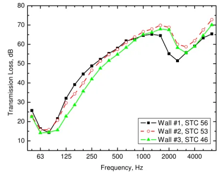
The main listening tests were carried out using three different wall constructions. The details of the 3 walls are given in Table 1 below. The first wall was a lightweight steel stud construction with 2 layers of 16 mm gypsum board on each face. There was 90 mm thick mineral fibre insulation in the cavity and the wall had an STC rating of 56. Figure 1 plots sound transmission loss (TL) versus frequency for all three walls.

The second wall was a wood stud wall with a single layer of 13 mm gypsum board on one face and two layers of 13 mm gypsum board on the other face, and which were mounted on resilient channels. There was 90 mm thick glass fibre insulation in the cavity and the wall had an STC rating of 53.

Wall number Face #1 Gypsum board Stud type Cavity insulation RC Face #2 Gypsum board STC #1 2 x 16 mm 92 mm Steel 90 mm mineral fibre No 2 x 16 mm 56 #2 13 mm 90 mm wood 90 mm glass fibre Yes 2 x 13 mm 53 #3 13 mm 90 mm wood 90 mm glass fibre Yes 13 mm 46

Table 1. Construction details of the 3 walls used in the main tests, (RC, resilient channels, STC Sound Transmission Class).

The third wall was a wood stud wall with a single layer of 13 mm gypsum board on one face and a single layer of 13 mm gypsum board on the other face, which was mounted on

resilient channels. There was 90 mm of glass fibre insulation in the cavity and the wall had an STC rating of 46. 63 125 250 500 1000 2000 4000 10 20 30 40 50 60 70 80 Tran sm ission Loss, dB Frequency, Hz Wall #1, STC 56 Wall #2, STC 53 Wall #3, STC 46

Figure 1. Measured sound transmission loss versus 1/3 octave band frequency for the 3 test walls.

2.3 Additional test wall constructions for k value evaluations

Two additional walls were constructed and tested. They were used only in evaluation of k values (see Section 5) over an extended range of conditions and were not used in any of the listening tests. Both walls were constructed with lightweight steel studs and included a single layer of 16 mm gypsum board on each face. Wall #4 was a double stud wall with glass fibre in both stud cavities and wall #5 was a single stud construction with glass fibre in the stud cavities. They had STC ratings of 66 and 57 respectively. Their descriptions are summarized in Table 2 and Figure 2 plots their sound transmission loss values versus frequency. Wall number Face #1 Gypsum board Stud type Cavity insulation RC Face #2 Gypsum board STC #4 16 mm Double 92 mm Steel Double 90 mm mineral fibre No 16 mm 66 #5 16 mm 92 mm steel 90 mm glass fibre No 16 mm 57

Table 2. Construction details of the 2 additional walls used to determine k values over an extended range. (RC, resilient channels, STC Sound Transmission Class).

63 125 250 500 1000 2000 4000 10 20 30 40 50 60 70 80 90 100 Tran sm ission Loss, dB Frequency, Hz Wall #4, STC 66 Wall #5, STC 57

Figure 2. Measured sound transmission loss versus 1/3 octave band frequency for the 2 additional test walls.

3. Subjective Test Procedure

The listening tests were intended to validate earlier listening tests [1,4] that included a wide range of speech and noise levels but that were carried out in simulated conditions without any reflected sounds. In the previous tests, the modification of the spectrum of speech sounds due to propagation though walls was simulated by appropriate

equalization of the speech and presented in combination with various noise sounds. The simulated transmitted speech sounds were presented to subjects over a loudspeaker system in front of them and ambient noises were reproduced by another loudspeaker system above them. The acoustical environment of the listening test room was very dead so that listeners heard only the direct sound from the loudspeakers. These previous tests were also carried out in a more carefully controlled manner than was possible with the current tests and they also involved a more rigorous process for selecting subjects. However, the new tests were only intended to determine whether similar results could be found in more realistic conditions.

3.1 Speech and noise levels

In the new validation tests, the recorded test sentences were reproduced using a

dodecahedron loudspeaker located approximately 2 m from the centre of the test wall in the large reverberation chamber. The speech sounds were naturally transmitted through the test wall into the small chamber where the listener was located. Foam sound

absorbing material was added to both reverberation chambers to reduce the reverberation times (averaged over frequencies from 160-5k Hz) in the small chamber to 0.64 s and in the large chamber to 0.80 s. The measured reverberation times with the added sound absorbing material are plotted versus 1/3 octave band frequency in Figure 3. With the added sound absorbing material present, the listeners heard speech sounds in realistic conditions representative of real rooms and heard speech sounds that had been transmitted through real walls.

125 250 500 1000 2000 4000 0.0 0.5 1.0 1.5 2.0 Reve rb erat io n time , s Frequency, Hz RT small RT large

Figure 3. Measured reverberation times in the reverberation chambers with the added sound absorption present during the listening tests.

The test sentences were assembled and edited as wav files using the Cool Edit Pro sound editing software. The integrated 1/3 octave band spectrum of each test sentence was measured directly at one microphone position in the large reverberation chamber about

2 m from the loudspeaker source. By using a pink noise signal reproduced by the same omni-directional loudspeaker and measured at the same microphone position as well as at the 9 standard microphone positions used in this reverberation chamber, it was possible to convert the measured speech levels to the levels that would have been measured at the 9 standard microphone positions and to calculate a room average source room speech level. Next the attenuations of a white noise signal, from the room average levels in the source room (measured at the 9 standard microphone positions) to positions 0.25 m from the test wall in the small chamber were measured. The transmitted levels were measured for an array of 15 positions in the central portion of the test wall and with each position 0.25 m from the wall surface. Using these 1/3 octave band attenuations and the source room average speech levels, the received speech levels were determined, in 1/3 octave bands, for each test sentence.

Ambient noise was added to the small reverberation chamber from a single loudspeaker located across the room from the listener. A pink noise wav file from Cool Edit Pro was further equalized to have an approximately –5 dB/octave spectrum shape. The ambient noise levels were measured using a single microphone at the location of the listener’s head. Three different ambient noise levels were used: 24, 29 and 34 dBA.

From the received speech levels and the ambient noise levels, it was possible to calculate various signal-to-noise ratio measures indicative of the degree of speech security at the position of the listener’s head (See Appendix 3 for equations). For example, the uniform weighted signal-to-noise ratio measure SNRUNI32 has been shown to relate well to

subjective judgments of the thresholds of cadence audibility and intelligibility of speech [1,4]. Received speech levels and ambient noise levels were adjusted to give a range of

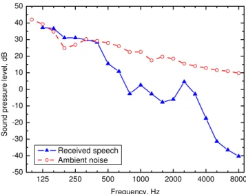
SNRUNI32 values expected to correspond to conditions varying from speech being inaudible to most listeners, to speech being somewhat intelligible to most listeners. Figure 4 illustrates an example of one transmitted speech spectrum and the corresponding ambient noise spectrum at the position of the listener’s head. The SNRUNI32 value for these data is –16.0 dB. 125 250 500 1000 2000 4000 8000 -50 -40 -30 -20 -10 0 10 20 30 40 50 Soun d pr es sur e lev e l, d B Frequency, Hz Received speech Ambient noise

Figure 4. Example of received speech spectrum and ambient noise spectrum at the listener position. The combination has an SNRUNI32 value of –16.0 dB.

For each of the three test walls speech and noise levels were adjusted to give the most useful range of SNRUNI32 values. The intention was that the SNRUNI32 values should be evenly distributed over conditions from, not audible to most listeners, to quite intelligible to most listeners. This required range can be determined from the previous work that established relationships between the perceived thresholds and SNRUNI32 values and these previously derived relationships are included in Figure 5. On these curves the point where 50% of listeners found the sounds just audible or just intelligible is said to be the just noticeable threshold for that particular response. The just noticeable threshold of

audibility is seen to correspond to a SNRUNI32 value of –22 dB on Figure 5. Similarly the just noticeable threshold of cadence corresponds to a SNRUNI32 value of –20 dB and the just noticeable threshold of intelligibility to an SNRUNI32 value of –16 dB.

-30 -25 -20 -15 -10 -5 0 0.0 0.2 0.4 0.6 0.8 1.0 Fr act ion ab ove th reshold SNR_UNI32, dB Intelligibility Cadence Audibility

Figure 5. Fraction of listeners (a) understanding at least one word, (Intelligibility), (b) hearing the cadence of the speech, (Cadence) and (c) hearing any speech sounds

at all (Audibility), versus SNRUNI32 value [1,4].

The actual distribution of SNRUNI32 values for the tests of all three walls are illustrated in Figure 6. The SNRUNI32 values are seen to be evenly distributed from just below a value of –25 dB to a maximum of about –3 dB. -30 -25 -20 -15 -10 -5 0 0 1 2 3 4 5 N u mber of cases SNR_UNI32, dB

3.2 Listening Tests

The listening tests used the Harvard sentences [6] as the speech test material. Five examples of these sentences are included in Table 3. They are phonetically balanced and low predictability sentences. The recordings used were high quality 16 bit digital

recordings spoken by a male talker as used in our earlier listening tests in simulated conditions [1,4]. The test protocol consisted of first turning on the noise signal and then a few seconds later playing one sentence. A few seconds after the end of the sentence, the noise stopped. The start and stop of the noise was marked by a chime sound so that subjects did not miss the start of the often very low levels of noise. In a few cases there was no sentence present to minimize the probability of subjects always guessing that they did hear some speech.

After the noise had stopped, the subject told the experimenter what they had heard. They first said whether any speech sounds were audible, and then said if they could hear the cadence or rhythm of the speech. Then they repeated the parts of the sentence that they had understood back to the experimenter. The listener spoke to the experimenter, who was outside the test chamber, using a microphone.

Before starting the test, the experimenter explained the test procedure to each listener with some examples of test sentences and noise. The subjects then started with a practice test consisting of 10 sentences that included SNRUNI32 values distributed over the

complete range shown in Figure 6 so that they could experience the full range of possible test sentences. Table 3 shows a portion of the score sheet used. The complete tests

consisted of either 30 test sentences (walls #1 and #2) or 40 sentences (wall #3).

After all subjects had listened to all sentences it was possible to calculate the fraction of the subjects for each test sentence, who were able to hear any speech sounds, and

determine an estimate of the audibility threshold. Similarly from the number of subjects, who were able to hear the cadence of the speech, an estimate of the threshold of the cadence threshold was determined. The intelligibility threshold was determined from the fraction of the listeners who could understand at least one word of each test sentence. Finally, the number of the words understood for each sentence was used to determine the speech intelligibility score as the fraction correct.

Not No Heard Full

Sentence Audible Cadence Cadence Score

01 A king ruled the state in the early days. / 9 02 The ship was torn apart on the sharp reef. / 9

03 Sickness kept him home the third week. / 7

04 The wide road shimmered in the hot sun. / 8

05 The lazy cow lay in the cool grass. / 8

Table 3. Sample of score sheet for the threshold test.

Subjects were all unpaid volunteers who were employees of one of the three

organizations funding this work. (Public Works and Government Services Canada, Royal Canadian Mounted Police, and the National Research Council). Since the tests were quite short, it was not thought to be practical to test every listener’s hearing. In some analyses, better listeners were selected by including only the listeners with the 10 highest speech intelligibility scores on each test.

4. Subjective Evaluation Results

As described in the previous section, 4 types of scores were obtained. These were: (a) the fraction of subjects indicating speech sounds were audible (audibility threshold), (b) the fraction of listeners indicating that they heard the cadence of the speech (cadence

threshold), (c) the fraction of the listeners that understood at least one word (intelligibility threshold), and (d) the speech intelligibility scores.

These scores were first plotted versus signal-to-noise ratio measures separately for each wall test. However, it was not possible to detect systematic differences among the results for the different walls and the data for all three wall tests were combined. Because no screening of subjects for hearing sensitivity was possible, some may have had some hearing loss. Therefore, the data were analysed first for all subjects and a second time for the best 10 listeners on each test (in terms of intelligibility scores). The best 10 listeners were expected to exclude listeners with less sensitive hearing or others who may have not been sufficiently fluent in English. The results for the 10 best listeners are included in this section. The data for all listeners are included in Appendix 1.

4.1 Audibility thresholds

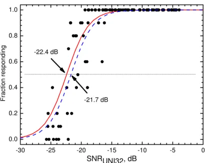
Figure 7 plots the fraction of listeners indicating that they heard some speech sounds versus SNRUNI32 values for the combined data from the tests of all three walls. Each point indicates the fraction of the 10 best listeners that heard speech sound for that particular condition. The solid line in this plot is the best-fit regression line obtained in the previous work [1,4]. The dashed line is the same form of curve but shifted to the right to better fit the new measured data. (The equations of the best-fit lines and regression coefficients are included in Appendix 1 in Tables A1.1 and A1.2). The amount of shift to the right was that which minimized the RMS error between the measured scores and the new best-fit line. In Figure 7, the shift is only 0.7 dB (i.e. –22.4 dB to –21.7 dB at the just noticeable audibility threshold). Given the large amount of scatter in the data, it is very unlikely that there is a significant difference between the new and previous best-fit lines.

To test the significance of the difference between the old results and the new results, one could calculate the standard deviation of the measured values about the new best-fit line in terms of SNRUNI32 values. Unfortunately this cannot be done for scores of either 0 or 1 for which it is not possible to define an SNRUNI32 value for this type of equation.

However, the standard deviation of the data points about the new best-fit line was calculated for all other points to give some indication of the relevance of the shift between the two best-fit lines. For the results in Figure 7, the standard deviation of the remaining data points (excluding points with scores of 0 or 1) about the new best-fit line was ±2.2 dB in terms of SNRUNI32 values. This is much larger than the 0.7 dB shift, and indicates that within the limits of the data, the new audibility data replicates and hence validates the previous results with respect to the audibility of transmitted speech sounds.

-30 -25 -20 -15 -10 -5 0 0.0 0.2 0.4 0.6 0.8 1.0 Fract ion respondi ng SNR_UNI32, dB -21.7 dB -22.4 dB

Figure 7. Fraction of listeners indicating that they heard some speech sounds for each test sentence from all three wall tests. Solid line is best-fit line from previous work [1,4]

and the dashed line is the new best-fit line to the current data. Horizontal dotted line indicates the threshold of audibility.

4.2 Cadence thresholds

The fractions of the best 10 subjects indicating that they heard the cadence of the speech sounds versus SNRUNI32 values are shown in Figure 8. For these data the new best-fit line is shifted 2.5 dB to the right (i.e. –20.0 to –17.5 dB) to minimize the vertical RMS deviations of the data about the line.

-30 -25 -20 -15 -10 -5 0 0.0 0.2 0.4 0.6 0.8 1.0 F racti on re spo n di n g SNR_UNI32, dB -20.05 dB -17.5 dB

Figure 8. Fraction of listeners indicating that they heard the cadence f the speech sounds for each test sentence from all three wall tests. Solid line is best-fit line from previous

work [1,4] and the dashed line is the new best-fit line to the current data. Horizontal dotted line indicates the threshold of cadence.

For these results the standard deviation of the data about the new best-fit line in terms of

SNRUNI32 values was ±1.6 dB. That is, the shift of the new best-fit line relative to the previous best-fit line is a little larger than the standard deviation of the data points about the best-fit line (excluding points with scores of 0 or 1). This suggests that in the new tests, for a given SNRUNI32 value, listeners were a little less likely to hear the cadence of the speech sounds than in the previous work. On average one would have to increase the

SNRUNI32 values for each test sentence by 2.5 dB to obtain the same results as in the previous experiments that used simulated conditions.

4.3 Intelligibility thresholds

Figure 9 plots the fraction of listeners who understood at least one word versus SNRUNI32 values. For these data the new best-fit line is shifted 4.9 dB to the right to minimize the vertical deviations of the data about the line. This is a quite large shift and almost all of the data points are to the right of the previous best-fit line (the solid line in this figure). The standard deviation of the data about the new best-fit line in terms of SNRUNI32 values was ±3.0 dB. The shift in the new best-fit line relative to the previous best-fit line is significantly larger than the scatter of the data about the new best-fit line. For this data, listeners were much less likely to understand at least one word for a given SNRUNI32 value than in the previous work. These results do not replicate the previous work. They indicate a greater degree of speech security for a given SNRUNI32 value than did the previous results. According to the new results, the just noticeable threshold of intelligibility corresponds to an SNRUNI32 value of –11 dB rather than the –16 dB value from the previous work. (The dotted regression line on Figure 9 will be discussed in Section 4.5)

-30 -25 -20 -15 -10 -5 0 0.0 0.2 0.4 0.6 0.8 1.0 Frac tion res ponding SNRUNI32, dB -10.7 dB -15.64 dB

Figure 9. Fraction of listeners indicating that they understood at least one word in each test sentence from all three wall tests. Solid line is best-fit line from previous work [1,4]and the dashed line is the new best-fit line to the current data. Dotted regression

line is an approximate correction for reverberation effects. Horizontal dotted line indicates the threshold of intelligibility.

4.4 Speech intelligibility scores

The speech intelligibility scores are plotted versus values of the SNRSII22 weighted signal-to-noise ratio in Figure 10. (See Appendix 3 for definition of SNRSII22). They are plotted versus SNRSII22 values because this measure was shown to be better related to speech intelligibility scores than the SNRUNI32 measure. However, the results are quite similar to those for the speech intelligibility threshold in Figure 9, in that a quite large shift is required to align the new best-fit regression line with the measured speech intelligibility scores. In this case the new best-fit line is shifted 5.8 dB to the right relative to the previous best-fit line shown on Figure 10. The standard deviation about the new best-fit line in Figure 10 in terms of SNRSII22 values was ±2.9 dB. (The dotted regression line on Figure 10 will be discussed in Section 4.5)

Again the new results cannot be said to replicate the old results. The new data indicates much lower speech intelligibility scores at a given SNRSII22 value.

-30 -25 -20 -15 -10 -5 0 0.0 0.2 0.4 0.6 0.8 1.0 In telligibility score , fr action cor rect SNR_SII22, dB -12.91 dB -7.1 dB

Figure 10. Speech intelligibility scores for each sentence from all three wall tests. Solid line is best-fit line from previous work [1,4] and the dashed line is the new best-fit line to

the current data. The dotted regression line is an approximate correction for reverberation effects.

4.5 Discussion of Subjective Results

The main purpose of the listening test was to validate the previous subjective studies that were carried out in a carefully controlled manner using a wide range of simulated

conditions. The new results presented here do partially validate the previous results, but also indicate some significant differences. In particular, the mean trends for the threshold of intelligibility scores and for the speech intelligibility scores indicate differences of 5 to 6 dB relative to the previous studies. These are large and important differences that could lead to requiring walls with STC values 5 or 6 points larger than necessary. Such a large

difference could constitute a significant additional construction cost and it is essential to determine the cause of these differences.

On the other hand there are not significant differences between the audibility threshold results for the previous work compared to the new results presented here. These new results do validate the previous threshold of audibility of speech sounds and the just noticeable threshold of audibility of speech sounds corresponds to an SNRUNI32 value of -22 dB.

There was a little larger difference between old and new results for the threshold of cadence. The new best-fit line for the Top 10 subjects of the new results is shifted by 2.5 dB relative to the previous work.

There are many possible sources of error that could influence the results. For example there could be errors in the measurement of speech and noise levels. However, this is unlikely to be the cause of the differences, since the same measurements were used to calculate signal-to-noise ratios for audibility threshold scores and for intelligibility

threshold scores. Since there is good agreement for the threshold of audibility results, it is reasonable to assume that the speech and noise level measurements were correct in both studies.

It is more likely that the differences are due to factors that would affect the understanding of speech and not the simple perception of the presence of sound as in the audibility test. Perhaps the most obvious factor is reverberation. It is well known that the intelligibility of speech is influenced by both the signal-to-noise ratio and the reverberation time of the listening space. However, the effects of reverberation on speech intelligibility at the very low signal-to-noise ratios, that are of concern in speech security issues, are not well defined. In our experiments, the subjects listened to just audible speech modified by the reverberation of both the source and the receiving rooms, but no measure of the effects of reverberation was included.

It is possible to estimate the combined effects of signal-to-noise and reverberation by calculating useful-to-detrimental sound ratios. This will only be approximate because this measure has not been validated for low signal-to-noise ratio situations.

Useful-to-detrimental sound ratios are based on the knowledge that the direct speech sound and early arriving reflections of the speech sound are ‘useful’ to intelligibility and later

arriving speech sounds and ambient noise are ‘detrimental’ to speech intelligibility. When early arriving reflections are those arriving within 50 ms of the direct sound, the useful-to-detrimental ratio U50 is defined as follows [7],

dB , log 10 50 ⎭ ⎬ ⎫ ⎩ ⎨ ⎧ + = n ls es E E E U (1)

where, Ees is the direct and early-arriving speech sound energy over the first 50 ms

Els is the late arriving speech sound energy

En is the ambient noise energy.

Values of U50 can be calculated from the speech and noise levels at the listener’s position

from impulse response measurements or can be estimated from measured reverberation times and by assuming ideal exponential decays. In this case the C50 values have been

estimated from the measured reverberation times.

The linear early-to-late ratio is calculated from the reverberation time as follows.

(2)

1

/

L

=

e

−

E

where, T is the reverberation time. and C50 in decibels is,

(3)

{

}

U50 is then calculated as follows,

dB , / ) 1 / ( 1 / log 10 50 50 50 ⎭ ⎬ ⎫ ⎩ ⎨ ⎧ ⋅ + + = S N L E L E U (4)

where, N and S are the measured noise and speech levels at the listener respectively. For very small reverberation times, U50 values reduce to signal-to-noise ratios. To estimate the added effects of reverberation time, U50 values were calculated for all 100 conditions in the 3 listening tests and for two different reverberation times. One was a negligibly short value of 0.01 s and the other was derived from the measured

reverberation times in the two rooms during the tests. The latter were calculated by taking the square root of the sum of the squares of the reverberation times in the two rooms at each frequency. (This assumes that the reverberation effects of the two rooms would combine as two series resonant circuits). This resulted in an average reverberation time of 1.0 s over the frequencies from 160 to 5k Hz.

The average difference in U50 values over all 100 test conditions was 2.98 dB. That is, we would expect the effects of added reverberation to shift the original regression equations, obtained in the previous lab studies [1,4], to the right by about 3 dB. Such shifted

regression equations were calculated and are included as the dotted regression lines on Figures 9 and 10 for intelligibility threshold and intelligibility score results. These regression lines do not fit the data perfectly, but do represent a considerable

improvement. One could argue that these shifted regression lines do fit the trends of the better listeners or that some other factor(s) also influence the results. Either or both are quite possible.

One other possible contributing factor is the differences in the spatial characteristics of the sound fields to which the listeners were exposed. It is known that our ability to understand speech in noise is related to the spatial relationship of the speech and noise sources [8]. When the speech and noise sources are close together, it is more difficult to understand speech at a given signal-to-noise ratio than when the two sources are

separated. For the same signal-to-noise ratio, separating the speech and noise source leads to increased speech intelligibility scores. Unfortunately, most previous studies of these effects have been in simple conditions such as the free fields that exist in anechoic rooms and not in the more complex sound fields that are found in real rooms.

There were differences in the spatial characteristics of the sound fields that the subjects experienced in the two experiments. In the previous work [1,4], subjects listened in an acoustically dead space (close to free field conditions). The speech sounds arrived from a loudspeaker system directly in front of the seated subject and the noise sounds arrived from another loudspeaker system directly overhead. No reflected sound was introduced into the simulated sounds and the test room itself would have added only very minor amounts of reflected sound due to the highly sound absorbing material on the walls, the highly absorbing ceiling tiles and the carpet on the floor of the room. Such conditions would be expected to maximize a listener’s ability to understand speech.

In the current tests, speech sounds were radiated into one room with an average speech frequency reverberation time of 0.80 s (i.e. averaged over the frequencies 160 to 5k Hz); they travelled through a real wall and from the wall a further 0.25 m to the listener’s ear. Other speech sounds would reflect about the rooms and arrive a little later at the listener’s ears. The noise source was located to the opposite side of the listener and hence the direct speech and noise sounds were spatially separated. However, the noise source was in a room with a speech frequency average reverberation time of 0.64 s and the listener would hear reflected noise sounds from many directions.

Although the conditions in the current experiments were more realistic and more representative of listening in real rooms, it is not known how the subtle differences in added reflected speech and noise sounds would affect speech intelligibility scores. Small amounts of reverberant sound do not usually have large effects on the intelligibility of speech. However, it is possible we are more sensitive to the negative effects of

reverberation for the very low signal-to-noise conditions in these experiments. Our knowledge of the effects of the spatial separation of speech and noise sources is almost entirely based on the perception of only the direct sounds in free field conditions [8]. It is quite possible that the addition of reflected sound to the speech and noise signals

considerably modifies these effects.

These differences can only be resolved by some further subjective tests in which each of the possible contributing factors is systematically varied. However, the results of Figures 9 and 10 in show that to ignore these problems could lead to costly over design of the sound insulation by 5 STC points or more.

5. The Effect of the Receiving Space on Received Speech Levels

5.1 The need to experimentally evaluate k values

The proposed new procedure for evaluating the speech security of meeting rooms

involves measuring or predicting transmitted speech levels at points 0.25 m from the wall of the meeting room in some adjacent receiving space. The levels 0.25 m from the wall in the receiving space are given by the following expression,

L0.25 = LS - TL + k, dB (5)

where, LS is the average source room level, dB TL is the transmission loss of the wall, dB

k is to be empirically determined in these measurements, dB.

If the receiving space is an acoustical free field (e.g. outdoors), then Pierce [9] has shown theoretically that k should be approximately –3 dB. This same expression is used in a Japanese standard for sound transmission from indoors to outdoors and uses a k value of –3 dB [10]. However, Beranek [11] and a newer text by Irwin and Graf [12] both produce theoretical expressions that suggest that k should have a value of –6 dB when the

receiving space approximates conditions of an acoustical free field. Initial tests indicated that for measurements at 0.25 m from the test wall in real rooms, the value of k is closer to 0 dB and was modified a small amount by the properties of the receiving space. The purpose of the measurements reported here was to experimentally determine appropriate values of k for use in assessing the speech security of meeting rooms and so that L0.25 values can be accurately predicted for all conditions.

A standard sound transmission loss test (ASTM E90 [5]) of each wall was first carried out to determine the TL values. Mean source room sound levels, LS, and transmitted levels, L0.25, at positions 0.25 m from the test wall were measured in the receiving space for 4 different sound absorptive treatments of each of the two test rooms. Equation (5) was used to determine values of k for various amounts of sound absorption in both the source and receiving rooms for all 3 test walls. Adding various amounts of sound

absorbing foam material made it possible to vary the reverberation times in both rooms. Figure 11 shows four sets of reverberation times for each room varying from no added material (0%), to all of the available material added (100%). This figure shows that in both rooms large variations in reverberation time were obtained.

As the receiving room becomes more reverberant, the sound levels at points 0.25 m from the test wall will be increasingly influenced by the level of reverberant sound in the room. Accordingly, it is necessary to determine the reverberant sound level in each room and for each absorptive treatment to relate changes in k values to the changing reverberant sound levels. For an ideal diffuse sound field, the total sound level throughout the room is given by, dB , 4 4 log 10 ₂ ⎭ ⎬ ⎫ ⎩ ⎨ ⎧ ₊ + = A r Q L L _W π (6)

Q is the directivity factor for the source and Q =1 for an omni-directional source, r is the source-receiver distance, m,

A is the total sound absorption in the room, m2, and, from the Sabine reverberation time equation,

A = 0.161 V/T

where V is the room volume m3, and

T is the reverberation time in the room in s.

In equation (6) above, the first term in the curly brackets is related to the direct sound level and the second term gives the reverberant sound level. Therefore, we can calculate the reverberant level, Lrv, as proportional to 10 log[ 4/A ]. That is, we expect the

influence of the reverberant sound levels in the receiving space on the k values to be related to 10 log[ 4/A ].

125 250 500 1000 2000 4000 0 1 2 3 4 Rev e rb er at io n t im e , s Frequency, Hz Large Chamber RT 0% RT25% RT50% RT100% 0 1 2 3 4 5 Small Chamber RT 0% RT25% RT50% RT100% Rev e rberat ion t ime, s

Figure 11. Measured reverberation times in each test chamber for each of the 4 absorptive treatments varying from no added absorption (0%) to the addition of all of the

5.2 Measurement results for the 3 main test walls

Since each of the quantities TL, LS, and L0.25, varies with frequency, averages over the frequency range of interest for speech (160 - 5k Hz) were determined. Using equation (5) and these frequency-averaged values of TL, LS, and L0.25, k values were determined for the 4 absorptive treatments for all 3 test walls. For the variations of the amount of absorption in the receiving space this resulted in 12 different estimates of k. These are plotted versus 10 log{4/A} (which is proportional to the reverberant sound level) in Figure 12. -10 -8 -6 -4 --2 -1 0 1 2 3 2 Wall #1 Wall #2 Wall #3 k , dB 10 log{4/A}, dB k = 0.423 L_RV +3.133

Figure 12. Experimentally determined k values versus 10 log{4/A} for averages over the frequency range from 160 to 5k Hz.

In Figure 12, there is a highly significant relationship between k values and 10 log{4/A}. The trend is similar for all 3 test walls and the mean trend is given by the following equation,

k = 0.432 {10 log[4/A]} + 3.133, dB (7)

Substituting this expression for k into equation (5) gives,

L0.25 = LS – TL + 4.23*log(4/A) + 1.325, dB (160-5k Hz) (8)

The effects of variations of the amount of sound absorption in the source room were also investigated. Although there were very small effects, they were not statistically

significant and not of practical importance. The results of these tests are given in Appendix 2.

Using the k values predicted by equation (7), measured and predicted levels 0.25 m from the test wall in the receiving space, L0.25, were compared as a function of frequency for each of the test walls. These comparisons are shown in Figure 13. Even though the k value is based on an average over frequencies (and over the results from 3 walls), there is excellent agreement between measured and predicted values at all frequencies.

125 250 500 1000 2000 4000 20 30 40 50 60 70 Wall #3 STC 46 L0. 25 , d B Frequency, Hz 20 30 40 50 60 70 Wall #2 STC 53 L0. 25 , d B 20 30 40 50 60 70 80 Measured Predicted L0. 25 , d B Wall #1 STC 56

Figure 13. Comparison of measured and predicted transmitted sound levels, L0.25, versus 1/3 octave band frequency for each of the three test walls.

5.3 Extended results for k values using tests of 2 additional walls

The results in Figure 12 show a simple linear relationship between the experimentally determined k values and the 10 log{4/A} values. However, Pierce’s theoretical work suggests that k should be –3 dB for propagation into a space that is a free field. This would suggest that for very low reverberant sound levels (i.e. 10 log{4/A} values) the values of k should asymptotically approach –3 dB and the linear trend in Figure 12 should not continue at very low 10 log{4/A} values.

To attempt to confirm this expectation and to extend the results to a wider range of conditions, tests on two additional walls were carried out. The two additional walls were constructed and sound transmission measurements to points 0.25 m from the wall in the receiving space were made for a wider range of absorptive treatments to the receiving room. The walls are described in Section 2.3 and had STC values of 57 and 66. The conditions in the receiving room varied from no treatment to the most absorption that could be added to the room. The measured reverberation times for these conditions averaged over the frequencies from 160 to 5k Hz varied form 0.3 to 3.3 s. Further details are included in Appendix 2.

To maximize the available data, the results of the main test of the first 3 walls were combined with those of the extra 2 walls. During the listening tests (using the first three

walls) the source room also included absorption to create more realistic listening

conditions for those tests. During the tests of the extra 2 walls, all absorbing material was used only in the receiving room. As described in Appendix 2, a correction was made for the small difference cause by the different conditions in the source room based on

measurements of varied absorption in the source room. This approach made it possible to include a much larger range of absorptive treatments in the receiving space and hence a wider range of 10 log{4/A} values.

The relationship between k values and the reverberant sound level (10 log(4/A)) for the combined data of all 5 wall tests is plotted in Figure 14. The tests of the extended conditions led to a wider range of reverberant levels compared to the main tests of the 3 walls used in the listening tests shown in Figure 12. The combined data in Figure 14 seem to closely follow a smooth monotonic relationship with only a small amount of scatter. The best-fit 2nd order polynomial regression line is shown on Figure 14 and is given by the following equation.

k = 0.023{10 log[4/A]}2 + 0.717{10 log[4/A]} + 3.963, dB (9) The RMS error about the regression line is only ±0.19 dB. That is, most of the time one would expect to be able to predict the k value for some situation from the related

reverberant level within an error of only ±0.19 dB.

It is clear that the results in Figure 14 make it possible to accurately predict k values for conditions of specified amounts of reverberation and from the corresponding reverberant sound level. However the conditions included in this graph represent a broader range than is likely to occur in typical meeting rooms. The two rectangular boxes were added to indicate the range of conditions likely for a typical smaller or larger meeting room as the receiving space. -14 -12 -10 -8 -6 -4 -2 -2 -1 0 1 2 3 k, dB 10log{4/A}, dB y = 0.023x2 + 0.717x + 3.963 R2 = 0.974 RMS error = 0.19 dB Small room Large room

Figure 14. Experimentally determined k values versus 10 log{4/A} for averages over the frequency range from 160 to 5k Hz for the data from all 5 wall tests.

The smaller room was assumed to have a volume of 150 m3 with likely reverberation times varying from 0.3 to 1.2 s. The larger room was assumed to have a volume of 500 m3 and with reverberation times varying from 0.5 to 1.6 s. Most smaller rooms would have much smaller reverberation times than 1.2 s and the range of likely conditions is probably smaller than the possible ranges indicated by the boxes in Figure 14.

Although one could accurately predict particular k values from the regression line of Figure 14, one could also get a reasonably close k value from an estimate of the room reverberation time and size and a quick visual check of Figure 14. The likely range of k values for most typical meeting rooms is really quite small (i.e. –1 ±0.5 dB).

Although from theoretical considerations k is expected to approach –3 dB for very low reverberant sound levels, this does not seem to occur in real rooms. The data in Figure 14 suggest that even extrapolating to lower reverberant levels would not lead to k values much less than –1.5 dB.

6. Conclusions

This report gives the results of two types of validation tests. The first type were listening tests to validate previous results from simulated conditions in the laboratory but in which the new tests were carried out in more realistic listening conditions. The second type of experiment was intended to validate a procedure for predicting transmitted speech levels at points 0.25 m from the outside of a meeting room.

6.1 Listening tests

The listening tests measured subject’s ability to hear and understand speech sounds from an adjacent meeting room.

• A listener’s ability to detect the audibility of speech sounds and the resulting

estimate of the threshold of audibility agreed quite well with the previous laboratory studies.

• Their ability to detect the cadence of the speech sound and the resulting estimate of the threshold of cadence were a little different than in the previous laboratory experiments.

• A subject’s ability to understand speech and the threshold of the intelligibility of speech were quite different than in the previously published experiments. In the new experiments, that include speech transmission through actual walls and room reverberation, listeners found it more difficult to understand speech than in the previous experiments at the same signal-to-noise ratios. The differences were of the order of 5 dB or more and hence are of considerable practical importance.

Estimates of the additional effect of reverberation on the new results could explain about 3 dB of this difference. Room reverberation may also make it more difficult to detect the cadence of speech sounds for these situations with low signal-to-noise ratios. It is

probable that the different spatial relationships of the noise and speech sources relative to the listeners in these tests also influence the new results. Although such effects have been reported in simple experiments in anechoic rooms, it is not possible estimate their likely magnitude for the more realistic conditions of the new results.

It is also possible that the less critical procedures for selecting subjects influenced the differences. Because the audibility results were approximately the same as in the

previous experiments, this may indicate that the Top 10 listeners in the new experiments had, on average, hearing sensitivities equal to the previous group. It is possible that the new listener group were a little less fluent in English than the previous subjects. It is important to investigate the effects of room reverberation and the spatial properties of the sounds arriving at the listeners in more detail because they would appear to have a major effect on a listener’s ability to understand speech in conditions of low signal-to-noise. Ignoring these effects could lead to costly over-design of the speech security of meeting rooms.

6.2 Predicting transmitted speech levels

The experiments to validate the procedure for predicting transmitted speech levels at points 0.25 m from the outside boundary of a meeting room indicate that this can be done

very accurately. The effect of the receiving room reverberation can be estimated within ±0.19 dB if reverberation times are known in the receiving room. Even without precise knowledge of the receiving room reverberation times, the effect of reverberation in the room will usually be no more than ±0.5 dB on the transmitted speech levels. Because the new procedure involves measurements close to the room boundary that is the source of the transmitted sound, the effects of receiving room reverberation are quite small as intended and could frequently be ignored.

Appendix 1. Subjective Test Results

Section 4 included a summary of the subjective ratings of intelligibility and audibility of speech sounds and of the cadence of the speech sounds. Results presented in Section 4 were for the best 10 listeners in each test. This appendix includes results for all listeners and compares them with the results for the best 10 listeners. It also includes details of the regression equations fitted to these data.

The equations fitted to the data were the sigmoidal shaped Boltzmann equation as was used in the previous work [1,4]. These curves have asymptotes to 0 for low x values and to 1 for high x values. This is ideal for the subjective ratings that vary from a possible low of 0 (e.g. not at all intelligible or audible) to a possible maximum of 1 (completely

intelligible or audible). The form of this equation is given below, in which F(x) would represent the subjective scores and x the signal-to-noise ratio measure,

⎟ ⎠ ⎞ ⎜ ⎝ ⎛ − + − = B A x x F exp 1 1 1 ) ( (A1.1)

Here A and B are parameters defining the offset and slope of the curve respectively. The curve has asymptotes of +1 at x = ∞ and 0 at x = –∞.

This appendix includes 4 pages each with two graphs. The upper graph is for all listeners. The lower graph is for the 10 best listeners (in terms of intelligibility scores) and repeats the information in Section 4 to make comparisons easier.

Table A1.1 gives the regression coefficients for the various best-fit lines illustrated in this report. Regression coefficients A and B are defined in equation A1.1. The column

labelled ‘JASA’ corresponds the previously published relationships [4]. The column labelled ‘Top 10’ is for the best 10 subjects and given by the dashed lines in Figures 7 to 10 in Section 4 and Figures A1.1b, A1.2b, A1.3b and A1.4b in this Appendix. The columns labelled ‘Shift’ indicate how many dB the new curves are shifted relative to the previous results (in the column labelled ‘JASA’). The table also gives the RMS

deviations of the scores about the various best-fit lines.

The threshold of audibility results in Figures A1.1a and A1.1b are very similar for the All subjects results and for the Top 10 subjects results. In Table A1.1 the shifts of the new best-fit curves compared to the previous results are almost the same (i.e. 0.7 dB for the Top 10 group and 1.0 dB for the All subject group). There were only very small differences in the abilities of the two subject groups to detect speech sounds.

For the threshold of cadence results in Figures A1.2a and A1.2b the differences between the two subject groups were only slightly larger. The corresponding results in Table A1.1 indicate a 3.2 dB shift for the new best-fit curve for the All subjects group compared to a 2.5 dB shift for the Top 10 subjects group. That is, the Top 10 subjects group were on average a little better at detecting the cadence of the speech than were the All subjects group.

The threshold of intelligibility results in Figures A1.3a and A1.3b indicate larger

differences between the results for the two groups of listeners. The results in Table A1.1 show that for the All subjects group, the new best-fit regression curve was shifted 7.6 dB

compared to only 4.9 dB for the Top 10 listener group. That is, the Top 10 group of listeners were considerably better at understanding speech than the All subjects group. The dotted regression lines on these two figures include the estimated additional effects of reverberation discussed in section 4.5.

The results for the intelligibility scores in Figures A1.4a and A1.4b and Table A1.2 indicate similar results to those for the threshold of intelligibility. The new best-fit curves were shifted more for the All subjects group than for the Top 10 subjects group to best fit each data set. Again the Top 10 listeners were on average better able to understand the speech test material than the average of the All listeners group. The dotted regression lines on these two figures include the estimated additional effects of reverberation discussed in section 4.5.

Value Audibility threshold

JASA Top 10 Shift All Shift

A -22.41 -21.7 0.7 -21.4 1.0 B 1.8053 1.8053 1.8053 RMS error 0.144 0.136 0.123 Cadence threshold A -20.05 -17.5 2.5 -16.8 3.2 B 1.4037 1.4037 1.4037 RMS error 0.214 0.124 0.123 Intelligibility threshold A -15.64 -10.7 4.9 -8.0 7.6 B 1.8379 1.8379 1.8379 RMS error 0.322 0.193 0.159

Table A1.1 Regression coefficients and RMS errors (deviations) about the various regression lines for fits to the scores of the fraction of listeners indicating hearing or

understanding of speech versus SNRUNI32 values.

Value Intelligibility score

JASA Top 10 Shift All Shift

A -12.91 -7.1 5.8 -6.0 6.9

B 2.1987 2.1987 2.1987

RMS

error 0.383 0.100 0.086

Table A1.2 Regression coefficients and RMS errors (deviations) about the regression lines for speech intelligibility score versus SNRSII22 values.

For comparisons with the results of the previous work it is better to use the results from the Top 10 group of listeners since the previous work included hearing sensitivity and a screening test to restrict the subjects to those with better hearing and who were more successful on this type of listening test. However, the Top 10 subjects in the current tests may still have been not as capable as those in the previous tests.

-30 -25 -20 -15 -10 -5 0 0.0 0.2 0.4 0.6 0.8 1.0 Fr action responding SNR_UNI32, dB -21.4 dB -22.4 dB

Figure A1.1a Fraction of All listeners indicating that they heard some speech sounds for each test sentence from all three wall tests. Solid line is best-fit line from previous work

[1,4] and the dashed line is the new best-fit line to the current data. Horizontal dotted line indicates threshold of audibility.

-30 -25 -20 -15 -10 -5 0 0.0 0.2 0.4 0.6 0.8 1.0 F raction r esp onding SNRUNI32, dB -21.7 dB -22.4 dB

Figure A1.1b Fraction of Top 10 listeners indicating that they heard some speech sounds for each test sentence from all three wall tests. Solid line is best-fit line from previous work [1,4 ] and the dashed line is the new best-fit line to the current data. Horizontal

-30 -25 -20 -15 -10 -5 0 0.0 0.2 0.4 0.6 0.8 1.0 F raction r esp onding SNR_UNI32, dB -20.05 dB -16.8 dB

Figure A1.2a Fraction of All listeners indicating that they heard the cadence of the speech sounds for each test sentence from all three wall tests. Solid line is best-fit line from previous work [1,4] and the dashed line is the new best-fit line to the current data.

Horizontal dotted line indicates threshold of cadence.

-30 -25 -20 -15 -10 -5 0 0.0 0.2 0.4 0.6 0.8 1.0 Fracti on re sp on di n g SNRUNI32, dB -20.05 dB -17.5 dB

Figure A1.2b Fraction of Top 10 listeners indicating that they heard the cadence of the speech sounds for each test sentence from all three wall tests. Solid line is best-fit line from previous work [1,4] and the dashed line is the new best-fit line to the current data.

-30 -25 -20 -15 -10 -5 0 0.0 0.2 0.4 0.6 0.8 1.0 Fractio n re spon di ng SNR_UNI32, dB -8.0 dB -15.64 dB

Figure A1.3a Fraction of All listeners who understood at least one word for each test sentence from all three wall tests. Solid line is best-fit line from previous work [1,4] and the dashed line is the new best-fit line to the current data. The dotted regression line is an

approximate correction for reverberation effects. Horizontal dotted line indicates threshold of intelligibility. -30 -25 -20 -15 -10 -5 0 0.0 0.2 0.4 0.6 0.8 1.0 Frac tion res ponding SNRUNI32, dB -10.7 dB -15.64 dB

Figure A1.3b Fraction of Top 10 listeners who understood at least one word for each test sentence from all three wall tests. Solid line is best-fit line from previous work [1,4] and the dashed line is the new best-fit line to the current data. The dotted regression line

is an approximate correction for reverberation effects. Horizontal dotted line indicates threshold of intelligibility.

-30 -25 -20 -15 -10 -5 0 0.0 0.2 0.4 0.6 0.8 1.0 Intell igi bil

ity score, fraction

correct

SNR_SII22, dB

-6.0 dB -12.91 dB

Figure A1.4a Mean speech intelligibility score of All listeners for each test sentence from all three wall tests. Solid line is best-fit line from previous work [1,4] and the dashed line is the new best-fit line to the current data. The dotted regression line is an approximate

correction for reverberation effects.

-30 -25 -20 -15 -10 -5 0 0.0 0.2 0.4 0.6 0.8 1.0 Intell igi bil

ity score, fraction

correct

SNR_SII22, dB

-12.91 dB

-7.1 dB

Figure A1.4b Mean speech intelligibility score of the Top10 listeners for each test sentence from all three wall tests. Solid line is best-fit line from previous work [1,4] and the dashed line is the new best-fit line to the current data. The dotted regression line is an

Appendix 2. Effects of the Receiving Space on Transmitted Speech

Levels

Figure 12 in Section 5 of the main report plotted k values versus 10 log(4/A) values for 10 log(4/A) values averaged over the frequencies normally associated with speech (i.e. 160 to 5k Hz). Similar results were also produced for averages over the 1/3 octave band frequency range from 100 to 5 kHz that is associated with most building acoustics measurements. These latter results may be useful where the focus is not strictly on speech. Figure A2.1 plots k values versus 10 log{4/A} (i.e. the reverberant level) for frequency averages of 10 log(4/A) values over the 1/3 octave band range from 100 to 5k Hz as well as for the frequency range from 160 to 5k Hz.

-10 -8 -6 -4 --2 -1 0 1 2 3 2 k = 0.479 {10 log(4/A)} +3.826 160-5k Hz 100-5k Hz k , dB 10 log{4/A}, dB k = 0.423 {10 log(4/A)} +3.133

Figure A2.1 Experimentally determined k values versus 10 log{4/A} for averages over two different frequency ranges: (a) from 160 to 5k Hz and (b) from 100 to 5k Hz.

In both cases there are highly significant relationships and with slightly different regression equations. The two best-fit regression equations are:

For 160 to 5k Hz, k = 0.423 {10 log(4/A} + 3.133 (A2.1)

For 100 to 5k Hz, k = 0.479 {10 log(4/A} + 3.826 (A2.2)

The effect of varied sound absorption in the source room was also evaluated. Again k values were calculated from measured TL, LS and L0.25 values as described in Section 5. The k values were calculated for averages over the two different frequency ranges (100 to 5k Hz and 160 to 5k Hz), for 4 different absorption treatments and for all 3 test walls. The results are given in Figure A2.2.

Although the graph does suggest systematic small increases in k values with increasing values of 10 log(4/A), the relationships are not statistically significant and therefore may be due to chance. They suggest changes in k values of up to about 0.5 dB over the full range of absorption treatments. It may be that when large amounts of absorption are added, the source room is not ideally diffuse and the measured room average levels

underestimate the actual levels incident on the test wall by up to about 0.5 dB. This would lead to slightly higher transmitted levels L0.25 and when these values are entered into equation (5) (in Section 5.1) to determine k values, they would be in increased by the same small amount. It therefore seems most likely that if the results in Figure A2.2 mean anything, they suggest small errors can occur when the source room is highly absorptive and does not have an approximately diffuse sound field.

-12 -10 -8 -6 -2 -1 0 1 2 3 160-5k Hz Wall #1 Wall #2 Wall #3 100-5k Hz Wall #1 Wall #2 Wall #3 k , dB 10 log{ 4/A}, dB

Figure A2.2 Experimentally determined k values versus 10 log{4/A} for variations of absorption in the source room. The solid lines are for averages over the frequency ranges

from 160 to 5k Hz and the dashed lines for the frequency range from 100 to 5k Hz.

As discussed in section 5.1, previous theoretical considerations [9] and a Japanese standard [10] suggest, that for free field conditions in the receiving space, k should

approximate –3 dB. The lowest k values on Figure A2.1 are about –1. It was assumed that if even more absorption had been added to the receiving room, conditions would

eventually approximate a free field and lower k values would be determined. Some further tests were therefore carried out to determine if k values would tend to approach a value of –3 dB in very highly absorptive receiving spaces.

Two additional walls (described in Section 2.3) were constructed and sound transmission measurements to points 0.25 m from the wall in the receiving space were made for a wider range of absorptive treatments to the receiving room. These varied from no treatment to the most absorption that could be added to the room. The measured reverberation times of these conditions of varied absorption are shown in Figure A2.3. The corresponding average reverberation times over speech frequencies (160 to 5k Hz) varied form 0.3 to 3.3 s.