HAL Id: hal-01205485
https://hal.archives-ouvertes.fr/hal-01205485v2
Submitted on 18 Jan 2017HAL is a multi-disciplinary open access
archive for the deposit and dissemination of sci-entific research documents, whether they are
pub-L’archive ouverte pluridisciplinaire HAL, est destinée au dépôt et à la diffusion de documents scientifiques de niveau recherche, publiés ou non,
Energy efficiency policies for space heating in EU
countries: A panel data analysis for the period
1990–2010.
Eoin Ó Broin, Jonas Nässén, Filip Johnsson
To cite this version:
Eoin Ó Broin, Jonas Nässén, Filip Johnsson. Energy efficiency policies for space heating in EU countries: A panel data analysis for the period 1990–2010.. Applied Energy, Elsevier, 2015, 150, pp.211-223. �10.1016/j.apenergy.2015.03.063�. �hal-01205485v2�
1 TITLE: 1 Energy efficiency policies for space heating in EU countries: A panel data analysis for the period 1990– 2 2010. 3 4 CORRESPONDING AUTHOR FAMILY NAME: 5 6 Ó Broina, 7 8 CORRESPONDING AUTHOR FIRST NAME: 9 10 Eoin 11 12 e‐mail: eoin.obroin@chalmers.se 13 Phone: +46317721450 14 Fax: +46317723592 15 16 CO –AUTHOR 1: 17 18 Jonas Nässénb 19 e‐mail: jonas.nassen@chalmers.se 20 21 CO‐AUTHOR 2: 22 23 Filip Johnssona 24 e‐mail: filip.johnsson@chalmers.se 25 26 aDepartment of Energy and Environment, 27 Energy Technology, 28 Chalmers University of Technology, 29 SE‐412 96 Göteborg 30 31 b Department of Energy and Environment, 32 Physical Resource Theory, 33 Chalmers University of Technology, 34 SE‐412 96 Göteborg
35
Energy efficiency policies for space heating in EU countries:
1A panel data analysis for the period 1990 to 2010.
2ABSTRACT
3We present an empirical analysis of the more than 250 space heating-focused energy efficiency policies 4
that have been in force at the EU and national levels in the period 1990–2010. This analysis looks at the 5
EU-14 residential sector (Pre-2004 EU-15, excluding Luxembourg) using a panel data regression analysis 6
on unit consumption of energy for space heating (kWh/m2/year). The policies are represented as a
7
regression variable using a semi-quantitative impact estimation obtained from the MURE Policy Database. 8
The impacts of the policies as a whole, and subdivided into financial, regulatory, and informative policies, 9
are examined. The correlation between the actual reductions in demand and the estimated impact of 10
regulatory policies is found to be stronger than the corresponding correlations with the respective impacts
11
of financial policies and informative polices. Together with the well-known market barriers to energy 12
efficiency that exist in the residential sector, these findings suggest that regulatory policy measures be 13
given a high priority in the design of an effective pathway towards the EU-wide goals for space heating 14
energy. 15
Keywords
16Residential; Econometrics; Efficiency; Policy; Space heat; Regulations
17
1
INTRODUCTION
18
Lowering the absolute energy demand of buildings is a key policy goal of the EU. This is to be achieved 19
mainly through improvements in end-use efficiency [1]. The indicative goal for Year 2020 is to lower 20
primary energy demand within the EU by 20% relative to a business-as-usual scenario. This goal is part of 21
the EU Climate and Energy Packet (known colloquially as the EU 202020 goal), and also includes the 22
mandatory goals that by Year 2020 there should be a 20% share for renewables in the energy supply and a 23
20% reduction in greenhouse gas emissions (relative to the levels in Year 1990) [2]. For the residential 24
sector, the energy savings target has been set at the higher level of 27% given the well-documented 25
savings opportunities that exist in this sector [3]. The multifaceted motivations behind the overall energy 26
savings goal include reducing dependence on fossil fuels imported from outside the EU, mitigating the 27
volatility associated with oil prices, increasing competitiveness by reducing energy costs, stimulating 28
employment in the construction sector, improving both the indoor and outdoor air quality via improved 29
ventilation and decreased emissions of combustion gasses, reducing noise pollution, and mitigating 30
climate change. However, studies have shown that the EU is on target to meet only half of its Year 2020 31
overall energy savings goal [4]. In addition, the negotiations surrounding the Energy Efficiency Directive 32
[5] have highlighted that it is not possible to lower EU Primary Energy Demand by more than 17% using 33
the measures agreed in the directive, meaning that a de facto 3% watering down of the savings through 34
efficiency target has occurred. 35
3
1 Nomenclature
CH Percentage of dwellings with Central Heating installed.
Delay1 Model A model used in this work in which the implementation of policies has been delayed by
1 year, to determine if there is a time lag in the impacts of efficiency policies that have been introduced.
EEW Energy Efficiency Watch Project
EP A time series variable constructed for the purpose of the present work to represent the residential sector heating-focused Efficiency Policies that are in place. EP is also subdivided into financial, informative and regulatory policies in this work.
EPBD EU Energy Performance of Buildings Directive
ESD EU Energy Services Directive
HAC Heteroskedasticity and Autocorrelation Consistent Standard Errors.
HDD Heating Degree Days.
High-, Medium- or Low-impact Policy A policy listed in the MURE Policy Database that is
estimated to reduce demand by >0.5%, 0.1%–0.5% or <0.1%, respectively.
Laspeyres Decomposition A method of index decomposition in which model variables are each in
turn changed to their final year (Year 2010) values, while the other model variables are kept at their base year (Year 1990) values. This allows the individual impact of a variable-on-demand to be estimated.
LSDV Least-Squares Dummy Variable-fixed effects panel data regression model.
MURE Policy Database An online database of all national and EU-wide sector-level efficiency
policies that have been introduced in the EU-28 countries and Norway since the 1970’s.
NEEAP National Energy Efficiency Action Plan
SQI Semi-quantitative impact. The name given to the ex post or ex ante evaluations of each of the policies in the MURE database. Policies are ranked as having a low, medium or high impact on the demand reduction in which they are found to or expected to result. These rankings are used in the present work to construct the EP, Financial, Informative and Regulatory policy variables.
Unit consumption of energy for space heating (kWh/m2/year) A time series variable
constructed for the purpose of this work that represents the sum of each energy carrier used for heating divided by total floor area. The unit is the square metre. Unit
consumption is an established indicator of energy efficiency progress, as it tracks changes in energy use related to efficiency improvement and is not influenced by changes in either population or dwelling size.
VIF Variance inflation factor. A statistical tool to detect the multicolinearity of a number of explanatory variables.
WAP Weighted Average Price. A time series variable constructed for the purpose of the present work that aggregates the prices of different energy carriers for heating into a single price weighted according to the proportion of each energy carrier in the heating mix.
Wald (F)Test A parametric statistical test used to examine the combined significance of a number of
explanatory variables.
Over the last decade, the European Commission has introduced a package of measures aimed at achieving 1
the Year 2020 goal of a 20% reduction in primary energy demand. These measures include the Energy 2
Performance of Buildings Directive (EPBD) [6], the Energy Services Directive [7], the Eco Design 3
Directive [8], and the Energy Labelling of Products Directive [9]. These are policy measures that seek to 4
drive technical innovation, the diffusion of efficient technologies, and the creation of a market for 5
efficiency. More recently, additional policies that aim to improve or enhance the aforementioned factors 6
have been introduced or debated, namely, the recast of the EPBD [10], the Energy Efficiency Directive 7
[11], and the proposed Energy Taxation Directive [12]. These EU directives are transposed into national 8
policy legislation by the respective countries and complement the energy savings measures that individual 9
countries have introduced to varying degrees since the 1970’s [13, 14]. 10
A study that looked at 30 years of experience in OECD countries with polices for increasing energy 11
efficiency [15] revealed that most Western European countries have undergone substantial energy 12
intensity reductions, distinct from structural changes, since 1973. These authors report that many policies 13
and programs have been adopted to increase energy efficiency, and some have clearly ‘‘made a 14
difference’’. The most influential policies have been energy codes, industrial voluntary agreements, 15
pricing initiatives, and financial incentives adopted at the national level, while EU-wide appliance 16
labelling and standards, and the new vehicle CO2 emissions intensity agreement also have had impacts.
17
However, they conclude that it is very difficult to estimate what fraction of the overall energy efficiency 18
improvement can be attributed to specific policy initiatives and what fraction is linked to other factors, 19
such as market forces and on-going technological change. 20
Although thorough descriptions of the efficiency policy options in existence and their theoretical bases in 21
terms of dealing with the well-known market barriers to efficiency are available in the literature [14, 16-22
23], most of these studies do not quantify ex post the effects of individual or portfolios of efficiency 23
policies. Gillingham and colleagues [18] have commented that most of the policy evaluation studies have 24
been ex ante, and while they are useful for understanding future policies, they do not demonstrate that a 25
policy has been effective. From a policymaker’s perspective and considering the well-known market 26
barriers to energy efficiency, it is of interest to know how well the existing and previous efficiency policy 27
frameworks have succeeded in reducing energy demand. Previous studies of this issue, which included 28
some ex post analyses, e.g., [24], have compared a projected baseline energy demand to the actual demand 29
outfall and postulated that the difference is due to policy-driven energy efficiency improvements and the 30
use of less-energy-intensive products. This approach is similar to the findings of indicator-based 31
efficiency evaluations [25]. Vine and co-workers [26] reported that the combination of mandatory 32
labelling which was introduced in the EU in 1992 and other efficiency policies improved the efficiency of 33
refrigeration appliances by 10% from 1992 to 1996. Hoicka et al. [27] showed that financial rewards can 34
increase both the levels of participation and outcomes in efficiency programmes. As part of the IPCC 4th
35
assessment (AR4) chapter on mitigation options for residential/commercial buildings, a qualitative 36
evaluation of 60 ex post efficiency case studies was carried out [28]. Appliance standards, building codes, 37
tax exemptions, and voluntary labelling were found to be the most effective policy instruments for 38
reducing demand. 39
5
Using a panel of 48 of the states in the USA, Horowitz [29] examined empirically whether states with 1
strong commitments to energy efficiency have lower levels of energy intensity than those with weak 2
commitments, and found that this was indeed the case. He also found that energy efficiency programmes 3
have a transformative effect on other macroeconomic variables, such as electricity price, income per 4
capita, and technological change, and that that there are spill-over efficiency effects from states with 5
strong commitments to efficiency towards states with weaker commitments. Filippini and colleagues [30] 6
also used panel data methodologies to examine empirically the impacts of energy policy instruments on 7
the estimated level of underlying energy efficiency in the EU residential sector, while Saussay et al. [31] 8
did the same for seven EU countries and Bigano et al. [32] did the same for all sectors. The two latter 9
studies [31 and 32] found that energy efficiency in the residential sector had been improved by the 10
application of, in particular, mandatory standards for buildings. Filippini et al. [30] found that financial 11
measures had the greatest impact, mandatory standards for appliances or buildings less of an impact; they 12
found no improvement in efficiency from informative policies. 13
These last three cited papers [30-32] represent a discourse initiated by Bigano et al. [32] in which panel 14
data econometric methods are used to examine the extents to which the energy efficiency-focused policies 15
introduced across the EU have succeeded in reducing energy demand. The three papers differ from more 16
common residential sector models in the literature, e.g. [16, 33], in that they explicitly include variables 17
that account for the introduction of energy efficiency policies. While all three papers provide valuable 18
insights into modelling methods and the impact of efficiency policies, the method that they use for 19
quantifying the actual efficiency policies in place is somewhat rudimentary. Bigano et al. [32] state in 20
their conclusions that: ‘It would be more interesting to use continuous instead of binary policy variables’, 21
while Saussay et al. [31] write that: ‘Finally, the parameterization we chose for the building energy codes 22
is admittedly fairly simple, and would call for further improvements’. Therefore, the present study 23
develops the aspect regarding the modelling of efficiency policy and as such presents a further 24
contribution to the discourse. Our focus is on the case of space heating energy demand in the EU-15 25
residential sector from 1990 to 2010. In addition, this paper describes other methodological developments, 26
which are outlined in the Methodology section and expands the literature review to place the work in a 27
broader perspective. In light of the methodological developments, the results obtained in the present work 28
reinforce the general findings of the previous studies [30-32] regarding the paramount importance of 29
regulatory policies as well as adding new results with regard to the impact of policy over time.This paper 30
is divided into four sections. Following the Introduction, Section 2 presents the approach used and then 31
describes the model parameters and the data used as inputs. This includes a description of the quantitative 32
method used in this work to represent energy efficiency policies applied to the residential sector. Section 3 33
presents results for the various models and a detailed discussion on the implications and interpretations of 34
the findings. Section 4 presents the conclusions drawn from the study. 35
2
METHODOLOGY
1This paper uses a panel data regression approach to estimate the energy savings conferred by the policy 2
portfolio in place across the EU1. In modelling terms, the core determinants of energy demand are defined
3
for the purposes of this paper as: energy price; personal income; the outdoor climate; the penetration of 4
central heating in the building stock; and a time trend, which is a linear approximation of other effects that 5
have occurred over the studied period. The latter include autonomous technical progress, fuel switching, 6
and structural changes. These explanatory variables are similar to those used by others [16, 37], except 7
that no alternative fuel price options, such as a response to an increase in the gas price, are employed. This 8
is because the dependent variable used in this study (space heating) is not substitutable. In considering 9
whether to employ a fixed or random effects panel data model to account for the unobserved heterogeneity 10
across a panel of countries, it has been argued [38] that a fixed effects model should be used. Their 11
argument is that the selection of countries for studies such as the one described in this paper is not 12
random, since the countries chosen are not exchangeable with other countries. Bigano et al [32] chose a 13
fixed effects rather than a random effects panel using the same justification. Dougherty [39] has explained 14
that if a panel is designed with OECD countries only, the countries are inherently not chosen randomly. 15
Dougherty [39] has also presented a model choice scheme, which for the purposes of this paper would 16
suggest the use of a fixed effects model. 17
In keeping with the previous studies [30-32], the present study incorporates an additional explanatory 18
variable that represents policies aimed at reducing energy demand via efficiency. The new variable is an 19
aggregation of relevant policies and measures introduced at the EU and national levels since the 1970’s 20
and is termed EP (Energy Policies) for the purposes of modelling. By introducing this variable, the 21
component of the time trend that otherwise would have represented efficiency policy is removed. As a 22
development, EP in the model is replaced by separate variables that represent different categories of 23
efficiency policies, to determine which particular policy categories have had the greatest impacts on 24
demand. For the purposes of the present work, the remaining determinants of energy demand, e.g., price, 25
income etc., are control variables, the coefficients of which are expected to concur with those reported in 26
the literature in terms of magnitude and polarity. 27
In the present work, the analysis is performed for energy demand for space heating in the residential 28
sector. The dependent variable used in this study is unit consumption (kWh/m2/year), as its temporal
29
dynamic is an established indicator of energy efficiency [25]. The period examined is 1990–2010. While 30
this interval is motivated primarily by the availability of the relevant data, it is also a historical period that 31
is of high relevance for policymakers who are designing contemporary efficiency policies. The work 32
carried out in [32] also used Unit Consumption as a dependant variable, while [30] looked at all energy 33
demand and [31] examined total space heating energy demand. 34
1
Various groups [34‐36] have presented comprehensive reviews of how panel data analysis can be used for energy demand studies.
7
Table 1 : Comparisons of the methodologies used in the present study and the previous studies [30‐32].
1
This paper Filippini et al. [30] Saussay et al.[31] Bigano et al. [32]
Temporal Scope 1990 – 2010 1996 – 2009 1990 – 2008 1980 ‐ 2006
Spatial Scope
EU‐15 except Luxembourg EU‐27 except Malta Seven EU countries: Austria, Denmark, Finland, France, Germany, Poland and the United Kingdom
EU‐15 plus Norway
Panel Structure Balanced Unbalanced Unbalanced Unbalanced
Panel approach Fixed Effects Fixed and Random Effects
separately Random Effects Fixed Effects Dependent variable Unit Consumption (kWh/m2/year) of residential sector space heating energy demand from five energy carriers: electricity, natural gas, oil, coal and district heating. Total energy demand in residential sector Sum of residential sector space heating energy demand from three energy carriers: electricity, natural gas and oil Unit Consumption for total energy demand in residential sector Price variable WAP for heat from five energy carriers coal, district heating, electricity natural gas and oil. Index of household energy prices WAP of market prices for three energy carriers: electricity, natural gas and oil. Electricity prices Policy Data Source
MURE Policy Database MURE Policy Database IEA BEEP Database MURE Policy Database
Policy parameterization Index that increases by 20, 10 or 1 every time a High‐, Medium‐, or Low‐impact policy is introduced respectively. Separate dummy variables for cases of 1–2 or ≥3 policies in a particular category that are in force. Index that increases by 1 for every year a policy is in force. Dummy variable for each year at least one policy in a particular category is in force. Inclusion of policy variables in model
Variable in panel OLS Stochastic Frontier Approach Stochastic Frontier Approach
Variable in panel OLS
Lagged effects of policy variables
Up to 7 years None Implicit via annually increasing policy index Up to 2 years Policy Categories Modelled Four: (i) All; (ii) Financial; (iii) Informative; and (iv) Regulatory Six: (i,ii) building standards; (iii,iv) financial; (v) appliances; and (vi) information
One: Building Standards Twelve: (i)Mandatory Standards for Buildings; (ii) Regulation for Heating Systems and hot water systems; (iii) Other Regulation in the Field of Buildings; (iv) Mandatory Standards for Electrical Appliances; (v) Legislative/Informative; (vi) Grants/subsidies; (vii) Loans/Others, (viii), Tax Exemption/Reduction; (ix) Tariffs; (x) Information/Education; (xi) Co‐operative Measures; (xii) Cross‐cutting with sector‐specific characteristics
Table 1 presents a comparison of the methodologies employed in the work presented in this paper and that 1
used in the previous studies [30-32]. In summary, the present paper encompasses methodological 2
advances that implement changes to: 1) the way that the policy data are interpreted (see Section 2.2); 2) 3
the time period used for the analysis; 3) how the time series of energy prices is calculated (see Section 4
2.3); 4) the process by which the econometric testing of model results is carried out (See Section 3.1); and 5
5) the dependant variable used (Unit Consumption for Space Heating). 6
2.1
Model description
7
The linear regression model of unit consumption for space heating, Iit, takes the form:
8
(1) 9
where Pit is a weighted average (by heating energy carrier for each individual country) real price of
10
energy, Yit is income per capita, CHit is the percentage of dwellings with central heating installed, HDDit
11
are heating degree days which are a proxy variable for the outdoor climate, t is a time trend, EPit is a
12
numerical representation of the energy efficiency policies in place, and εit is the residual term. The i and t
13
subscripts in Eq. (1) give the spatial and temporal parameters of the panel, respectively. Initially, other 14
choices of dependent variables for heating were tested, including the total heating demand (space heating 15
plus water heating plus heat for cooking), total per capita, and total per square metre. However, it was 16
decided to perform the work only for unit consumption for space heating for the EU-14 after taking into 17
consideration the following issues: (i) data availability; (ii) the need to have a balanced panel to facilitate 18
some statistical tests; (iii) structural differences between the newer and older Member States of the EU 19
due to the former having had price controls in their energy markets; (iv) the research question to be 20
answered; and (v) the preliminary results obtained. In estimating a fixed effects model, Eq. (1) is 21
transformed to a Least-Squares Dummy Variable fixed effects (LSDV) regression model, so that the 22
constant (β0) absorbs the individual country fixed (time invariant) effects. In addition, statistical tests are
23
applied to the results of the (LSDV) regression model to check for: multicolinearity of the explanatory 24
variables; the presence of inter-country spatial correlation in the dataset; and endogeneity between the EP 25
and the dependant variable. 26
2.2
Quantitative representation of Efficiency Policies
27
Data for the construction of the EP variable in Eq. (1) were obtained from the MURE Policy Database 28
[13]. This database includes more than 500 policies focused on energy efficiency that have been 29
introduced since the 1970’s across the 28 EU countries and Norway. The policies include the following 30
types: (i) Financial; (ii) Fiscal/Tariffs; (iii) Informational/Educational; (iv) Legislative/Informative; (v) 31
Legislative/Normative; (vi) Co-operative; and (vii) Unknown (as designated in the MURE Policy 32
Database). Table 3 lists examples of some of these policy categories for the case of Austria. Previous 33
studies [30, 32] have also used the MURE Policy Database to model the effects of efficiency policies. 34
Both investigations introduce dummy variables in their models for the years during which subcategories 35
of policies, e.g., building regulations, are in force (See Table 1). Filippini et al. [30] represents an advance 36
9
on the work of Bigano et al. [32] in this regard, since the former distinguishes between the number of 1
policies implemented, i.e., it uses separate dummy variables respectively for cases of 1–2 or ≥3 policies in 2
a particular subcategory that are in force. The work presented in this paper is an advance on both these 3
studies [30 and 32] because it goes beyond binary representations of policies in place to represent them as 4
a time series, which increases as more policies are introduced and decreases as policies become obsolete 5
(Figure 1). 6
The MURE Policy Database also provides a semi-quantitative impact (SQI) ranking of each policy 7
contained therein. These SQI rankings have been carried out by the respective energy agencies in each 8
country that are responsible for the policy content of the database and are based on an estimation of the 9
energy savings achievable or achieved by each policy. These SQI's are grouped into three bands, high, 10
medium and low, depending on whether they describe policies that are expected or that have been found 11
to reduce energy demand in their sector of focus by >0.5%, 0.1%–0.5%, and <0.1%, respectively. For 12
example, a low impact policy as designated in the MURE Policy Database is one that has been found to 13
lower or is expected to lower demand by less than 0.1%. It is these SQI’s that are used to construct the 14
policy time series [EP in Eq. (1)] used in this paper. This solution is similar to that adopted by Berry [40], 15
who used the American Council for an Energy-Efficient Economy’s (ACEEE’s) 2006 efficiency scorecard 16
for US States as a variable in a regression function for electricity sales. 17
In order to construct a time-series variable that represented efficiency policy in place, it was initially 18
thought that each policy could in turn be assigned values of 5, 2.5, and 1 for each year that they were in 19
force, corresponding to the three SQI impact bands described above. However, an examination of the 20
qualitative descriptions of specific policies that accompany each SQI revealed that policies rated as low 21
impact are usually associated with very low expected savings in comparison to medium-impact and high-22
impact policies. Therefore, for the purposes of the present work, the three bands are assigned values of 20, 23
10, and 1, respectively. In other words a policy classed as a medium impact policy in the MURE Policy 24
Database is assumed to lead to a ten times higher demand reduction than a low impact policy. This 25
grading scheme is applied to all categories of policy and all countries. Thus, for the example of Austria 26
shown in Table 3, the first named policy, a Residential building subsidy, is assigned a value of 20 for 27
every year from 1990 to 2010, as its SQI from the database ranks it as a High Impact Policy. Similarly, the 28
second policy listed is assigned a value of 20 for each year from 1992 to 2010, while the third policy listed 29
is assigned a value of 1 for the years 2009 and 2010. 30
Taking the case of France, two low impact policies (FRA6 and FRA28) have SQI’s that estimate 31
reductions in demand of 0.01% and 0.02%, respectively. Four medium-impact polices (FRA9, FRA16, 32
FRA18, FRA44) have SQI’s that estimate reductions in demand of 0.35%, 0.36%, 0.46%, and 0.14%, 33
respectively. Three high-impact policies (FRA5, FRA7, and FRA8) have SQI’s that estimate reductions in 34
demand of 2.25%, 0.55%, and 1.40%, respectively. Thus, for France, the medium-impact policies are in 35
general estimated to have a ten-fold greater impact on demand than the low-impact policies, while the 36
high-impact policies are estimated to have 1–16-fold greater impacts than the medium-impact policies. An 37
examination of Finland and Germany revealed differences in the SQI’s of the medium- and high-impact 38
policies at the higher end of the 1–16-fold range highlighted for France. Italy, Greece, and the UK were 39
closer to the lower end of the range for France. Following calibration tests using the averages of the 40
differences between the SQI’s of high-, medium-, and low-impact policies, the aforementioned values of 1
20, 10, and 1, respectively, were chosen. 2
No distinction is made between say a medium-impact financial policy in Austria and one in another 3
country, despite the fact that for Austria this could amount to a Heating cost settlement for common 4
thermal facilities (see Table 3), whereas for say France, a medium-impact financial policy could amount to 5
a zero-rated eco-loan (FRA 31). Distinguishing between policy types at a national level would increase 6
significantly the level of disaggregation in the model and would represent a deviation from the focus on 7
improving the representation of policies heretofore implemented in previous studies [30-32]. Nevertheless, 8
this is an area that warrants further research. As the EP time series in Eq. (1) is an aggregation of the high-9
, medium-, and low-impact policies, the β6 term in Eq. (1) represents the actual demand reduction
10
achieved from the expected (SQI) impact of a low-impact policy. 11
For the 14 countries that are in focus in the present work, the database contains 329 residential sector 12
policies. Of these, six are defined as cross-cutting, and therefore are excluded from the work because they 13
represent energy and carbon taxes of various types that would already be represented in the energy price 14
time series (Pit) in Eq. (1). Similarly, 15 regionally focused polices in Belgium, e.g., Flanders or Wallonia,
15
were not included, whereas federal policies for the same country were included. In addition, 48 policies 16
that focus exclusively on electricity demand for appliances and lighting were also ignored. Of the 17
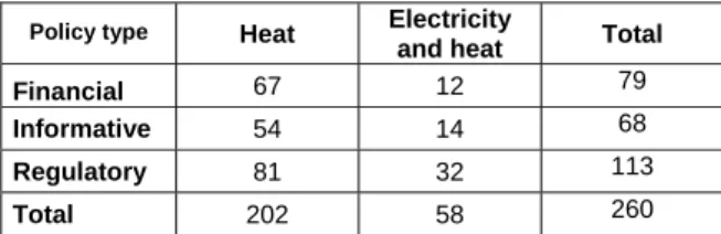
remaining 260 policies, 202 are focused on heat and 58 are focused on both heat and electricity (See Table 18
2). An example of the latter is a policy named “Energy advice for households”, which obviously applies to 19
both heating and other household uses of energy. 20
Table 2 : Numbers of policies from the MURE Policy Database analysed for the purpose of the present worka
21
Policy type Heat Electricity
and heat Total
Financial 67 12 79 Informative 54 14 68 Regulatory 81 32 113 Total 202 58 260 a Categorisation carried out as described in the text. 22
As mentioned earlier, the database of policies and the variable EP are divided into different categories of 23
efficiency policy, to evaluate their respective impacts. The categories chosen are: regulatory, economic, 24
and information policy instruments [41]. According to [42], this classification is based on the degree of 25
authoritative force. Regulations imply commanding particular behaviours; economic instruments aim at 26
altering the benefits and/or costs in order to encourage energy efficiency investments; and, finally, 27
information aims at shifting priorities by building awareness. Several assumptions were needed to apply 28
this categorisation to the policies in the MURE Policy Database. Although policies that are labelled 29
‘Legislative/Informative’ are regulatory, in that they mandate the display of information, these policies 30
have been categorised as informative, since market transformation via information is their main goal. 31
Most of the policies in this category refer to the EU EPBD and the Energy Labelling of Products 32
directives [6, 9]. While the EU EPBD directive contains regulatory components, such as the mandatory 33
11
inspection of boilers, the main focus of both directives is the energy labelling of buildings and appliances, 1
respectively. Policies in the database categorised as ‘Co-operative’ or ‘Unknown’ were each examined in 2
turn to define their placements. Although the Co-operative policy shown in the example for Austria (Table 3
2 ) is ostensibly information-driven, its main contribution with respect to the residential sector is in 4
relation to minimum standards for standby, which makes it a regulatory policy for the classification 5
applied in this work. For some countries, notably, the Netherlands, many of the policies listed are labelled 6
as ‘Co-operative’. This is because in the Netherlands, there is strong representation of housing 7
organisations, which make voluntary agreements with the authorities to reduce energy demand. Each of 8
these polices have been categorised on an ad hoc basis to determine if they are more regulatory or 9
informative in nature. Policies labelled Financial, i.e., grants for renewables, were included. Many of these 10
refer to grants or subsidies for the installation of heat pumps and solar photovoltaic (PV) or collector 11
panels, all of which would reduce the final energy demand, as listed in the energy statistics. Table 2 shows 12
the numbers of policies for each category based on the categorisation carried out for the present work. 13
Most of these policies were implemented in the period 1990–2010, while others were already in force in 14 1990. 15 Table 3 :
Residential sector energy efficiency policies for Austria from the MURE Policy Database [13] analysed in 16 the present work.a
17 Designationb Focusb
Weightb Policy Titlec Policy Typec SQIc Durationc EUc Codec
Financial Heat 20 Residential building subsidy Financial High 1989– No AU13
Heat 20 Grants for renewable energy (heat pumps, biomass etc.) Financial High 1992– No AU10 Heat 1 National recovery plan / renovation voucher Financial Unknown 2009– No AU26
Regulatory
Heat 20 Heating system design standards Legislative/Normative High 1989– No AU6* Heat 20 Minimum thermal standards for buildings Legislative/Normative High 1991– No AU5 Heat 10 Heating cost settlement for common thermal facilities Legislative/Normative Medium 1992– No AU8 Elec 1 EU-related: Energy Labelling (Energy Star) Co-operative Measures Unknown Unknown Yes AU22*
Informative
Heat 20 EU-related: EPBD – Building Energy Certificates Legislative/Informative High 2008– Yes AU21 Heat 20 Klima:Aktiv Building - new standards for buildings Information/Education High 2005– No AU18 Heat 10 ”Wohnmodern“ support for large apartment renovation Information/Education Medium 2006– No AU19*
Heat and
Electricity 1 Energy advice for households Information/Education Unknown 1990– No AU27
Elec 1 topprodukte.at, Platform for energy-efficient appliances Information/Education Low 2005– No AU17* Elec 1 Smart Metering and Informative Billing Information/Education Unknown 2008– No AU28 Elec 10 EU-related: Energy Labelling of Household Appliances Legislative/Informative Medium 1994– Yes AU1
a Since the completion of the work described in this paper, the MURE Policy Database has been reorganised. For the example of Austria given in 18 this table, the reorganisation has resulted in the removal of the policies marked with an asterisk and the relabeling of all household‐focused 19 policies with the prefix HOU, e.g., HOU‐AU13 for the first policy listed in the table. See: http://www.measures‐odyssee‐mure.eu/ 20 b These designations (categories) are assigned as part of the present work. 21 c These items are derived from the MURE Policy Database. 22
As an example, for Austria, the database includes nine heat-focused energy efficiency measures, four 23
electricity efficiency-focused measures, and one measure that covers both heat and electricity. These 24
fourteen policies were introduced between 1989 and 2009 and are all still in force (Table 3). Six of the 25
Austrian measures have received a high SQI, three have received a medium score, one a low score, and 26
four have had their SQI graded as “Unknown”. The policies without an SQI ranking are assumed to have a 27
low impact on demand. The fourteen policies are divided into the Financial (Fin), Regulatory (Reg), and 28
Informative (Info) categories in line with the categorisation used in the present work, although those that 1
focus exclusively on electricity are not included in the subsequent analysis. Columns 1 and 2 of Table 3 2
show the categorisation of the policy measures applied by the authors of this paper, while the remaining 3
columns are based on data from the MURE Policy Database [13]. Thus, Policy Type and SQI are MURE 4
categorisations for each measure. As all the measures are still in force, the column Duration gives the 5
starting year of the policy measure. The column that follows Duration indicates whether the measures 6
were the result of an EU directive or not, while the last column lists the MURE Policy Database codes for 7
Households. 8
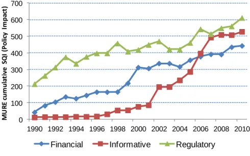
Figure 1 shows the cumulative SQI ranking of the 260 polices analysed in this work. The difference 9
between the numbers shown in Table 2 and those shown in Figure 1 is that rather than show the number of 10
policies in force for the EU-14, the latter takes into account the different rankings assigned to each policy 11
in the MURE Policy Database (high-, medium-, and low-impact policies) and also the years in which each 12
policy was in force. Thus the y-axis of Figure 1 represents the cumulative value of the SQI of the policies 13
in force in each of the three categories for the 14 countries analysed in this work (cf a high-impact policy 14
in force is assigned a value of 20, a medium-impact policy gets a 10, and a low- or unknown-impact 15
policy gets a values of 1). It is clear that informative polices have the lowest expected impact until Year 16
2006 when they catch up with the regulatory policies. A pattern of decreasing impact, e.g., from 1998 to 17
1999 for regulatory policies, reflects the fact that some policies in this category became obsolete in 1998. 18 19 Figure 1 :
Estimated level of impact of each policy category on space heating in the residential sector for the 14 20 EU countries analysed in this work.
21
As it may take several years for the impacts of policies introduced to be realised in terms of energy 22
demand reductions, the EP variable is tested with delays of up to 7 years. This approach of effectively 23
lagging the EP variable also removes the possibility of endogeneity between EP and I for the lagged cases. 24
Bigano et al. [32] and Saussay et al. [31] also incorporated delayed impacts of policies (See Table 1). 25 0 100 200 300 400 500 600 700 1990 1992 1994 1996 1998 2000 2002 2004 2006 2008 2010 MU R E cu m u la ti ve SQ I (P ol ic y Im p ac t)
13
Taking the example of Austria (Table 3), the two pieces of legislation introduced in 1989 would not kick-1
in in the Delay7 scenario until Year 1996, while the six pieces of legislation introduced after Year 2005 2
would not be included in the regression. Note also that in the case of Austria, the flagship EU legislation 3
on energy efficiency in buildings, the EPBD, was only incorporated into policy legislation in Year 2008, 4
which means that its effect, as defined in the empirical examination carried out in this work, is limited. 5
2.3
Data sources for other determinants
6
The data for Eq. (1) for the core determinants of space heating energy demand were obtained from the 7
following sources: income [national private consumption in Euro]; population; average floor area per 8
dwelling; number of permanently occupied dwellings; HDD; energy demand for six energy carriers [coal, 9
oil, gas, district heating, biomass, electricity] for space heating [43]; consumer price indices [private final 10
consumption expenditure deflator] [44]; Harmonized Indices of Consumer Prices (HICP) [45]. Income 11
was divided by population to derive the per capita values. The heating demand data were divided by the 12
total floor area (average floor area per dwelling times the number of permanently occupied dwellings) to 13
derive the heating demand per square metre (unit consumption). IEA [46] provides a time series of prices 14
for the residential sector for coal, oil, gas, and electricity normalised to Year 2005 prices ( €2005/toe), while
15
Werner [47] supplies the time series of prices for district heating. These latter prices were normalised to 16
Year 2005 prices using price indices from the OECD [44] and Eurostat [45]. 17
Combining the time series of prices for these five energy carriers with the corresponding time series of 18
their usage for space heating, from the Odyssee database [43], allowed a Weighted Average Price (WAP) 19
of energy for space heating to be constructed. As a ton of oil equivalent (toe) of oil does not produce the 20
same amount of heat as a toe of natural gas or coal (given their different conversion efficiencies when 21
used in household boilers), the IEA prices for oil, natural gas, and coal were divided by a factor of 0.78, 22
0.85, and 0.64 [48], respectively, to obtain the prices of heat from these respective energy carriers prior to 23
their inclusion in the WAP2. Prices for biomass for the respective countries are not available in national 24
statistics due to the nature of the trade in this commodity. Thus, the options were to include biomass in the 25
energy demand time series (Iit) but not in the weighted average energy price time series or to omit biomass
26
from the energy demand time series; best-fit modelling indicated that the latter option was best. This price 27
time-series thus provides a more accurate estimation of the actual price paid by households for residential 28
sector energy demand than those used in [30-32] (See Table 1). 29
For Finland (1990–1994) and Portugal (1990–1999), no data were available from [43] on the demand for 30
residential sector electricity and space heating respectively. In these two cases, time series for residential 31
sector electricity and total energy demand obtained from [46] and [43] respectively were used to 32
extrapolate the missing data. Prices for district heating were not available for most countries for 2009 and 33
2010. To obtain a complete time series, the district heating prices for each country for Year 2008 were 34 2 These three conversion efficiencies were kept constant for the period of the study. This is due to the assumption that improvements in boiler efficiency over the period were marginal in terms of their impact on overall space heating demand [49].
increased by a factor that corresponded to the change in price of the main heating fuel of the specific 1
country for the period 2008–2010. The justification for this approach is that although district heating can 2
be cheaper than alternative heating fuels, its price is usually maintained just below that of its main 3
competitor. 4
5
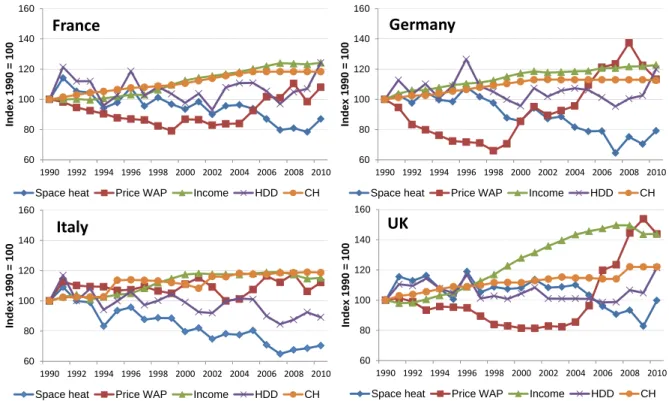
Figure 2 :
Index of space heating demand and determinants of its dynamics (including HDD and penetration of
6
central heating) for four large EU countries.
7
Figure 2 shows the index of unit consumption for space heating demand and for four determinants of 8
energy demand from Eq. (1) for France, Germany, Italy, and the UK, i.e., four of the largest countries of 9
the EU (by demand and population). The dynamics of the variables over the period (Figure 2) shows that 10
unit consumption has been falling since 1990 and that it tracks HDD, with spikes for colder years. Year 11
2010 would appear to have been a very cold year in France, Germany, and the UK. Income per capita and 12
the penetration of central heating have been rising steadily, with the exception of the UK where there was 13
an increase of >50% in income per capita between 1993 and 2008 followed by a fall after the recession. In 14
France, Germany, and the UK, energy prices fell in the 1990’s and rose in the 2000’s, although prices in 15
Italy remained fairly stable for the entire period. In the four countries shown in Figure 2, the penetration of 16
central heating increased by approximately 20% between 1990 and 2010. By Year 2010, the penetration of 17
central heating in the residential sector was >90% in all of the countries examined in the present study, 18
with the exceptions of Greece, Portugal, and Spain [43]. 19 60 80 100 120 140 160 1990 1992 1994 1996 1998 2000 2002 2004 2006 2008 2010 Index 1990 = 100 France
Space heat Price WAP Income HDD CH
60 80 100 120 140 160 1990 1992 1994 1996 1998 2000 2002 2004 2006 2008 2010 Index 1990 = 100 Italy
Space heat Price WAP Income HDD CH
60 80 100 120 140 160 1990 1992 1994 1996 1998 2000 2002 2004 2006 2008 2010 Index 1990 = 100 UK
Space heat Price WAP Income HDD CH
60 80 100 120 140 160 1990 1992 1994 1996 1998 2000 2002 2004 2006 2008 2010 Index 1990 = 100 Germany
15
3
RESULTS AND DISCUSSION
1
This section presents the results of the linear regression of Eq. (1) and discusses the findings in relation to 2
similar studies in the literature. The impacts on demand of the individual variables of Eq. (1) are also 3
described. 4
3.1
Space heating demand per square metre in the period 1990– 2010
5
Table 4 presents the coefficients and test statistics, calculated for the model of space heating demand per 6
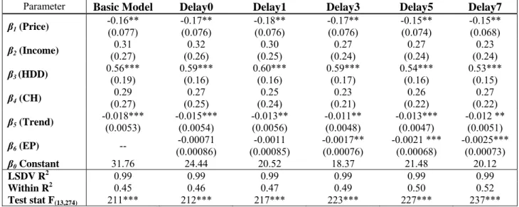
square metre using Eq. (1), for the 14 EU countries examined in the present work. 7 Table 4 :
Elasticity coefficients calculated in models of space heating demand per square metre. The basic model 8 is fitted without any variable for EP. The other models include an EP variable without delay (0) and with delays of 9 1, 3, 5, and 7 years respectivelya.
10
Parameter Basic Model Delay0 Delay1 Delay3 Delay5 Delay7
β1 (Price) -0.16** (0.077) -0.17** (0.076) -0.18** (0.076) -0.17** (0.076) -0.15** (0.074) -0.15** (0.068) β2 (Income) (0.27) 0.31 (0.26) 0.32 (0.25) 0.30 (0.24) 0.27 (0.24) 0.27 (0.24) 0.23 β3 (HDD) 0.56*** (0.19) 0.59*** (0.16) 0.60*** (0.16) 0.59*** (0.17) 0.54*** (0.16) 0.53*** (0.15) β4 (CH) (0.27) 0.29 (0.25) 0.27 (0.24) 0.25 (0.21) 0.23 (0.22) 0.26 (0.22) 0.27 β5 (Trend) -0.018*** (0.0053) -0.015*** (0.0054) -0.013** (0.0056) -0.011** (0.0048) -0.013*** (0.0047) -0.012 ** (0.0051) β6 (EP) -- (0.00086) -0.00071 (0.00085) -0.0011 -0.0017** (0.00076) -0.0021 *** (0.00068) -0.0025*** (0.00073) β0 Constant 31.76 24.44 20.52 18.37 21.48 20.12 LSDV R2 0.99 0.99 0.99 0.99 0.99 0.99 Within R2 0.45 0.46 0.47 0.49 0.50 0.52 Test stat F(13,274) 211*** 212*** 217*** 223*** 227*** 237*** a Values shown in parentheses denote HAC standard errors. ***Significant at 1% level. **Significant at 5% level. *Significant at 10% level. 11
The difference between the six models presented in Table 4 relates to how the time series representing 12
policies focused on energy efficiency (EP)3 are included in the models. In the basic model, EP are not
13
included at all. In the Delay0 model, they are included for the year in which they were published. For the 14
remaining four models, they are included with delays of 1, 3, 5, and 7 years, respectively, after 15
publication. This means that, for example, policies introduced in Year 2000 do not have an effect until 16
Year 2007 in the Delay7 model. The reason for presenting the different models is to compare the effects of 17
the introduction of the EP variable with different time delays. If the values shown in Table 4 for EP are 18
instead calculated as percentages then they represent the percentage reductions in demand for the 19
introduction of one new low-impact policy (e.g., -0.0017 expressed as a percentage is -0.17%.). 20
3
The variable coefficients presented in Table 4 have the expected polarities, in the sense that, for example, 1
when price goes up demand is expected to fall. The price (β1), HDD (β3) and Trend (β5) coefficients are
2
found to be significant at the 5% level for all models. The income (β2) and CH (β4) coefficients are
3
insignificant in all models. Saussay et al. [31] also found the coefficient of income to be insignificant. 4
However, removing Ireland and Portugal from the panel used in the present work resulted in the income 5
elasticity (β2) value increasing to >0.6 and becoming significant at the 5% level4. During the period 1990–
6
2010, these two countries enjoyed large increases in per capita income that were not coupled to any 7
similarly large increases in the use of space heating. It seems that in the absence of economic booms, as 8
experienced in Ireland and Portugal in recent years, the income elasticity for the EU-14 would be higher 9
and significant. Given the lack of statistical significance of the CH variable the F-form of the Wald test 10
was used to examine the effect on the model of omitting it. It was found that the model was not improved 11
by omitting the CH variable5.The F-test for the combined significance of variables was found to be
12
significant at the 1% level for all the models. 13
The absolute values of variable coefficients are also in line with those previously published [16, 31, 33, 14
50, 51], with low price elasticities and slightly higher income elasticities, and with a time trend that 15
represents an annual reduction in demand of >1% per annum. In a static fixed effects panel of electricity 16
demand in the residential sector of 48 US states for the period 1997–2008, Alberini and Filippini [16] 17
deduced price and income elasticities of -0.22 and 0.28, respectively. The values are similar to the results 18
obtained in the present study given the differences in explanatory and dependent variables used. Using a 19
dataset that contains 255 observations in the period 1978–1999, Liu [52] found short-term and long-term 20
price elasticities for total energy demand of -0.025 and -0.140, respectively, for OECD Europe, and short-21
term and term income elasticities for energy of 0.052 and 0.291, respectively. These results for long-22
term elasticities are similar to those found in the present work. Azevedo et al. [34] calculated price 23
elasticities for electricity for the EU of -0.2, which is similar to the value obtained in the present work. 24
EEW [50] reported that autonomous technical progress brings about a 1% per annum reduction in demand 25
across the EU, which corresponds with the coefficients calculated for the time trend in Table 4 and 26
Table 5. Overall, in the present study, the price and income, as well as other calculated elasticities seem to 27
conform to what has been reported in the literature. 28
Although the coefficient of the EP variable is not statistically significant in the Delay0 and Delay1 29
models, it is in the subsequent models. It is clear that as time passes the absolute value and statistical 30
significance of the coefficient of the EP variable increase, while those of the Price, Income, and Trend 31
variables decrease. This suggests that initially the impact of EP on demand is negligible compared to 32 4 Each country was removed in turn from the panel to investigate if there were any significant impacts onβ1 to β6. The above mentioned finding in relation to income elasticity (β2) was the only major deviation from the results presented in Table 4 found. 5
The removal of CH from the model did not change the income elasticity (β2) despite the obvious relationship
between CH and income, i.e. as income rises more households install central heating. The inclusion of CH in the model can be justified because the installation of CH has a non‐linear impact on heat demand, i.e., the installation of CH is said to double the heat demand of an average dwelling.
17
these three other variables but that after a number of years its relative impact increases. During its year of 1
introduction, a low-impact policy reduces demand by 0.071%. This makes sense given that low-impact 2
policies are ranked as those that reduce demand by <0.1% (see Section 2.2). After 5 years, the policy 3
impact has tripled to -0.21% and become statistically significant. 4
Given the disparities in the sizes of the 14 countries included in the panel, e.g., Germany and Ireland, a 5
weighted least-squares regression using the same model variables was used to investigate the size effect. 6
For this, the data for each country were weighted by the square root of its population. This weighting was 7
applied to all the variables, with the exceptions of the time trend and the policy variables. The results 8
obtained were very similar to those shown for the non-weighted models in Tables 3 and 4, suggesting that 9
in this case size does not matter. 10
VIF tests carried out for multicolinearity did not show a VIF value >6 for any variable, indicating that 11
multicolinearity is not a problem for the data and model used. Driscoll-Kraay standard errors [53] were 12
calculated to correct for the possible presence of inter-country spatial correlation in the data set. The 13
calculated Kraay standard errors were smaller than the HAC standard errors. Although Driscoll-14
Kraay standard errors can be biased downwards in small panels, the one used in the present work is in the 15
range suggested by the authors (T>20 and N not important), which suggests that for this dataset, spatial 16
correlation is not a problem. 17
Five different instruments for the EP variable were tested separately to ascertain if the variable was 18
endogenous. The instruments were time series for each country from 1990 to 2010 regarding: 1) the years 19
in which a green political party was in power [54]; 2) the total CO2 emissions [55]; 3) CO2 emissions from
20
the residential sector [55]; 4) gasoline taxes [55]; and 5) average CO2 emissions standards for vehicles6
21
[56]. These five instruments were chosen as possible explanatory variables for the EP variable that were 22
not correlated with energy demand in the residential sector. The idea behind the first three instruments 23
listed was that governments might increase the implementation of efficiency policies as a result of a green 24
party being in government or in reaction to increased CO2emissions. The idea behind the last two
25
instruments was that a regime change in another sector, e.g., transport, might indicate general energy 26
policy development in an unrelated sector, e.g., housing. To determine if EP was endogenous, it was 27
regressed in a model that included one of the five instruments and the other explanatory variables from 28
Eq. (1). The residuals from this auxiliary regression were then added to Eq. (1) as a new explanatory 29
variable that represents the endogenous part of EP. Eq. (1) was then re-run to establish if the endogenous 30
part of EP had statistical significance (Hausman test). This was not found to be the case for any of the five 31
instruments tested, suggesting that EP is not endogenous. 32 33 6 Data for CO2 emissions standards for vehicles for the years 1990 to 1994 and 1996 to 1999 were not available and so were interpolated and estimated based on the data that was available for 1995 and 2000 to 2010.
Table 5 :
Elasticity coefficients calculated in models of space heating demand per square metre. Compared to
1
Table 4, the Efficiency Policies variable (EP) has been divided into three separate types of policy measuresa,b. The
2
basic model is fitted without any variable for EP. The other models include an EP variables without delay (0) and
3
with delays of 1, 3, 5, and 7 years respectively.
4
Parameter Basic Model Delay0 Delay1 Delay3 Delay5 Delay7
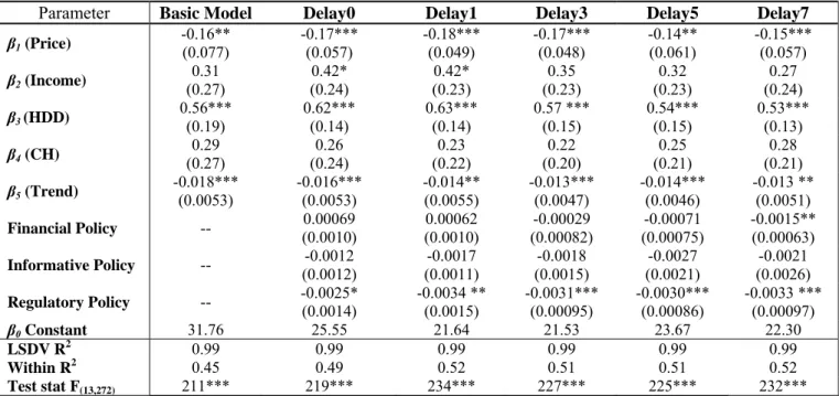
β1 (Price) -0.16** (0.077) -0.17*** (0.057) -0.18*** (0.049) -0.17*** (0.048) -0.14** (0.061) -0.15*** (0.057) β2 (Income) (0.27) 0.31 (0.24) 0.42* (0.23) 0.42* (0.23) 0.35 (0.23) 0.32 (0.24) 0.27 β3 (HDD) 0.56*** (0.19) 0.62*** (0.14) 0.63*** (0.14) 0.57 *** (0.15) 0.54*** (0.15) 0.53*** (0.13) β4 (CH) 0.29 (0.27) 0.26 (0.24) 0.23 (0.22) 0.22 (0.20) 0.25 (0.21) 0.28 (0.21) β5 (Trend) -0.018*** (0.0053) -0.016*** (0.0053) -0.014** (0.0055) -0.013*** (0.0047) -0.014*** (0.0046) -0.013 ** (0.0051) Financial Policy -- (0.0010) 0.00069 (0.0010) 0.00062 (0.00082) -0.00029 (0.00075) -0.00071 -0.0015** (0.00063) Informative Policy -- (0.0012) -0.0012 (0.0011) -0.0017 (0.0015) -0.0018 (0.0021) -0.0027 (0.0026) -0.0021 Regulatory Policy -- -0.0025* (0.0014) -0.0034 ** (0.0015) -0.0031*** (0.00095) -0.0030*** (0.00086) -0.0033 *** (0.00097) β0 Constant 31.76 25.55 21.64 21.53 23.67 22.30 LSDV R2 0.99 0.99 0.99 0.99 0.99 0.99 Within R2 0.45 0.49 0.52 0.51 0.51 0.52 Test stat F(13,272) 211*** 219*** 234*** 227*** 225*** 232*** a Since the OLS regressions technique treats each variable independently, the absolute values of some of the coefficients shown in Table 5 are 5 slightly different from those shown in Table 4. 6 b Values shown in parentheses denote HAC standard errors. ***Significant at 1% level. **Significant at 5% level. *Significant at 10% level. 7
In Table 5, the same models as in Table 4 are presented except that the variable EP is divided into the 8
three policy categories of financial, informative, and regulatory. The polarities and absolute values for the 9
price, income, HDD, CH, and trend coefficients in the models shown in Table 5 are similar to those shown 10
in Table 4. However, examining the statistical significance of the coefficients representing the financial, 11
informative, and regulatory policies shows that only the latter is significant in the Delay0 and Delay1 12
models. This suggests that the coefficient of the EP variable described in the previous paragraph is not 13
significant in the Delay0 and Delay1 models owing to the lack of significance of the impacts of the 14
financial and informative policies. Regulatory policies seem to be the most effective type of energy 15
efficiency policies when the expected impacts, as provided by the MURE Policy Database, are evaluated. 16
The regression coefficients in Table 5 can be interpreted to mean that the introduction of one unit of 17
regulatory policy (i.e., one ‘low-impact’ policy (See Nomenclature and Section 2.2)) has reduced the 18
energy demand by an average of 0.25% in the year of introduction. As this is greater than the <0.1% 19
impact expected for low-impact policies, it can be concluded that regulatory policies have on average 20
performed better than expected. The results also point to different profiles over time for the three policy 21
types: 22
19
Regulatory policies have a strong impact already in the year of introduction, and this impact is 1
consistent over the years that follow. This is what would be expected from policies of this type, 2
e.g., building codes with minimum efficiency requirements. 3
Financial policies show a low impact in the year of introduction, and require a number of years 4
before they reduce demand by >0.1% and reach statistical significance. This might be expected 5
from, for example, subsidies for new technologies whereby more and more house owners adopt 6
the new technology, resulting in a cumulative increase in impact. 7
Information policies show the opposite effect, with an increasing coefficient but falling statistical 8
significance after being in force for 1 year. This may be explained by people getting used to 9
information and returning to previous habits and routines after an initial change of behaviour. 10
The literature on the respective impacts of financial, informative, and regulatory efficiency policies in the 11
residential sector corroborates these findings. Table 5 shows that the correlation between the estimated 12
impact of informative policies from the MURE Policy Database and the savings that actually occurred is 13
low and statistically insignificant. This is similar to previous studies [30, 57], which found that only a 14
small proportion of total annual savings from efficiency at the EU level originated from the effects of 15
information campaigns. In the context of promoting household energy conservation, Steg [58] has 16
reported that information campaigns result in only modest behavioural changes, and von Borgstede et al. 17
[59] has shown that informational policies only give the desired outcomes when households are willing to 18
change wasteful behaviour patterns related to energy use. Yohanis [60] in a survey carried out in Northern 19
Ireland found that although 88% of surveyed homes had purchased a major appliance in the previous 2 20
years, only 16% of the respondents had any idea about the energy ratings of their new appliances. In 21
contrast to these findings, Ek and Söderholm[61] tested the hypothesis that information about available 22
saving measures that is presented in a more concrete and specific way is more likely to affect (stated) 23
behaviour than is more general information. The data they collected from a questionnaire sent to 1200 24
households in Sweden supported this notion. Lindén et al. [62] reported that following repeated 25
information campaigns, households in Sweden filled washing and dishwashing machines before using 26
them and households in detached houses were more likely to adopt a lower indoor temperature than 27
households in apartments. The findings of various groups [61–64] suggest that there is room for 28
improving the design of information polices, although it should be borne in mind that the willingness to 29
switch to pro-environmental behaviours depends on the levels of the perceived thresholds that have to be 30
overcome [59]. 31
The results of interviews with experts and NEEAP screenings [50] revealed enormous disparity across 32
Member States in terms of the levels of ambition of their energy efficiency policies and that in the less-33
progressive countries many experts consider the first EPBD [6] to be a milestone that catalyses a new 34
legal framework for energy use in buildings. Of the portfolio of policy measures in place across the EU, 35
the IEA [64] reported that up to now the EPBD (categorised as an information policy in this work) has 36
been the policy instrument with the greatest potential impact on energy efficiency in existing residential 37
buildings in the short-term ( 5–10-year period) or even in the medium-term up to Year 2020. As the EPBD 38
![Table 1 : Comparisons of the methodologies used in the present study and the previous studies [30‐32].](https://thumb-eu.123doks.com/thumbv2/123doknet/13904159.448314/8.892.32.864.197.1072/table-comparisons-methodologies-used-present-study-previous-studies.webp)