Summary of seakeeping experiments carried out on CCGA Atlantic Swell Model IOT651

(1)

Publisher’s version / Version de l'éditeur:

Vous avez des questions? Nous pouvons vous aider. Pour communiquer directement avec un auteur, consultez la

première page de la revue dans laquelle son article a été publié afin de trouver ses coordonnées. Si vous n’arrivez

Questions? Contact the NRC Publications Archive team at

PublicationsArchive-ArchivesPublications@nrc-cnrc.gc.ca. If you wish to email the authors directly, please see the first page of the publication for their contact information.

https://publications-cnrc.canada.ca/fra/droits

L’accès à ce site Web et l’utilisation de son contenu sont assujettis aux conditions présentées dans le site

LISEZ CES CONDITIONS ATTENTIVEMENT AVANT D’UTILISER CE SITE WEB.

Student Report (National Research Council of Canada. Institute for Ocean Technology); no. SR-2005-08, 2005

READ THESE TERMS AND CONDITIONS CAREFULLY BEFORE USING THIS WEBSITE. https://nrc-publications.canada.ca/eng/copyright

NRC Publications Archive Record / Notice des Archives des publications du CNRC :

https://nrc-publications.canada.ca/eng/view/object/?id=1a9af91c-9041-4c07-a3ec-21ef443f18a7 https://publications-cnrc.canada.ca/fra/voir/objet/?id=1a9af91c-9041-4c07-a3ec-21ef443f18a7

NRC Publications Archive

Archives des publications du CNRC

For the publisher’s version, please access the DOI link below./ Pour consulter la version de l’éditeur, utilisez le lien DOI ci-dessous.

https://doi.org/10.4224/8894842

Access and use of this website and the material on it are subject to the Terms and Conditions set forth at

Summary of seakeeping experiments carried out on CCGA Atlantic Swell Model IOT651

(2)

DOCUMENTATION PAGE REPORT NUMBER

SR-2005-08

NRC REPORT NUMBER DATE

April 2005

REPORT SECURITY CLASSIFICATION

Unclassified

DISTRIBUTION

Unlimited

TITLE

SUMMARY OF SEAKEEPING EXPERIMENTS CARRIED OUT ON CCGA ATLANTIC SWELL MODEL IOT651

AUTHOR(S)

J. Foster

CORPORATE AUTHOR(S)/PERFORMING AGENCY(S)

Institute for Ocean Technology, National Research Council, St. John’s, NL

PUBLICATION

N/A

SPONSORING AGENCY(S)

IOT, CIHR, SAR/NIF

IOT PROJECT NUMBER

42_2017_26

NRC FILE NUMBER KEY WORDS

Seakeeping, Motion Induced Interrupts, Fishing Vessel

PAGES iii, 37, App. A-B FIGS. TABLES 6 SUMMARY

The ‘Atlantic Swell’ is a 35’ inshore fishing vessel. The vessel was built in St. Jones Within, Newfoundland. As part of the National Research Council’s Safer Fishing Vessels project, full-scale seakeeping trials as well as physical model tests were performed on this vessel. The data obtained over the course of these experiments was used to determine various vessel motions in a variety of vessel headings and speeds. The results from each set of trials were compared to determine the correlation between the two tests.

Overall, there was an acceptable level of correlation between both sources. The major dissimilarity between the tests was in the magnitudes of the vessel’s roll angles. All other degrees of freedom examined showed some useful correlation.

ADDRESS National Research Council

Institute for Ocean Technology Arctic Avenue, P. O. Box 12093 St. John's, NL A1B 3T5

(3)

National Research Council Conseil national de recherches

Canada Canada

Institute for Ocean Institut des technologies

Technology océaniques

SUMMARY OF SEAKEEPING EXPERIMENTS CARRIED OUT ON

CCGA ATLANTIC SWELL MODEL IOT651

SR-2005-08

J. Foster

(4)

Summary

The ‘Atlantic Swell’ is a 35’ inshore fishing vessel. The vessel was built in St. Jones Within, Newfoundland. As part of the National Research Council’s Safer Fishing Vessels project, full-scale seakeeping trials as well as physical model tests were performed on this vessel. The data obtained over the course of these experiments was used to determine various vessel motions in a variety of vessel headings and speeds. The results from each set of trials were compared to determine the correlation between the two tests.

Overall, there was an acceptable level of correlation between both sources. The major dissimilarity between the tests was in the magnitudes of the vessel’s roll angles. All other degrees of freedom examined showed some useful correlation.

Major sources of error were determined as a result of this study. These fall under three major categories:

1. Wave Measuring/Matching Issues 2. Model Weight

3. Test Basin Limitations

The most significant of these sources is the wave matching process. Attempting to reproduce something as complicated as a seastate is a very difficult task, even with the best of wave buoys and wave-making equipment. Also, the size of the model did not allow for much flexibility to add ballast to achieve the desired static and dynamic stability attributes.

(5)

This report describes a set of irregular wave seakeeping experiments carried out on a 1:4.697 scale model of the 35 ft. (10.67 m) long inshore fishing vessel the CCGA Atlantic Swell, designated IOT651. The experiments were carried out in the Institute for Ocean Technology (IOT) Offshore Engineering Basin (OEB) in January – February 2005. The data from these tests was used to correlate with the full-scale data acquired during sea trials carried out off St. John’s, NL in October 2003. The summary report of these trials is described in Reference 1. The objective of the experiments was to acquire quality model scale seakeeping data to correlate with the full-scale data.

This document summarizes the model and facility preparation, data acquisition, and data analysis procedures required to provide the results of the ship / physical model correlation exercise. Furthermore, it makes recommendations to improve the overall correlation of similar experiments in the future.

2.0 PROJECT BACKGROUND

This project is a small component of the SafetyNet initiative. SafetyNet is the first federally funded research program investigating occupational health and safety in the historically high risk Atlantic Canada marine, coastal, and offshore industries. The Fishing Vessel Safety Project is conducting research on the occupational health and safety of various fishing vessels. Fishing is the most dangerous occupation in Newfoundland and Labrador. Over the past ten years, the rates of reported injuries and fatalities nearly doubled.

The main focus of this portion of the Fishing Vessel Safety project is to measure Motion Induced Interruptions (MIIs). A MII is an event that causes either an injury or work stoppage because of severe sea conditions. Sea trials and model testing of several fishing

(7)

vessels are being done in order to determine the occurrence and effects of MIIs. This data can be used to determine designs that reduce sudden vessel motions induced by wave action and develop criteria to reduce crew accidents when these motions occur.

The overall results of the project will be represented by a series of recommendations that will provide accessible and applicable information needed to make informed decisions. Additional information on SafetyNet may be found by visiting their web site (Reference 2).

3.0 DESCRIPTION OF PHYSICAL MODEL IOT651

A 1:4.697 scale model, designated IOT651, of the CCGA Atlantic Swell was fabricated at IOT from wood and glass materials. The full-scale Atlantic Swell was not equipped with either a lines plan or a table of offsets. Therefore, Marine Services International Ltd. was contracted to manually measure the full-scale hull offsets. The model was constructed using IOT’s standard model construction procedure described in Reference 3. The model was measured at several key locations to verify dimensional accuracy. This was determined to be within the specified allowable IOT tolerances of ± 0.05% on length and beam and ± 1 mm on section shape.

Model IOT651 included six reference blocks fitted to the gunnels and bow, which were placed at a known elevation relative to the baseline. The model was fully appended with a set of rolling chocks, a single 0.5-inch (1.27 cm) diameter propeller shaft, a flat plate rudder, and a centerline skeg. A four bladed, right-handed turning fixed pitch propeller (#P104R)was used to propel the model. No turbulence stimulators were fitted to the hull or appendages. RENSHAPE reinforcement was bonded to the hull port and starboard forward, well above the waterline, to accommodate two ¾ inch diameter, 8-inch long (1.905 cm * 20.32 cm) aluminum pins. These pins were designed to interact with the model launch system used to accelerate the model to the desired forward speed, in an effort to maximize the available run length in the OEB. An eyebolt was fitted just above

(8)

the waterline on the transverse centerline at the stern to accommodate a tag line used to arrest the model at the end of each run.

The model hull was painted yellow and marked with standard station and waterline markings as described in the model construction standard (Reference 3). It was not anticipated that this model would be tested in a high sea state. This fact was taken into consideration in the model’s watertight integrity strategy. A large lexan hatch was placed over the main deck and rudder servo. It was secured with four quick-release hold clamps to protect the internal electronics in the event that water was to reach this height. A simple superstructure simulating the wheelhouse, open at the top, was included.

The model was propelled by an Aerotech model 1410 motor which was directly connected to the propeller through a watertight stern tube. The maximum continuous rating of the motor is 18 revolutions per second (rps), however this speed could be increased to approximately 22 rps for brief periods. Other outfit components included motor controller, radio control and telemetry electronics, instrumentation, and several batteries of different size and type.

Since this model was relatively small in size, it did not require any additional weight to be added in order to ballast the model. Therefore, the weight and positioning of the batteries was used to keep the model at its draft markings as well as achieve the desired roll/pitch radii of gyration.

The batteries used to power the motor and onboard electronics were smaller than the type commonly used in model testing. When ballasting the model, it was determined that the larger batteries brought the model below its draft markings regardless of where they were positioned. Therefore, a more lightweight type of battery was used. This battery was able to perform for about 4 hours before being changed. Experimentation determined that this battery type did not have quite enough power to reach the 8-knot (full-scale) design speed of the vessel. However, a decision was made to continue with testing using

(9)

the smaller batteries, and arrangements would be made to adjust data to conform with the desired 8-knot design speed.

An inclining experiment was carried out on the fully outfit model in the IOT Tow Tank trim dock. The nominal roll period was checked at this time as well. The disposition of the weight in the model was altered to achieve a compromise between attaining the desired metacentric height and roll period.

The ‘Atlantic Swell’ was not fitted with an autopilot and thus all steering during the sea trials was manual. These same conditions were to be repeated in model scale, thus eliminating the need of fitting an autopilot to the model. An operator located at one end of the tank manually controlled the rudder angle and shaft speed of the model via a radio link.

Model IOT651 was tested in one displacement condition during the model-scale seakeeping trials. This corresponded to the condition recorded during the October 2003 seakeeping trial as described in Reference 1. The closest stability booklet condition to this displacement condition was the 50% consumables condition, however, the actual level of consumables was closer to 40%.

4.0 DESCRIPTION OF THE INSTRUMENTATION

4.1 Model Motions Measurement Instrumentation

Model motions were measured using two independent systems. These are the Systron Donner MotionPak and the QUALISYS system. These two systems used very different principles in order to measure the same parameters. The use of two different systems will allow us to have more confidence in the results obtained.

(10)

1) Systron Donner MotionPak I: Model motions with six degrees of freedom were measured using this unit fitted at the model’s nominal center of gravity. The sensor unit consists of three orthogonal linear accelerometers measuring heave, sway, and surge acceleration (g’s) and three orthogonal angular rate sensors measuring roll, pitch, and yaw rates (degrees/second). One g is approximately equal to 9.808 m/s2.

The three angular rate sensors were calibrated using manufacturer’s data sheets while the three accelerometers were physically calibrated by placing the sensor package on a set of precision wedges machined to defined angles and computing the acceleration relative to the acceleration due to gravity. The sway and surge accelerometers output zero g’s, while the heave accelerometer outputs –1.0 g when the model is level and stationary. This represents the acceleration due to gravity. The intermediate accelerations were computed as follows:

Acceleration = 1.0 * sin (angle of inclination)

2) QUALISYS System: Six infrared emitters were fitted on lightweight Plexiglas masts of varying lengths. These permitted the model to be tracked using an array of 6 cameras located at the east end of the OEB. The system was used to measure the following six motions: orthogonal linear displacements (X, Y, Z) translated to the model CG in a tank ordinate system, heading angle relative to a tank co-ordinate system, and pitch and roll angle in a body co-co-ordinate system. Planar (X, Y) position from the QUALISYS system was used to determine model speed over ground. Calibration of the QUALISYS system is carried out when the system is surveyed using survey points located around the tank.

Although, the components measured by both systems were slightly different, the values of each degree of freedom were integrated appropriately in order to compare both systems.

(11)

Bow Accelerometers

Bow Accelerometers were mounted solely as verification of MotionPak analysis algorithm. The vertical and lateral accelerometers were calibrated the same way as the MotionPak accelerometers and were fitted 150 mm to port, 520 mm forward, and 117.5 mm above the MotionPak.

4.2 Other Instrumentation

Rudder Angle

Rudder Angle is measured by fitting a rotational potentiometer on the pivot point of the rudders. This parameter was calibrated relative to a protractor fitted adjacent to the linkage.

Shaft Rotation

The shaft rotation was measured using a tachometer. The tachometer provides an analog signal linearly proportional to shaft speed and was calibrated using a laser tachometer aimed at a piece of reflective tape on the shaft.

Wave Elevation

Wave elevation was measured using four freestanding capacitance wave probes. Three of which were situated on the south side of the tank while a fourth was located on the north side. The waves were matched using a separate wave probe fitted at a position defined as test center - a central point in the OEB. The locations of the wave measurement probes in the OEB co-ordinate system were:

(12)

South West probe: X = 14.4 m west of test center, Y = 8 m south of test center South Center probe: X = 0 m (test center), Y = 8 m south of test center

South East probe: X = 14.4 m east of test center, Y = 8 m south of test center North Center probe: X = 0 m (test center), Y = 8 m north of test center

Calibration wave probe: X = 0 m, Y = 0 m (test center)

All wave probes were calibrated using the OEB wave probe calibration facility. A sketch of the OEB layout for these experiments is provided in Appendix A.

Data Acquisition

All analog data was low pass filtered at 10 Hz, amplified as required, and digitized at 50 Hz. All data acquired from model sources was conditioned on the model prior to transfer to the shore based data acquisition computer. The wave elevation and QUALISYS data were conditioned/digitized using a NEFF signal conditioner, transferred to the data acquisition system via cable, and stored in parallel with the telemetry data. Synchronization between the NEFF data and telemetry data is nominally within 0.2 s.

An RMS error channel was acquired to monitor QUALISYS signal integrity. Also, the amplitudes of a south and west wave board were acquired to verify wave board activity.

5.0 DESCRIPTION OF THE EXPERIMENTAL SET-UP

The OEB has a working area of 26 m by 65.8 m with a water depth that can be varied from 0.1 m to 2.8 m. Waves are generated using 168 individual, computer controlled wet back wavemaker segments. These are hydraulically activated and fitted along the west and south sides of the tank perimeter. Each segment can be operated in one of three modes of articulation: flapper mode (± 15º), piston mode (± 400 mm), or a combination of both. The wavemakers are capable of generating both regular and irregular waves up to a 0.5m significant height. Passive wave absorbers are fitted around the other two sides

(13)

of the tank. The facility also has extensive video coverage and is serviced over its entire working area by a 5 metric tonne lift capacity crane.

The OEB was specially configured for these experiments. The following conditions were set to achieve desired results for the seakeeping tests:

Water Depth: The water depth was set at 2.8m. Thus, the model was assumed to be operating in deep water (h/T > 4) so there were no shallow water hydrodynamic effects.

Blanking Walls: Blanking walls that can be used to cover the beaches on the north side were removed for all seakeeping experiments.

Segmented Wave Board Configuration: All wave boards were set in piston mode with the bottom of the wavemakers adjusted to 1.3 m above the floor of the OEB.

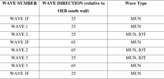
Wave Generation: Several multi-directional irregular waves, corresponding to the waves as measured at sea during the full-scale trials, were matched with dominant wave directions of 25 and 65 degrees relative to the south wall of the OEB. Two wave directions were used to provide some flexibility regarding the model launch direction. The full-scale wave segments were 18 minutes in length.

Two different types of waves were used for the ‘Atlantic Swell’ tests. These corresponded to the two different sets of spreading function characteristics used to generate them. These wave types were denoted the ‘MUN’ wave and the ‘IOT’ wave. The ‘MUN’ wave was used for all run configurations while the ‘IOT’ wave was only used for a few configurations for comparison.

(14)

A listing of the waves used is provided as follows:

WAVE NUMBER WAVE DIRECTION (relative to OEB south wall)

Wave Type

WAVE 1F 25 MUN

WAVE 1 25 MUN

WAVE 2 25 MUN, IOT

WAVE 2F 65 MUN

WAVE 2 65 MUN, IOT

WAVE 3 25 MUN, IOT

WAVE 3 65 MUN

WAVE 3F 25 MUN

Table 1: Wave Types Used in Model Test

In the above table, ‘F’ represents wave spreading angle characteristics ‘flipped’ about their dominant axis. The ability to flip these waves provided additional flexibility with respect to model direction since there was a desire to have specified wave characteristics acting on either the port or starboard side of the model. Full-scale waves from the directional wave buoy emulated in the OEB were acquired as follows:

WAVE #1: acquired Oct. 4, 2003 @ 08:00 Newfoundland time WAVE #2: acquired Oct. 4, 2003 @ 09:30 Newfoundland time WAVE #3: acquired Oct. 4, 2003 @ 10:00 Newfoundland time

Note: WAVE #3 significant wave height with reduced wave heights by 20%. Measured Hm0 = 1.38 m. Reduced Hm0 = 1.245 m.

(15)

Video Cameras:

Four digital video (DV) cameras were used to record the experiments:

1) View #1: camera mounted on a bracket and manually directed from a temporary platform fitted on scaffolding in the tank. The camera position was 1.5 m north of the south waveboards and 11.1 m east of test center.

2) View #2: camera fixed to a temporary platform fitted on scaffolding in the tank. The camera was fitted with a wide-angle lens in order to view the model throughout the run. The camera position was 1.5 m north of the south waveboards and 8.84 m west of test center.

3) View #3: camera mounted in a metal frame on the west wall of the OEB. This camera was situated roughly on the OEB longitudinal centerline and 4.68 m off the floor. The camera was directed remotely (pan, tilt, zoom) by an operator located in the OEB control room.

4) View #4: fixed camera mounted on OEB north walkway directed to view along the model path. This camera was controlled from OEB Control Room.

Note that the View #1 camera was interchanged with the View #2 camera when the model was being launched from the west end of the OEB as opposed to the east end as described above.

Model Launch System

A gravity-based model acceleration system was used to accelerate the model from a standing start in order to maximize the available run length. The model was held in place in a floating cradle that consisted of a ‘U’ shaped aluminum frame accommodating a foam insert conforming to the breadth of the model. Two weights were suspended off

(16)

vertical posts located at the end of the launch system. These were attached to the cradle by a rope and pulley system. This system was used to translate the vertical force imparted by the dropping weights into horizontal thrust on the Aluminum pins located on the port and starboard sides of the model. A lightweight safety line attached from an anchor point on shore to an eyebolt at the model stern was used to arrest the model at the end of the run.

To activate the launch system, two 20 kg weights were manually winched up to a desired height above the tank bottom. For trials in following seas, the size of the weights was decreased, since it required less force to accelerate the model to full speed. Once the weights were suspended at the correct height, the model safety line was attached to a release mechanism. When the mechanism was activated, the weights dropped to the bottom of the tank, and the cradle was accelerated forward. The amount of acceleration required depended on the model heading with respect to the dominant incident waves. The required position and size of the weights was determined experimentally.

6.0 DESCRIPTION OF THE SEAKEEPING TEST PROGRAM

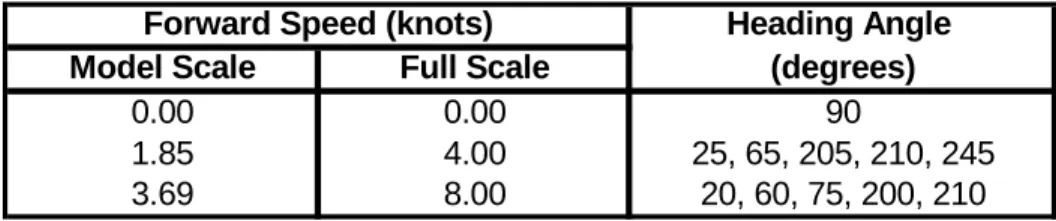
The test program consisted of two different forward speeds (4 knots and 8 knots full scale), each with five headings with respect to the dominant incident wave direction. A 180 degree heading angle is defined has a head sea, while 0 degrees is a following sea. Also, a beam sea drift run was performed. The test plan is summarized in the table below.

Heading Angle Model Scale Full Scale (degrees)

0.00 0.00 90

1.85 4.00 25, 65, 205, 210, 245

3.69 8.00 20, 60, 75, 200, 210

Forward Speed (knots)

(17)

The heading angles were derived after careful examination of the directional wave data and ship heading angle data acquired during the ‘Atlantic Swell’ full-scale seakeeping sea trials. The use of numerical simulations was also used to determine the required headings.

In order to complete trials at all of the headings listed above, the model acceleration system was moved to various locations around the tank. As mentioned, the wavemakers in the OEB have the capability of producing a dominant wave direction that is either 25 or 65 degrees from the south wall. Also, it is possible to move the acceleration system to angles of up to 10 degrees and still achieve the longest possible runs. The model can also be launched from either end of the tank, which gives the ability to complete trials in head, following, beam, bow, or quartering seas.

Whenever the launch system was moved, the model control computer, cabling, and associated equipment were also moved. The ideal control position is behind the launching system so that the model operator can view the entire run from the stern of the model.

6.1 Required Personnel

The following personnel were required to carry out this experiment:

• Operator of video camera view #1 or #2 (whichever provided the better view for the given run direction).

• Model driver operating the model remotely via portable wireless control device. • Individual monitoring the model restraining line and resetting the accelerator after

each run.

• Individual in the OEB control room operating the data acquisition system (DAS) and wave generation computer. This individual was also responsible for manually adjusting video camera view #3 during the actual run.

(18)

• Individual carrying out the online data analysis - reviewing the data after each run using a dedicated workstation in the OEB control room. This procedure is described in the next section of this report.

Often, due to a shortage of available staff, the individual carrying out the online data analysis also operated the manually directed video camera.

6.2 Typical Run Sequence

A typical run sequence is provided as follows:

1) With model in the start position and model launch system weights elevated to their required height, the wave generation signal is loaded and wavemaker span set to 0% stroke.

2) Data acquisition is triggered which commences execution of the wave drive signal. Since the wavemaker stroke is set to 0%, no physical waves are generated at this point. Calm water data is acquired until the required delay interval has passed. Before the model is launched, a suitable period of time is allotted to allow the wave to build and traverse the tank. The process is necessary to ensure the entire spectrum is covered in an efficient manner using a series of wave segments.

3) When the required delay interval has passed, the wavemaker span is increased to 100% and physical wave generation begins.

4) Approximately one minute of waves pass the model with the model constrained in the launcher.

5) Model shaft speed is set at the desired value. The required shaft speed must be reached before the tag line is released and the model is launched.

6) Video recording is commenced on the digital video cameras. 7) The accelerator weights are released and the model launched.

8) The model is propelled down the tank. The rudder angle is controlled by the model operator. The model position is tracked using the QUALISYS system.

(19)

The video camera operator manually tracks the model and zooms in/out as required in order to optimize the image.

9) Within a few meters of the end of the tank, the restraining line arrests the model, and the shaft speed is cut. Video recording is terminated, and wave generation and data acquisition are stopped.

10) The model is towed manually back to the starting position using the tag line. The propulsion system/rudder control is used to maneuver the model back into the launcher. A wait time of 12 minutes between runs is required to permit the tank to settle to calm.

11) The process is then repeated as many times as required to complete the 1200 seconds (full-scale) sequence. This usually takes approximately 12 runs for 4-knot sequences and 24 runs for the 8-4-knot sequences.

The zero speed drift runs were executed by setting the model at a 90 degree angle to the incident waves near the west end of the tank and acquiring data until the either model drifted too close to an obstructions or the tank perimeter, or acquisition of 18 minutes full-scale data was complete. No tag line was connected to the model during drift speed runs.

In addition to the runs in waves, a number of roll decay experiments were carried out in calm water at zero forward speed as well as 4 and 8 knots. The model was manually stimulated in roll by depressing the main deck at the maximum beam. Pitch decay runs were also carried out at zero forward speed in calm water by manually depressing the bow to stimulate the model in pitch.

(20)

7.0 DATA ANALYSIS

7.1 Online Data Analysis

All of the data for the seakeeping experiment was acquired in GDAC format (*.DAC files) described in References 6, 7. At the end of each run, the data acquired was analyzed in the period of time allotted for tank settling. This analysis ensured that all sensors and data acquisition equipment was functioning and providing reasonable results. No detailed data analysis was performed at this point. The online data analysis command procedure was executed for each test as follows:

• All measured channels were converted from GDAC to GEDAP format (described in Reference 8) in full-scale units. GEDAP is the software used by IOT to analyze data from model tests.

• QUALISYS data was de-spiked to remove some signal dropouts.

• MotionPak motion analysis software was run, generating six degree of freedom motions at the model center of gravity (CG) in an earth fixed co-ordinate system. Since the MotionPak unit was fitted at the model center of gravity, it was not necessary to transfer the computed motions to a new location. The accelerations, velocities, and displacements of all six vessel degrees of freedom were output, thus resulting in the following 18 channels: three orthogonal angular accelerations/rates/angles (roll, pitch and yaw) and three orthogonal linear accelerations / velocities /displacements (surge, sway and heave).

• A routine was executed to transform QUALISYS linear displacements (X, Y, Z) to the model CG.

• A routine was executed to compute two speed channels (in full scale m/s and knots) from QUALISYS planar position data.

• All data was plotted in the time domain and time segments for statistical analysis were interactively selected.

(21)

• The following time series were plotted for review:

o Plot #1: six QUALISYS acquired model motion channels (3 orthogonal linear displacements, roll, pitch and heading angle)

o Plot #2: six MotionPak acquired model motion channels (3 orthogonal linear accelerations, 3 orthogonal angular rates)

o Plot #3: QUALISYS signal integrity channel, south wave board monitoring channel and the four wave probe channels

o Plot #4: model speed over ground (m/s), rudder angle, shaft speed, bow vertical and lateral acceleration channels

o Plot #5: computed MotionPak motion channels – (3 orthogonal angles, 3 orthogonal linear displacements)

• Basic statistics (minimum, maximum, mean, standard deviation) were computed for all measured and computed channels for each selected time segment.

• The five time series plots and a table of basic statistics was output to a local laser printer in the OEB Control Room and statistics were stored in the project directory.

The data collected above was used in performing the online analysis. The following is a list of parameters examined throughout the course of this analysis. These give a good indication of the quality of the data acquired.

• The value of the shaft rps, model forward speed, heading angle were verified as conforming to the input values. Since the model was not equipped with an autopilot, an acceptable heading angle for a given run was the judgment call of the person performing the online analysis.

• The standard deviation of the motion channels measured by QUALISYS and MotionPak were compared.

• The signal integrity channels were reviewed for evidence of signal loss. If significant signal loss was detected during critical segments of the run, the run was repeated.

(22)

• The pitch and roll angle data from QUALISYS and the integrated roll and pitch rate data from MotionPak were plotted over the same time scale and compared.

7.2 Offline Data Analysis

The data from the model test in GEDAP format, was scaled from model-scale to full-scale using the scaling factor. Most of the data channels could be used directly after they have been scaled, however, modifications were required to achieve better data on some channels. For example, the rudder angle and shaft speed channels were low pass filtered using a high frequency cut-off value of 3 Hz to remove signal noise. Also, the QUALISYS data was de-spiked to remove some dropouts. The spikes seen on the QUALISYS data are a result of the tracking cameras losing sight of the markers located on the model.

An extended time segment was selected on the six acquired MotionPak channels. This time segment consisted of the run time plus 100 seconds added to both the beginning and the end of the run. This is because the first 5% and last 5% of the data is discarded due to the merging process used.

A routine was executed to transform QUALISYS linear displacements (X, Y, Z) to the model center of gravity. QUALISYS motions were derived from an origin located at the base of the stern marker for run sequences 1 – 3. Therefore, motions were moved 4.2495 m forward, 0.7866 m down (full-scale), in order to transfer the origin to the center of gravity. QUALISYS motions were derived at the center of gravity for run sequence 4 – 10 and all drift runs, so no correction was required.

In order to smooth out anomalies in the QUALISYS data, a 3 degrees of freedom (DOF) polynomial can be fit to the QUALISYS X and Y displacement channels. A routine was executed to compute the model speed channels (m/s, knots) from QUALISYS planar position (X, Y) data. Then, a 3 DOF polynomial can be fit to the derived model speed

(23)

channel (knots). Also, a routine was executed to transform the MotionPak yaw angle to the wave incident angle.

Now that all of the required corrections have been made, all of the data is in the required form, and analysis can be done. The following 16 channels are enough to cover the full range of data analysis required for the seakeeping experiment:

# Channel Description Units

001 North Center Wave Probe m 002 Shaft RPM rpm 003 Rudder Angle deg. 004 MP_Surge_Displacement m 005 MP_Surge_Acceleration m/s2 006 MP_Sway_Displacement m 007 MP_Sway_Acceleration m/s2 008 MP_Heave_Displacement m 009 MP_Heave_Acceleration m/s2 010 MP_Heading_Angle deg. 011 MP_Yaw_Velocity deg./s 012 MP_Pitch_Angle deg. 013 MP_Pitch_Velocity deg./s 014 MP_Roll_Angle deg. 015 MP_Roll_Velocity deg./s 016 Speed knots

Table 3: Output Channels used for Data Analysis

The following process was used to complete the offline analysis for the seakeeping model experiments of the Atlantic Swell:

• Organize run log such that the end time of one run is the same as the start time of the following run. Repeat this process for all runs in each sequence.

• Write command procedures to be used for data analysis using IOT’s VMS data analysis software.

• Copy run files to the appropriate location within VMS and enter required information. This includes the start and end time of the run, the MotionPak extended time segment, QUALISYS location transfer coordinates, and heading angle transform. This gives an output of 16 different files (one per channel) for each run.

(24)

• Merge all runs together for each sequence with three seconds overlap between runs. This should ensure a relatively smooth transition. The result is one file for each channel that spans the entire 18-minute full-scale wave spectrum.

• Each of the merged channels can be plotted in the time domain and reviewed, taking note of any abnormalities. In some cases, more overlap was needed between runs. Also, some spikes were removed by selecting the beginning and end of the glitch and using linear interpolation to fill the gap. Any major motion anomalies such as large transient motions at the beginning of a run, were identified and avoided during further analysis.

• Once all the spikes and anomalies were removed, the basic statistics (minimum, maximum, mean, standard deviation) were computed for all channels. This information was output in tabular form.

8.0 COMPARISON OF FULL-SCALE AND MODEL TEST DATA

A comparison between the results of the full-scale sea trials data described in Reference 1 and physical model data collected, is presented in this section. An initial correlation of the seakeeping data with full-scale trials results, preliminary physical model results and numerical predictions is provided in Reference 5.

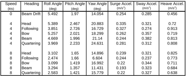
A summary of full-scale sea trials data from Reference 1 is given in Table 4, while summary results for the model tests are presented in Table 5. Comparison plots of vessel motions measured full scale and model scale versus heading angle are provided for forward speeds of 4 knots and 8 knots in Appendix B.

(25)

Speed Heading Roll Angle Pitch Angle Yaw Angle Surge Accel. Sway Accel. Heave Accel.

(kts) (deg) (deg) (deg) (m/s2) (m/s2) (m/s2)

0 Beam Drift 5.492 1.97 14.054 0.254 0.285 0.456 4 Head 5.389 2.467 20.883 0.335 0.321 0.72 4 Following 3.851 2.726 16.729 0.327 0.274 0.913 4 Bow 5.257 2.021 18.299 0.262 0.357 0.719 4 Beam 4.669 1.996 21.14 0.244 0.382 0.813 4 Quartering 3.969 2.233 24.631 0.281 0.312 0.808 8 Head 3.102 1.65 14.896 0.239 0.321 0.825 8 Following 2.474 1.66 6.604 0.244 0.237 0.773 8 Bow 3.099 1.419 16.992 0.22 0.344 0.711 8 Beam 3.294 1.357 11.431 0.193 0.323 0.684 8 Quartering 2.583 1.421 15.779 0.22 0.327 0.638

Table 4: Summary of Standard Deviations of Motions in Full-Scale Sea Trial

Several Conclusions can be made from Table 4. These are listed as follows:

• Roll and pitch motions are less significant for the 8-knot ship speed compared to the 4-knot speed.

• Roll motions are greatest when the ship is in either head, bow, or beam seas. This corresponds to vessel headings of 90 – 270 degrees.

• Pitch motions are greatest in head and following seas, and are smallest in beam waves.

• Yaw angles are reduced as vessel speed increases.

• Yaw angles are smallest in following seas. It is difficult to determine any other trend with regards to yaw angles and vessel headings. It is expected that larger yaw angles will occur in beam or quartering seas if the majority of wave energy comes from the dominant direction. This is shown in the 4-knot trials, but not in the 8-knot trials. It is likely that wave conditions changed in the time between the two sets of trials.

• Surge Acceleration is lower for the 8-knot case than the 4-knot case.

• Surge Acceleration is largest in head and following seas. This is the expected result since a vessel is more likely to experience fore and aft accelerations when going directly into or with the waves.

(26)

• Sway Acceleration is smallest in following seas. We would expect sway acceleration to be greatest in beam seas. This is seen in only the 4 knot case. • Heave acceleration decreases as speed increases for most vessel headings. No

other noticeable trends are seen on the Heave Acceleration channel with regards to vessel speed or heading. Heave Accelerations are mostly influenced by the wave heights and periods observed at the time of the trial.

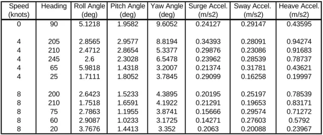
Speed Heading Roll Angle Pitch Angle Yaw Angle Surge Accel. Sway Accel. Heave Accel. (knots) (deg) (deg) (deg) (m/s2) (m/s2) (m/s2)

0 90 5.1218 1.9582 9.6052 0.24127 0.29147 0.43595 4 205 2.8565 2.9577 8.8194 0.34393 0.28091 0.94274 4 210 2.4712 2.8654 5.3377 0.29876 0.23086 0.91683 4 245 2.6 2.3028 6.5478 0.23962 0.28539 0.78737 4 65 5.9818 1.4318 3.2007 0.21374 0.31781 0.43621 4 25 1.7111 1.8052 3.7845 0.29099 0.16258 0.19997 8 200 2.6423 1.5233 4.3895 0.20195 0.25197 0.78539 8 210 1.7518 1.6591 4.1922 0.21291 0.19653 0.83171 8 75 2.7863 1.1955 3.8741 0.15666 0.29574 0.71272 8 60 2.9087 1.0233 3.1725 0.14271 0.27603 0.5792 8 20 3.7676 1.4413 3.352 0.2063 0.20088 0.23967

Table 5: Summary of Standard Deviations of Motions for Model Test Data

Table 5 is in a slightly different format than Table 4. The main difference being the vessel headings listed. When testing at sea, the actual wave direction was difficult to determine. Therefore, it was impossible to acquire data in pure head, following, or beam seas. Therefore, the model scale runs were focused on obtaining results for a range bow and quartering seas. In order to compare the model test data to the full-scale data, we will make some approximations. These are summarized in Table 6.

able 6 – Heading Approximations for Model-Scale Data

Actual Heading (deg.) Heading Approximation

20, 25 Following 60, 65 Quartering 75, 245 Beam 210 Bow 200, 205 Head T

(27)

A comparison between the full-scale and model test results can now be made.

• The model test results show a very large roll value for a speed of 4 knots in

• smaller in the model tests compared to the full-scale

• m and

• riations with heading for model • angles decreased with speed increase for all headings. This is in keeping • eas, and were smallest in quartering

•

This indicates a form of human error present on the sea trials. Since the vessel was not equipped with Comparisons are listed as follows:

quartering seas. This does not correspond well to the result seen at sea. This may be due to excitations produced by the non-dominant wave, or any of the factors listed later in this paper.

Overall, roll angles were

trials for the 4-knot condition. This may be because the smaller waves may not have enough energy to produce the excitations required to cause larger roll.

Roll angles decreased with speed increase for most cases except for the bea

quartering waves. A generally accepted result is that roll decreases with vessel speed increase for all headings. Discrepancies may be due to the variation in heading approximation between the two speeds.

There was no noticeable trend for roll angle va tests.

Pitch

with the results obtained from the sea trials. Pitch angles were largest in head and bow s

seas. This result is slightly different that obtained in sea trials. In regular waves, it is obvious that a vessel will pitch most in head or following seas. Although regular waves do not occur in nature, this result was seen in the sea trials. This indicates that the vast majority of wave energy came from the dominant direction when the sea trials were done. There are two reasons why the results may be slightly different in model scale: First, we did not actually test in head or following seas, so the full effect of pitching in these seastates is not felt. Second, the wave matching process is very difficult. Since ocean waves are very random, many parameters need to be estimated in order to match waves.

Yaw angles decreased with speed increase for all headings • Yaw angles are much smaller than those noted on sea trials.

(28)

an autopilot, the vessel was steered manually. It is likely that the vessel captain instinctively steered the vessel in a way to reduce roll and pitch. Therefore, as a result, the vessel heading was quite variable, which lead to larger yaw angles. Yaw angles are smallest in quartering and following seas. Yaw angles are expected to be small in head and following seas. The variability in yaw ang •

les

•

• is greatest in headings near head and following seas. This is in

•

ration was more noticeable for the

4-following seas. This trend was not noticed in the sea trials; however,

Overall t results between the

o sets of trials. In order to interpret the data correctly, we must determine why some

otions decreased as vessel speed increased. This is an expected trend. Generally, a vessel will experience largest motions when sitting still in the seen in these tests is mostly a result of how the vessel was steered. It was not expected that conclusive results for yaw angles would be obtained in these tests because they are greatly influenced by the vessel’s course. With a manually steered vessel, the ability to maintain course depends largely on the abilities of the captain. The use of an autopilot would give a better understanding of vessel behavior in yaw.

Surge acceleration decreases as vessel speed increases. Surge acceleration

keeping with the sea trials and the expected data. • Speed has little effect on sway acceleration.

Sway acceleration is smallest in following seas. • The effect of vessel heading on heave accele

knot trials.

• Heave acceleration is greatest in near-head seas and decreases as the vessel approaches

it is not uncommon for vessels to experience this behavior.

, the data collected shows some consistent and inconsisten tw

parameters showed similar results and why some did not. Once this is known, efforts can be made to correct the inconsistencies and improve the model testing process.

8.1 Consistent Results

(29)

water. As the vessel speed increases, it’s susceptibility to large motions decreases.

Yaw angle and surge acceleration decrease as vessel speed increases. Yaw angles

•

• are smallest in following seas. This trend was observed even though ommon for

•

• mallest in following seas.

ted that since sway and show similar results. The fact

8.2 Inc

odel test were smaller than full-scale for the 4-knot condition. This is likely due to a lack of roll excitation experienced in the smaller waves of

•

n determined the exact cause of the large discrepancies seen on the roll consistent results were less likely to be achieved on this channel. It is c

yaw to be smallest in following seas. This means that the wave-matching process is relatively accurate.

Surge Acceleration is largest in head and following seas. Sway Acceleration is s

• Speed has little effect on Sway Acceleration. It is expec yaw are both lateral vessel motions, they should

that this was not seen may be related to the fact that no autopilot was used. For the 4-knot case, yaw was very high. If course was maintained, some of this yaw motion may have been seen in the form of sway. Therefore, the higher yaw may have lead to lower sway for the 4-knot condition.

onsistent Results

• Roll angles in the m the OEB.

Full-scale and model test roll angles varied differently with vessel heading. It has not yet bee

channel. It is believed that one source of error is the roll radius of gyration. Although, it was attempted to match this parameter to the full-scale value, many sources of error were encountered. First, the weight constraints on the model meant that it was impossible to match this parameter exactly to the vessel without compromising other important vessel characteristics. Second, since the ‘Atlantic Swell’ was not built conforming to a lines plan, the exact roll radius of gyration for the full-scale vessel is not known exactly. Therefore it will be difficult to overcome these factors to achieve accurate results.

(30)

•

e to difficulties in wave matching. It requires some human

9.0 DATA CORRELATION DISCUSSION

en data collected full-scale and model-ale, using a scaled geosimilar physical model. In the case when a new ship design has

f the modeling process is to generate data that reflects the results ollected full scale, the experimentalist must be aware of the factors that degrade the full Model test yaw angles are much smaller. Again, this is due to the fact that there was no autopilot.

• Model test heave accelerations lower for following/quartering headings. This result may be du

observation and extrapolation in order to determine the most appropriate dominant and non-dominant wave directions, and how much energy is associated with each.

Ideally, there would be a perfect correlation betwe sc

not yet been implemented, the designer would rely on the model testing process in order to determine the seakeeping characteristics of the ship. The situation outlined in this report is different. Here, the design has already been implemented, and full-scale data has been collected. The purpose of this study is to determine how much merit can be put towards the model testing process when it comes to small coastal fishing vessels. Therefore, if we are to have any faith in the model testing process, there must be some useful correlation between the data collected at sea, and the data collected using the model. This being said, we must keep in mind that neither test is perfect. Each test has its strengths and weaknesses. A goal of the correlation process is to determine which test is more accurate for each individual parameter and why.

9.1 Full Scale Data

Although the goal o c

scale data. This must be taken into consideration when evaluating the integrity of the overall correlation. The factors that are believed to have degraded the full-scale data set collected on the ‘Atlantic Swell’ are discussed in this section.

(31)

• No Autopilot

Thi m ssel was not fitted with an autopilot and thus the entire trial was arried out using manual steering. The steering was somewhat erratic in nature with yaw

on Wave Buoy Accuracy at Low Frequency s s all fishing ve

c

angles often exceeding ± 40 degrees and standard deviation in the order of 15 to 25 degrees. The physical model was also manually controlled in order to match the full-scale condition, however, the yaw angles recorded were generally less than ± 10 degrees. It was also noted that the quality of the steering, both full scale and model scale, varied with the skill and experience of the operator. The difference in steering control between the full-scale ship and the physical model will likely have a significant negative impact on the correlation.

• Limitations

Win g to 30 s with the longest

period waves being generated by very strong winds that blow for long periods from a

ted from the roll/pitch otion of the buoy using standardized techniques such as those described in Reference 9.

d enerated ocean waves have a period ranging from 2 s

constant direction. The majority of the wave energy comes from the direction from which the wind is blowing. Lower energy waves are created at angles away from the primary wind direction. The magnitude of this energy decreases as these angles increase. Weak winds produce only short wave length, high frequency waves, that tend to die out quickly. On the other hand, large storms can produce a low frequency swell that can propagate large distances from the storm center. In the area where the waves are generated, directional spreading is relatively large, with a considerable portion of the waves propagating to the sides of the predominant wind direction.

Directional wave data acquired by the MUN wave buoy is calcula m

In low frequency waves, the signal-to-noise ratio in the buoy instrumentation can be so small that wave direction is not measured accurately. If this is the case, the waves matched in the model test will be inaccurate and results will be affected.

(32)

• Variation in Full Scale Sea State with Time

Loc s o the influence of variation in wind peed/direction, current, tide and other influences. On the October 2003 sea trial, the sea

Wave Buoy Mooring Issues

al ea conditions are constantly changing due t s

was fairly confused and the wave direction was also changing over time. This is not uncommon especially since the trial was carried out near an irregular coastline. Trials were completed as quickly as possible in order to reduce the effects of changing sea states.

•

The MUN wave buoy was originally designed for short-term deployment from small oats to supply data in support of near-shore naval operations. Due to the nature of the b

trial, the buoy was moored at specified location. It is likely that the integrity of the wave height data may be compromised due to this effect. An alternative strategy would be to deploy the buoy free floating, although this would involve additional complications and risks.

• Wave Buoy Failure

The Neptune wave buoy failed during the trial before all of the required data was ollected. An attempt was made to linearly extrapolate the data based on the observed

Direction c

trend (Reference 1). Therefore, only a rough estimate of wave conditions is available for some of the 8 knot runs. This lack of acquired wave data is assumed to have a significant negative impact on the correlation.

• Estimation of Dominant Wave

Loc y or more low frequency swells. Swells riginating in other areas and locally generated waves often emanate from different

all generated waves often co-exist with one o

(33)

directions and thus result in several peaks in the wave energy spectrum. The result is a confused sea where the dominant wave direction is difficult to determine. On the ‘Atlantic Swell’ trial, the dominant wave direction was assessed visually at the start of each forward speed run sequence, and once defined, the vessel proceeded on the specified five courses with respect to the waves (see diagram below). During the trial, it became apparent that the dominant wave direction was either changing with time or was not defined correctly.

• Spatial Variation in Wave Field

The mo ve height and direction at a single point however is safe to assume that there is a spatial variation in these parameters throughout the

un 1: Head Sea un 2: Following Sea

Sea

• Variation of Ship’s Speed

ored wave buoy measures the wa it

trials area. The variation in wave characteristics was mitigated by the fact that the water depth was relatively constant throughout the trials area. In addition, a run pattern as recommended by the ITTC (Reference 10) was adopted such that data was collected as close to the moored wave buoy as possible.

R R

Run 3: Bow Sea Run 4: Beam Sea Run 5: Quartering

Du ping trial, an effort was made to maintain a constant peed over ground for a given heading angle with respect to the incident wave. Once the appropriate shaft speed had been selected, it remained constant throughout the run.

ring the October, 2003 seakee s

(34)

Nominal shaft RPM and measured speed over ground (from Reference 1) are listed as follows:

Head Sea: Shaft RPM: 227, Forward Speed: 4.0621 knots Bow Seas: Shaft RPM: 262, Forward Speed: 4.069 knots

eam Seas: Shaft RPM: 325, Forward Speed: 4.235 knots ots nots

eam Seas: Shaft RPM: 506, Forward Speed: 8.404 knots nots nots

ard speed by varying the B

Quartering Seas: Shaft RPM: 335, Forward Speed: 4.281 kn Following Seas: Shaft RPM: 303, Forward Speed: 3.904 k

Head Sea: Shaft RPM: 541, Forward Speed: 7.901 knots Bow Seas: Shaft RPM: 553, Forward Speed: 7.438 knots B

Quartering Seas: Shaft RPM: 583, Forward Speed: 7.341 k Following Seas: Shaft RPM: 574, Forward Speed: 7.800 k

Thus, even though there was an effort to maintain constant forw shaft speed, some variation in forward speed was noted.

• Variation in Static Stability, Draft

As the trial progresses, the vessel is burning fuel oil and using other consumables. This may e with a resulting change in static and dynamic tability characteristics, as well as a small change in draft. Other activities being carried

result in some variation in free surfac s

out by the crew during the trial may also have an undesirable impact on the ship’s condition. On a small vessel such as the ‘Atlantic Swell’, even crew members moving around during the trial would have some impact on the static stability.

(35)

• Estimate of Static Stability (GMT)

n inclining experiment was carried out on the ‘Atlantic Swell’ two days prior to the sea tria vessel (Reference 1). The experiment was

omplicated by the fact that there is very limited information available for this vessel. It A

l to estimate the static stability of the c

was never possible to match the model LCG to that provided in the inclining report.

• Inherent GPS Inaccuracies:

IOT used the Global Positioning System (GPS) with a differential correction from a Canadian Coast Guard source to provide the most accurate data available for determination of the ship’s course and speed over ground (COG, SOG). Although efforts were made to acquire the best data possible, there are still significant errors introduced when using a GPS.

• Location/Alignment of Sensors

One of the challenges when installing sensors on a ship is accurate determination of their loc inate system. Normally, the position of motion nsors (MotionPak, accelerometers, etc.) and the GPS antenna are referenced relative to

• Model Geometry

ation and alignment in a ship co-ord se

the nominal center of gravity and/or aligned with the ship’s longitudinal axis. There were few alignment references on the ‘Atlantic Swell’ and thus only a rough alignment of the sensors was possible.

9.2 Physical Model Data

odels are milled from foam using computer generated tool paths and glassed as describ . The hull offsets for the ‘Atlantic Swell’ were obtained from M

(36)

manual measurements as there were no drawings of the vessel available. The displacement of the faired hull derived from these offsets could not be matched:

• IOT Stock Propeller

The IOT stock propeller selected for use on the Model #IOT651 was close to the desired iameter, however it rotated in the opposite sense to the propeller installed on the ship.

ake d

This resulted in an induced hydrodynamic yaw moment opposite to the one experienced on the ‘Atlantic Swell’.

• Propeller Shaft R

The shaft rake on the model was determined from the CAD drawing to be 4 degrees owever due to an error in interpreting the information provided from the contractor, the

ttributes h

actual shaft rake was supposed to be 3.62 degrees.

• Setting Model Stability and Displacement A

One of is including all the required utfit items in a small volume without exceeding the defined displacement limit or

T: 28.72 cm Achieved GMT: 29.25 cm

arget Roll Period: 1.487 s Achieved Roll Period: 1.476 s the greatest challenges in outfitting a physical model

o

deviating from the correct draft and trim. Also, we must position weights to ensure that the desired static and dynamic stability attributes are met. For the ‘Atlantic Swell’ experiments, no ballast weight was required. Therefore, there was little flexibility available to adjust the model’s static and dynamic stability. Adjusting the layout of the batteries was the only means available to attain the desired weight distribution. In the end, a compromise between achieving the model scale target GMT and roll period was

required:

Target GM T

(37)

NOTE: roll period as determined for zero forward speed in OEB.

• Wave Matching Issues

The a lated to emulating a real multi-directional wave spectrum the OEB that impact the overall quality of the generated wave:

of the tank and there is a spatial variation in the wave parameters over the tank area.

ll experiments although there was some variation in

-

ency was approximately 0.31 Hz and it was

-

in any testing basin.

• Propul

re re a number of issues re in

- The wave is matched at a single point in the center

- Some errors are introduced when a number of segments are combined to make up a single run.

- Only three waves acquired during the morning of October 4th were matched and used for a

wave properties noted full-scale over the time frame of the data collection. A constant spreading angle is selected whereas the real spreading angle was also changing with time.

- The challenge in emulating the high frequency wave components in the OEB. The full-scale roll frequ

not possible to include significant energy at this frequency due to limitations of the OEB wavemakers.

Although efforts were made to reduce the effects of wave reflection off of tank walls, this effect will be present

sion Motor Power

There was insufficient power available on the model to propel the model at 8 knots full ale. The maximum achievable speed was 7.3 to 7.6 knots full-scale depending on sc

(38)

• Forward Speed Control

For essel’s forward speed will vary over the course of an regular wave as the ship encounters periods of relative calm followed by a series of

• Uncertainty in Instrumentation a fixed shaft speed, the v ir

higher waves. Since a number of runs are required to cover the entire spectrum, there is a variation in forward speed between runs. Some experimentation was required to determine a suitable shaft speed; however, it may take extensive testing to determine the most appropriate speed.

A d i rement uncertainties inherent in a physical model otions instrumentation package is described in detail in Reference 11. Both systematic

eta led investigation into the measu m

(fixed) and random (precision) uncertainties associated with measured motions (roll angle, pitch angle, and heave acceleration) were calculated. The analysis indicated that total uncertainties are in the 1-2% range. Compared to other sources of error, the uncertainties created in the instrumentation and data acquisition are relatively small.

• Merging Data

Wh d using the dedicated merging process, it was obvious that some arameters varied significantly throughout the run. The most notable of these was the

en data was merge p

model’s speed over ground. Each run showed either an accelerating or decelerating trend throughout the run. This meant that the speed data collected over the course of each sequence not completely consistent. Although the mean of the speed values shows the expected value, the data shows consistent sharp oscillations. It is obvious that because of significant changes in speed throughout the run, the merged speed data is not in keeping with what was observed on the sea trials.

(39)

• MotionPak and QUALISYS Comparison

A comp S roll angle, pitch angle, yaw/heading ngle and vertical (heave) displacement was completed. The results show that there is an

0.0 CONCLUSIONS

of the model testing of the ‘Atlantic Swell’, many observations ere made regarding vessel behavior. Any time that this type of correlation exercise is

rces of error were identified. For the full-scale akeeping trials, the most important issue was the integrity of the wave data. The

cult process to emulate a real multi-directional wave field in a latively small test basin. It is obvious that attempting to model a parameter, which is influenced by so many factors, such as a wave spectrum, will introduce large degrees of

arison between MotionPak and QUALISY a

excellent comparison between the angular data with less than 0.5% difference in standard deviation. A difference in yaw/heading angle standard deviation of approximately 3% would likely be improved if the QUALISYS markers could be placed farther apart on the model. It was determined that the integrity of the QUALISYS data is influenced by model position and/or orientation in the OEB tank co-ordinate system. The vertical (heave) displacement comparison is poor (> 30% difference in standard deviation). One factor contributing to this poor relationship includes the fact that the MotionPak heave acceleration signal is double integrated and thus somewhat degraded, however the large difference warrants further investigation.

1

Throughout the course w

completed, something new is learned about the model testing process, even if the data does not correlate as well as expected.

As previously noted, a number of sou se

variation of the wave field with time, the spatial variation of the wave field, as well as issues associated with the wave buoy combine to provide a challenge in quantifying the wave conditions present.

It is known that it is a diffi re

(40)

uncertainty. Dedicated research is required to address these issues, and collaboration with other wave basins facing similar challenges is recommended.

The other major limitation related to carrying out seakeeping experiments in the OEB is the relatively short run lengths and small model scale. Ongoing efforts are underway to

evise test strategies to mitigate the negative aspects of the small basin size.

hough some rogress has been made in reducing the weight of conventional models, additional

seen in vessel motion data throughout the trials. The xception to this is the roll angle. The reasons why such different results were seen on d

With regards to model weight issues, it is now known that more flexibility is required in order to match parameters such as the natural roll period of a vessel. Alt

p

recommendations would include replacing the motor controller with a modern lightweight unit and replacing the rudder servo with a modern digital unit with programmable azimuth rate.

Despite all of the errors present, some good correlation was made between the two sets of trials. Similar trends were

e

the roll angle channels are still unknown. Some further investigation should be done to determine why the roll data does not correlate as well as other channels. The recommendations made in this paper should be used in conjunction with the results of other similar studies in order to reduce errors in the future.

(41)

11.0 REFERENCES

1) Barrett, J, Cumming, D., Hopkins, D.,”Description of Seakeeping Trials Carried tlantic Swell – October 2003”, IOT Trials Report #TR-2003-28, December 2003.

2)

ww.SafetyNet.MUN.ca

Out on CCGA A

“SafetyNet – a Community Research Alliance on Health and Safety in Marine and Coastal Work”, w , February 2005.

ort #TR-2004-01, January 2004.

4) els

ore Structures and Propellers”, V7.0, 42-8595-S/GM-1, August 2, 2002. 11

5)

land Fleet”, 23rd International Conference on Offshore Mechanics and Arctic Engineering (OMAE), June 2004, Vancouver, BC. 13

6)

, January 2, 1996. 16

7)

itute for Marine Dynamics Software Design Specification, Version 3.2, August 14, 1996. 17

3) Cumming, D., Hopkins, D., Barrett, J.,”Description of Seakeeping Trials Carried Out on CCGS Shamook – December 2003”, IOT Trials Rep

Institute for Ocean Technology Standard Test Method: “Construction of Mod of Ships, Offsh

Bass, D., et al,”Assessing Motion Stress Levels on Board Fishing Vessels of the Newfound

Miles, M.D.,”Test Data File for New GDAC Software”, NRC Institute for Marine Dynamics Software Design Specification, Version 3.0

Miles, M.D.,”DACON Configuration File for New GDAC Software”, NRC Inst

(42)

8) Miles, M.D.,”The GEDAP Data Analysis Software Package”, NRC Institute for

9) Steele, K.E., Teng, C.C., Wang, W.C., “Wave Direction Measurements Using Mechanical Engineering, Hydraulics Laboratory Report No. TR-HY-030, August 11, 1990. 18

Pitch-Roll Buoys”, Ocean Engineering, Volume 19, Issue 4, pp. 349-375, 1992. 20

10) Proceedings of the 22nd ITTC, Vol. II, Seoul, Korea & Shanghai, China,

11) Hermanski, G., Derradji-Aouat, A., Hackett, P., ”Uncertainty Analysis – dian

6, September 5 -11, 1999. 21

Preliminary Data Error Estimation for Ship Model Experiments”, 6th Cana Marine Hydro-mechanics and Structures Conference, Vancouver, BC, May 23-2 2001. 23

(43)

(44)

(45)

(46)

(47)