Analytic model for matched-filtered scattered intensity of volume inhomogeneities in an ocean waveguide calibrated to measured seabed reverberation

Analytic Model for Matched-filtered Scattered

Intensity of Volume Inhomogeneities in an Ocean

Waveguide Calibrated to Measured Seabed

Reverberation

MA

by

Anamaria Ignisca

Submitted to the Department of Mechanical Engineering

in partial fulfillment of the requirements for the degree of

Master of Science in Mechanical Engineering

at the

MASSACHUSETTS INSTITUTE OF TECHNOLOGY

SSACHUSETTS INSTITUTE OF TECHNOLOGY

JUL 2

9

2011

LIBRARIES

ARCHVES

June 2011

@

Massachusetts Institute of Technology 2011. All rights reserved.

A uthor ...

...

Department of Mechanical Engineering

May 20, 2011

.1

(

Certified by...

. .~... ...- . .. 7..-.-.... ... .... . . ...

Nicholas C. Makris

Professor of Mechanical Engineering

Thesis Supervisor

Accepted by

... ...- : .. .... Y . . " ...

David E. Hardt

Graduate Officer, Department of Mechanical Engineering

Analytic Model for Matched-filtered Scattered Intensity of

Volume Inhomogeneities in an Ocean Waveguide Calibrated

to Measured Seabed Reverberation

by

Anamaria Ignisca

Submitted to the Department of Mechanical Engineering on May 20, 2011, in partial fulfillment of the

requirements for the degree of

Master of Science in Mechanical Engineering

Abstract

In this thesis, we derive full theoretical expressions for the moments of the matched filtered scattered field due to volume inhomogeneities in an ocean waveguide and pro-vide a computationally efficient time harmonic approximation to the matched filtered model. Following the approach developed by Galinde et al 16], the expressions are de-rived from first principles, by applying Green's theorem and the Born approximation. The scattered field and the total moment expressions are in terms of the fractional changes in the bottom compressibility and density, as well as the waveguide Green function and its gradients. The volume inhomogeneities are assumed to be statisti-cally stationary, and assumed to be correlated in all three directions following a delta correlation function. Sound propagation in the ocean is modeled using the parabolic equation model and actual measurements of bathymetry and sound speed at the ex-perimental locations. Monte Carlo simulations are used to account for the sound speed variability in the ocean waveguide due to internal waves or other sources of acoustic field randomization. The computationally efficient time-harmonic model is shown to provide a good approximation to the full broadband matched filtered model for a standard Pekeris waveguide. The time-harmonic model is then calibrated for ocean bottom reverberation at several frequencies in the 415-1325 Hz band, with data collected during the 2003 and 2006 ONR Geoclutter Experiments on the New Jersey continental shelf and on the northern flank of Georges Bank in the Gulf of Maine, respectively. The statistics for the inverted bottom parameters are summarized for all frequencies and experimental locations considered. The acoustically determined bottom parameters are shown to vary with approximately the wavelength cubed, suggesting that, by different frequencies selecting the scale of the acoustic inhomo-geneities, the acoustic effects dominate over the geophysical effects.

Thesis Supervisor: Nicholas C. Makris Title: Professor of Mechanical Engineering

Acknowledgments

I would like to thank my thesis advisor, Professor Nicholas C. Makris, for the support and guidance he offered on preparing this thesis and throughout my academic career at MIT. I am grateful for the lessons Professor Makris taught me and my fellow students not only in class, but also in the lab, through encouraging us to make progress one step at a time and to learn through discovery.

I would also like to thank Dr. Mark Andrews, Prof. Purnima Ratilal, and Hadi Tavakoli Nia for laying the ground work for the material in this thesis, and for the guidance and direction they offered at the onset of this endeavor.

To Geoff Fox, Leslie Regan and Joan Kravit I thank for their help with all the logistics related to preparing this thesis and completing my degree at MIT.

My colleagues and friends at MIT have also played a crucial role in the devel-opment of this work. Srinivasan Jagannathan, Ankita Deepak Jain, Dong Hoon Yi, Wenjun Zhang, Kalina Gospodinova, Audrey Maertens and Derya Akkaynak Yellin have always been there when I had questions related to acoustics or needed moral support.

Lastly, I would like to thank my parents, brother and husband for their love, support, and understanding.

Contents

1 Introduction 21

2 Analytic Formulation 23

2.1 Matched filtered scattered field ... ... 24

2.2 Full analytical expressions for the total moments of the matched filtered scattered field . . . . 26

2.3 Time harmonic approximation to the matched filtered scattered intensity 32 3 Model implementation for a Pekeris waveguide 35 3.1 Approximations to the matched filtered scattered intensity . . . . 36

3.2 Frequency dependence of simulated reverberation . . . . 44

4 Model calibration to bottom reverberation data 53 4.1 OAWRS bottom reverberation data . . . . 53

4.2 Parameter inversion methodology . . . . 55

4.3 Model/data comparison using beam time data . . . . 57

4.4 Model/data comparison using polar plots . . . . 62

4.5 Statistics and frequency dependence of inverted parameter . . . . 64

5 Conclusion 69

A Matched filtered total moment expressions based on conditional

mo-ments 71

C Examples of calibration results for C.1 New Jersey, 415 Hz . . . . C.2 New Jersey, 925 Hz . . . . C.3 New Jersey, 1325 Hz . . . . C.4 Georges Bank, 415 Hz . . . . C.5 Georges Bank, 950 Hz . . . . C.6 Georges Bank, 1125 Hz . . . . each experiment . . . . . . . . . . . . . . . . . . . . and frequency 85 86 91 96 101 106 111

List of Figures

3-1 Pekeris waveguide with sand bottom, where c,,,, p, and a,, are the sound speed, density and attenuation of the water column, and cb, pb and ab are those of the sea-bottom. The water column sound speed

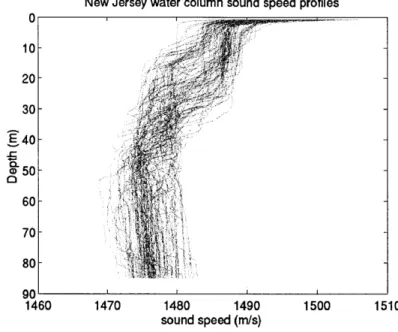
profiles used in simulations are actual sound speed profiles measured on the New Jersey continental shelf [16]. . . . . 36 3-2 The sound speed profiles measured on the New Jersey continental shelf. 37 3-3 Total moments of the full 390-440 Hz matched filtered scattered field

in a Pekeris sand waveguide with varying sound speed profiles, for 10 realizations of the ocean environment. The level of the mean squared term is dependent on the number of realizations and on the range

increment dr, while the level of the variance term is stable. . . . . 38 3-4 Total moments of the full 390-440 Hz matched filtered scattered field

in a Pekeris sand waveguide with varying sound speed profiles, for a single realization of the ocean environment. For the case of a single realization, the total moments are equal to the moments conditional on a set of deterministic Green functions. . . . . 39 3-5 Total 390-440 Hz matched filtered variance and its terms in a Pekeris

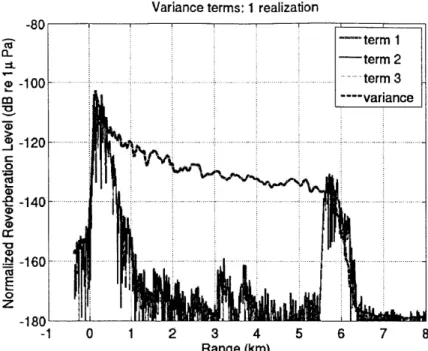
sand waveguide, for 10 realizations of the ocean environment . . . . . 40 3-6 Total 390-440 Hz matched filtered variance and its terms in a Pekeris

sand waveguide, for a single realization of the ocean environment. For a single realization, the last two terms cancel each other and the total variance is equal to the conditional variance . . . . . 41

3-7 Full 390-440 Hz matched filtered depth-integrated monostatic bottom reverberation compared to time harmonic reverberation at center fre-quency 415 Hz, for 10 realizations of the ocean environment. ... 42 3-8 Full 390-440 Hz matched filtered depth-integrated monostatic bottom

reverberation compared to time harmonic reverberation at center

fre-quency 415 Hz, for a single realization of the ocean environment. . . . 42

3-9 Range-averaged full 390-440 Hz matched filter depth-integrated monos-tatic bottom reverberation compared to range-averaged time harmonic reverberation at center frequency 415 Hz, for 10 realizations of the

ocean environment (range averaging over 500 m). . . . . 43 3-10 Range-averaged full 390-440 Hz matched filter depth-integrated

monos-tatic bottom reverberation compared to range-averaged time harmonic reverberation at center frequency 415 Hz, for a single realization of the ocean environment (range averaging over 500 m). . . . . 43 3-11 Range-averaged full 390-440 Hz matched filter bottom reverberation

compared to its three terms: monopole, dipole and crossterm (range averaging over 500 m). . . . . 45 3-12 Range-averaged time harmonic bottom reverberation at center

fre-quency 415 Hz compared to its three terms: monopole, dipole and crossterm (range averaging over 500 m). . . . . 45 3-13 Range averaged time-harmonic simulated monostatic reverberation level

in a sand Pekeris waveguide with isovelocity sound speed profile, at 16km from source/receiver (range averaging over 2000m). . . . . 46 3-14 Range-averaged time-harmonic simulated monostatic reverberation level

in a sand Pekeris waveguide with isovelocity sound speed profile, at 415,

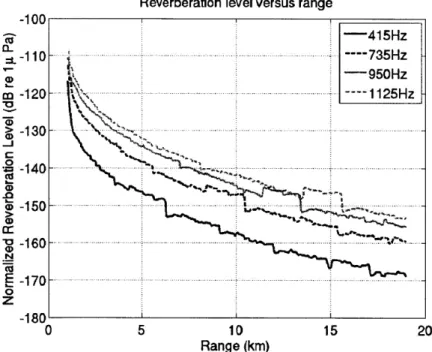
735, 950 and 1125 Hz, respectively (range averaging over 2000 m). . . 47

3-15 Range-averaged time-harmonic simulated monostatic reverberation level in a sand Pekeris waveguide with isovelocity sound speed profile, for all frequencies, at 4, 10 and 16 km in range, respectively (range averaging

3-16 Frequency dependence of time-harmonic simulated monostatic rever-beration level at 16 km in range for a sand Pekeris waveguide with isovelocity sound speed profile (range averaging over 2000 m), for bot-tom parameters V, Var(IT(rt)), Var(Fd(rt)) and Covar(F,,(rt)) con-stant for all frequencies. . . . . 49 3-17 Volume integral from Equation 3.3 plotted versus frequency for several

locations in range . . . . 49 3-18 Frequency dependence of volume integral from Equation 3.3. ... 50 3-19 Value of the integral in Equation 3.3 evaluated at several depths: the

integration is performed over a bottom layer that is 0.1 m thick, as

dz = 0.1 m . . . . 51 3-20 Value of the integral in Equation 3.3 evaluated from the 100 m

wa-ter/air interface down to several depths: the integration is performed over all 0.1 m thick bottom layers located between 100 m and the depths indicated in the legend . . . . 51 4-1 OAWRS image charting returns (dB re 1 pPa) received on the Northern

Flank of Georges Bank at 18:31 EDT, on 3 October 2006. The white diamond indicates the source and the black line is the receiver track. The white curves are bathymetric contours for the region. Clutter is distinguished from seafloor returns by inspecting both the bathymetry of the region and the stationarity of the returns over multiple pings. Ship beams are also identified as radiating outward from the receiver, symmetrically about the endfire of the receiver array. . . . . 54 4-2 Measured normalized pressure level as beam time series for the New

Jersey continental shelf (left) and Georges Bank in the Gulf of Maine (right). The black stars indicate the beams chosen for analysis. The source is broadband for 415 Hz center frequency and 50 Hz bandwidth and the source level is normalized to 0 dB re 1 pPa at 1m. . . . . 57

4-3 (Left) Bathymetric map of the New Jersey continental shelf indicating the source and receiver positions at 10:31 EDT, on 13 May 2003. The grey diamond indicates the source, located at 39.2312N, 72.8818W and operating at 390-440 Hz. The black diamond indicates the receiver, located at 39.2465N, 72.8626W, with heading 346*E. The black and magenta stars indicate the beams chosen for analysis, corresponding to the original and mirror beams, respectively. (Right) Bathymetric map of the northern flank of Georges Bank in the Gulf of Maine indicating source and receiver positions at 11:58 EDT, on 26 September 2006. The grey diamond indicates the source, located at 41.8901N, 68.2134W and operating at 390-440 Hz. The black diamond indicates the receiver, located at 41.8212N, 68.3368W, with heading 137*E. The black and magenta stars indicate the beams chosen for analysis, corresponding to the original and mirror beams, respectively. . . . . 58 4-4 Parameter estimates 0 (log scale) estimated from the data pings shown

in Figure 4-2 for the New Jersey (left) and Georges Bank (right) exper-iments, at 415 Hz. Each 0 corresponds to one beam and was estimated using Equation 4.6, where the summation is performed over all n res-olution cells Vs, along the beam. Typically, each beam extends for 25 to 35 km in range, which leads to values of n from 1667 to 2333, respectively, given the sonar range resolution of 15 m. The mean of the parameter estimates (0) is indicated by the red horizontal line and is obtained using Equation 4.7, with p = 1 and m representing the number of beams in each ping. For this figure, m equals 31 and 36 for the New Jersey and Georges Bank experiments, respectively. . . . . . 60 4-5 Model/data comparison along one beam for pings received at center

fre-quency 415 Hz during the New Jersey (left) and Georges Bank (right) experiments, respectively. The source level is normalized to 0 dB re 1 pPa at 1 m . . . . 61

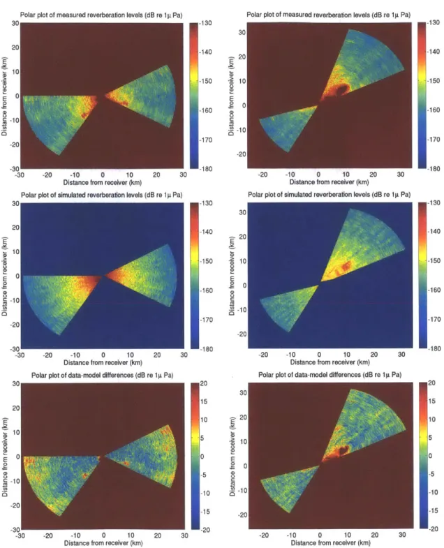
4-6 Model/data comparison along one beam for pings received at center fre-quency 415 Hz during the New Jersey (left) and Georges Bank (right) experiments, respectively (range averaging over 2000 m). The source level is normalized to 0 dB re 1 pPa at 1 m . . . . 62 4-7 Polar plots of measured reverberation level (top), simulated

reverbera-tion level (middle) and their difference (bottom) for New Jersey (left) and Georges Bank (right). The source level is normalized to 0 dB re 1 [tPaatlm... ... 63 4-8 Histogram of the data-model differences as show in Figure 4-7 (bottom)

for New Jersey (left) and Georges Bank (right). For the New Jersey errors (left), the mean is -1.1467 dB and the standard deviation 6.5095 dB. For the Georges Bank errors (right), the mean is -0.3526 dB and the standard deviation 5.8003 dB. . . . . 64 4-9 Histograms of parameter values (log scale), for the New Jersey (left)

and Georges Bank (right) data. . . . . 66 4-10 Mean (dots) and standard deviations (error bars) for the parameter

estimate 0, as given in Table 4.1, for the New Jersey and Georges Bank data . . . . 67 4-11 Mean parameter estimates 0 (circles), as given in Table 4.1, for the

New Jersey and Georges Bank data, along with least squares fitted lines for each experiment. . . . . 67

B-1 Real part (left) and source spectrum

Q(f)

2 for 1 second long LFM (top), CW (middle) and Gaussian (bottom) waveforms. . . . . 80 B-2 Simulated reverberation level using the first term of the matched

fil-tered total variance for 10 Monte Carlo simulations, after normalization by rB, for LFM, CW and Gaussian 1 second long broadband pulses centered at 415 Hz and with 50 Hz bandwidth. . . . . 81

B-3 Total matched filtered variance and its three terms, for 1 second LFM, CW and Gaussian broadband pulses centered at 415 Hz with 50 Hz bandwidth. . . . . 82 B-4 Second term of total variance (Equation 2.18) for 1 Monte Carlo

sim-ulation, for CW pulses of 1 to 7 second duration, centered at 415 Hz and with 50 Hz bandwidth. . . . . 83

C-1 Parameters obtained after fitting the model to the data for each beam, in log scale. The red horizontal line indicates the mean of the param-eter values (log scale). Only beams corresponding to relatively flat or downward sloping bathymetry were included in the analysis. Endfire beams as well as beams contaminated by clutter were also excluded. The second half of the data and model time series were chosen for calibration, as the model fails to predict well the data for small ranges. 86 C-2 list entry . . . . 87 C-3 Comparison of measured and simulated reverberation levels plotted

against: beam time (top), range from the receiver along the original beam (middle), range from receiver along the mirror beam (bottom), for beams 30, 40 and 50, indicated by magenta stars in Figure C-2 (top right). ... ... 88 C-4 For the same beams as in the previous figure C-3: comparison of

mea-sured and simulated reverberation time series after range/time averag-ing (top); comparison of the monopole term before addaverag-ing the

rever-beration intensities for the original and mirror beams (bottom). . . . 89

C-5 Histogram of data-model differences for Figure C-6. . . . . 89 C-6 Beam time (left) and polar (right) plots of measured reverberation

level (top), simulated reverberation level (middle) and their difference (bottom ). . . . . 90

C-7 Parameters obtained after fitting the model to the data for each beam, in log scale. The red horizontal line indicates the mean of the param-eter values (log scale). Only beams corresponding to relatively flat or downward sloping bathymetry were included in the analysis. Endfire beams as well as beams contaminated by clutter were also excluded. The second half of the data and model time series were chosen for calibration, as the model fails to predict well the data for small ranges. 91 C-8 list entry . . . . 92 C-9 Comparison of measured and simulated reverberation levels plotted

against: beam time (top), range from the receiver along the original beam (middle), range from receiver along the mirror beam (bottom), for beams 30, 40 and 50, indicated by magenta stars in Figure C-8 (top right). . . . . 93 C-10 For the same beams as in the previous figure C-9: comparison of

mea-sured and simulated reverberation time series after range/time averag-ing (top); comparison of the monopole term before addaverag-ing the

rever-beration intensities for the original and mirror beams (bottom). . . 94

C-11 Histogram of data-model differences for Figure C-12. ... 94 C-12 Beam time (left) and polar (right) plots of measured reverberation

level (top), simulated reverberation level (middle) and their difference (bottom ). . . . . 95 C-13 Parameters obtained after fitting the model to the data for each beam,

in log scale. The red horizontal line indicates the mean of the param-eter values (log scale). Only beams corresponding to relatively flat or downward sloping bathymetry were included in the analysis. Endfire beams as well as beams contaminated by clutter were also excluded. The second half of the data and model time series were chosen for calibration, as the model fails to predict well the data for small ranges. 96 C-14 list entry . . . . 97

C-15 Comparison of measured and simulated reverberation levels plotted against: beam time (top), range from the receiver along the original beam (middle), range from receiver along the mirror beam (bottom), for beams 30, 40 and 50, indicated by magenta stars in Figure C-14 (top right). . . . . 98 C-16 For the same beams as in the previous figure C-15: comparison of

measured and simulated reverberation time series after range/time av-eraging (top); comparison of the monopole term before adding the reverberation intensities for the original and mirror beams (bottom). . 99 C-17 Histogram of data-model differences for Figure C-18. . . . . 99 C-18 Beam time (left) and polar (right) plots of measured reverberation

level (top), simulated reverberation level (middle) and their difference (bottom ). . . . . 100 C-19 Parameters obtained after fitting the model to the data for each beam,

in log scale. The red horizontal line indicates the mean of the param-eter values (log scale). Only beams corresponding to relatively flat or downward sloping bathymetry were included in the analysis. Endfire beams as well as beams contaminated by clutter were also excluded. The second half of the data and model time series were chosen for calibration, as the model fails to predict well the data for small ranges. 101 C-20 list entry . . . . 102 C-21 Comparison of measured and simulated reverberation levels plotted

against: beam time (top), range from the receiver along the original beam (middle), range from receiver along the mirror beam (bottom), for beams 25, 37 and 42 indicated by magenta stars in Figure C-20

(top right). . . . . 103 C-22 For the same beams as in the previous figure C-21: comparison of

measured and simulated reverberation time series after range/time av-eraging (top); comparison of the monopole term before adding the reverberation intensities for the original and mirror beams (bottom). . 104

C-23 Histogram of data-model differences for Figure C-24. . . . .1

C-24 Beam time (left) and polar (right) plots of measured reverberation level (top), simulated reverberation level (middle) and their difference (bottom ). . . . . 105

C-25 Parameters obtained after fitting the model to the data for each beam, in log scale. The red horizontal line indicates the mean of the param-eter values (log scale). Only beams corresponding to relatively flat or downward sloping bathymetry were included in the analysis. Endfire beams as well as beams contaminated by clutter were also excluded. The second half of the data and model time series were chosen for calibration, as the model fails to predict well the data for small ranges. 106

C-26 list entry . . . . 107

C-27 Comparison of measured and simulated reverberation levels plotted against: beam time (top), range from the receiver along the original beam (middle), range from receiver along the mirror beam (bottom), for beams 35, 45 and 50, indicated by magenta stars in Figure C-26

(top right). . . . . 108

C-28 For the same beams as in the previous figure C-27: comparison of measured and simulated reverberation time series after range/time av-eraging (top); comparison of the monopole term before adding the reverberation intensities for the original and mirror beams (bottom). . 109

C-29 Beam time (left) and polar (right) plots of measured reverberation level (top), simulated reverberation level (middle) and their difference (bottom ). . . . . 110

C-30 Parameters obtained after fitting the model to the data for each beam, in log scale. The red horizontal line indicates the mean of the param-eter values (log scale). Only beams corresponding to relatively flat or downward sloping bathymetry were included in the analysis. Endfire beams as well as beams contaminated by clutter were also excluded. The second half of the data and model time series were chosen for calibration, as the model fails to predict well the data for small ranges. 111 C-31 list entry . . . . 112 C-32 Comparison of measured and simulated reverberation levels plotted

against: beam time (top), range from the receiver along the original beam (middle), range from receiver along the mirror beam (bottom), for beams 35 and 45, indicated by magenta stars in Figure C-31 (top right). . . . . 113 C-33 For the same beams as in the previous figure C-32: comparison of

measured and simulated reverberation time series after range/time av-eraging (top); comparison of the monopole term before adding the reverberation intensities for the original and mirror beams (bottom). . 114 C-34 Beam time (left) and polar (right) plots of measured reverberation

level (top), simulated reverberation level (middle) and their difference (bottom ). . . . . 115

List of Tables

3.1 Statistical geologic properties of the New Jersey Strataform, as esti-mated by Galinde et al [6]. . . . . 37 4.1 Table showing the results of the parameter estimation. The first two

columns represent the corresponding center frequencies and experiment locations, respectively. The number of pings, p, and total ping-beam samples, mp, used in the analysis are given in the third and fourth columns, respectively. The next six columns give the mean (level and log scale), standard deviation (level and log scale), as well as the per-centage of beam samples within one and two standard deviations, re-spectively. One 0 is estimated for each single beam in each single ping using Equation 4.6, where the summation is performed over all n reso-lution cells Vs, along the particular beam. As mentioned in Figure 4-4, we typically sum over 1667 to 2333 resolution footprints along each beam. Then, the mean parameter estimate (6) is obtained by averag-ing the parameter estimates 0 over all mp paverag-ing-beam samples, as given by Equation 4.7. (* the NJ and GB symbols stand for New Jersey and Georges Bank, respectively) . . . . 65

Chapter 1

Introduction

The ability to accurately predict reverberation level in the ocean for different sediment types and frequency ranges is critical for remote sensing and imaging systems. The reverberation in shallow continental shelf environments for moderate sea surface wind conditions, has been shown to be mainly due to scattering from the ocean seabed [22], [19]. Several methods have been developed to model bottom scattering, including interface roughness scattering models, based on the roughness at the water-bottom interface [19], [21], [4], and volume scattering models, for scattering due to seabed volume inhomogeneities [6], [19], [23], [11], [12], [20]. For areas of relatively flat bathymetry and for the shallow grazing angles associated with low frequency long-range reverberation, it has been shown that volume scattering is the dominant factor in total bottom reverberation [17], [20], [10]. Models for scattering from volume inhomogeneities in the ocean seabed have been formulated in the literature, but have generally not included the matched filter, which is applied in remote sensing systems to "provide high-resolution imaging of the seafloor and submerged targets" [3]. The matched filter "allows for scatterers extending over multiple range resolution cells of the imaging system to be automatically localized in range, and does not require to artificially break-up the scatterers to within each range resolution cell, as in the case of time-harmonic or other broadband models" [1].

In this thesis, we derive full theoretical expressions for the moments of the matched filtered scattered field due to volume inhomogeneities and provide a computationally

efficient time harmonic approximation to the matched filtered model. Following the approach developed by Galinde et al

[6],

the expressions are derived from first princi-ples, by applying Green's theorem and the Born approximation. The scattered field and the total moment expressions are in terms of the fractional changes in the bottom compressibility and density, as well as the waveguide Green function and its gradients. The volume inhomogeneities are assumed to be statistically stationary, and assumed to be correlated in all three directions following a delta correlation function. Sound propagation in the ocean is modeled using the parabolic equation model RAM [5], and actual measurements of bathymetry and sound speed at the experimental locations. Monte Carlo simulations are used to account for the sound speed variability in the ocean waveguide due to internal waves or other sources of acoustic field randomiza-tion. The computationally efficient time-harmonic model is shown to provide a good approximation to the full broadband matched filtered model for a standard Pekeris waveguide. The time-harmonic model is then calibrated for ocean bottom reverber-ation at several frequencies in the 415-1325 Hz band, with data collected during the 2003 and 2006 ONR Geoclutter Experiments on the New Jersey continental shelf and on the northern flank of Georges Bank in the Gulf of Maine, respectively [16], [15]. The statistics for the inverted bottom parameters are summarized for all frequencies and experimental locations considered.

This thesis is structured as follows: In Section 2, we present the analytic formu-lations for the moments of the matched filtered scattered field and a time harmonic approximation. In Section 3, we implement the matched filtered and time harmonic formulations to a standard Pekeris waveguide, using bottom parameters estimated by Galinde et al [6] for the New Jersey continental shelf. Here, we show that the time-harmonic model provides a good approximation to the matched filtered model and we investigate the frequency dependence of the time-harmonic model while keeping the bottom parameters constant. In Section 4, we calibrate the computationally effi-cient time-harmonic model to ocean reverberation data and present statistics for the inverted bottom parameters at several frequencies and at two different geographical locations.

Chapter 2

Analytic Formulation

In this section, we derive analytic expressions for the total moments of the matched filtered scattered field from random volume inhomogeneities extending over multiple resolution cells in range. We start by deriving the scattered field in terms of the single frequency

f.

We then apply the matched filter and use Fourier synthesis to obtain the time dependent matched filtered scattered field. Next, we derive full formulations for the total scattered field moments, and indicate that the matched filtered scattered intensity can be approximated by the incoherent term. We also provide a computationally efficient time harmonic approximation to the matched filtered scattered intensity.

We consider an ocean waveguide consisting of a water layer, located between an air halfspace above, and a bottom halfspace below. We let (x, y, z) be the coordinates of a cartesian coordinate system with origin at the air-water interface, and the z-axis pointing down. We place the source at ro=(xo, yo, zo), the receiver at r=(x, y, z), and the center of the inhomogeneity at rt=(xt, yt, Zt).

f

represents the frequency,

w = 27rf the angular frequency, c the sound speed, and k = w/c is the acoustic wave number.

2.1

Matched filtered scattered field

To derive the matched filtered scattered field from random volume inhomogeneities, we follow the approach developed by Morse and Ingard [18] and Galinde et al [6], and start from the inhomogeneous Helmholtz equation for the single-frequency, time-independent acoustic field in the presence of volume inhomogeneities:

V2_4t(rt,

_{f) +}

_k2_{5It(rt, f) (2.1)}

= -k 2 _{F(rt)4t(rt, f) - V -[Fd(rt)VDt(rt, f)].}

Here, F,, is the fractional change in compressibility, n,(rt)

-IF (rt) _ , (2.2)

and Fd is the fractional change in density,

]Fd(rt) - d(r) - d (23)

d(rt)

where P. and d are the mean compressibility and density in the region, respectively [18], [6]. The compressibility can be expressed in terms of the density and the sound

speed as , = 1/dc2_.

Applying Green's theorem [18] to Equation 2.1 above, we obtain the scattered field 4s(rsIr, ro,

f)

from inhomogeneities within Vs, a region which we choose to extend along the entire positive z-axis in depth, over the sonar resolution angle in azimuth, and over multiple sonar resolution cells in range. The region is centered at rs, and the source and receiver are located at ro and r, respectively:

4_{s(rslr, ro,}

_f)

₌

J

_vs

_[k2

]p(rt),t(rt,

f)G(rIrt,

f)

(2.4) + Fd(rt)VDt(rt, f) - VG(rlrt, f)]dVt.

inhomogeneity to the receiver, and 1t(rt,

f)

is the total field at the location of the inhomogeneity. The total field can be expressed as the sum of the the incident and scattered fields [18],

4t(rt,

f)

=

eP(rtIro, f)

+ I1s(rt,

f).

To set the source level to 0 dB re 1 pPa at 1m, we let 42(rtlro,

f)

= (47r)G(rtero,

f).

For small fluctuations in density and compressibility, we can make the Born approx-imation, and approximate the total field at the inhomogeneity by the incident field [18]. Then, we can express the scattered field at the receiver as

d s(rsIr, ro,

f)

=(47r)

J

vs

[k

2_{lT(r)G(rtjro,}

_f)G(rlrt,

_f)

_(2.5)

+ Pd(rt)VG(rtro,

f)

- VG(rlrt, f)]dVt.

Next, we derive the matched filtered scattered field for a source that transmits a broadband waveform q(t) with Fourier transform

Q(f)

and bandwidth B around the center frequency

fc

by applying the matched filter to Equation 2.5. We express the matched filter, "a normalized replica of the original transmitted waveform" [3], as

H(fItM) = Q*(f)ei2 _{ftm (2.6)}

where tM represents the time delay of the matched filter. The matched filter reaches a peak at t = tM. The source energy is Eo =

f

IQ(f)I

2df and equals 1 for a normalized source. Then, using Fourier synthesis, we find the time-dependent matched filtered scattered field to be

Ds(rslr, ro, t) = (47r)

f

/ff

[k2_{]pK(r)G(rjro,}

_{f)G(rlrt, f)}

_(2.7) fc-B/2 vs

+ F(rt)VG(rt~ro, f) -VG(rlrt, f)]

2.2

Full analytical expressions for the total

mo-ments of the matched filtered scattered field

Here, we derive full analytical expressions for the total moments of the matched filtered scattered field in terms of the statistical moments of fractional changes in compressibility and density and in terms of average realizations of the Green functions and gradients in a randomly fluctuating ocean waveguide. Implementation-friendly expressions for the total moments of the scattered field based on conditional moments, where we condition on a particular set of deterministic Green functions, are detailed in Appendix A of this thesis.

We assume the bottom inhomogeneities to vary randomly in space, following a stationary random process within the region Vs considered. Additionally, we assume the fluctuations in bottom properties to be independent from the fluctuations in the

ocean waveguide. Thus, we can treat the random variables I, and Fd as independent

from the medium's Green function [6]. Then, the mean matched filtered scattered field can be expressed as

(Cbs(rsIr, ro, t)) = (47r)

fcfB/2

fc+B/2 _{fj [k2(IF.(r))(G(rtIro, f)G(rIrt,} f)) (2.8) + (T'(rt))(VG(rtlro, f) - VG(rlrt, f))]

x I

MA

Qf)2

e-i27rt-tM) dVt df.

The second moment of the scattered field is

(1s(rsIr,

ro, t)2

₎

_{(,Ds(rsIr, ro, tm) *s(rslr, ro, tM)) (2.9)} ((4-r) ,:B2 [ k 2]p"(rt)G(rtlro, f)G(rlrt, f)

fcB/ 2

f

s

+ ]7(r)VG(rtlrof) -VG(rlrt,f)] x

IQ(f)I

2_e-i2_rf( t

-tm) dV df

jfc+B12 12pp

(47r) [k'2 (r'/)G*(r'l

lro,

f')G*(rlr', f')

fc-B/2 JJJVs

+ Fd(r')VG*(r'lro, f') -VG*(rlr', f')] x I |Q(f')i2e-i27f'(t-tm) dV' df'),

which can be written as

(4,s(rsIr, ro, t) 2) (2.10)

=(47r)2f

fc+B/2

_c+B/2

1

f

fcB/ f-/2 Sf [k 2 k'/2 (.(rt)rr.(r'))(G(rt|ro, f)G(rlrt, f)G*(r'|ro, f')G*(rlr',, f')) + (rd(rt)Fd(r))(VG(r|ro,

f) -

VG(rlrt,

f)

x

VG*(r'|ro,

f') - VG*(rlr', f'))

+ k2_{(F,(r)F(r'))(G(rtlro, f)G(rlrt, f)VG*(r'lro, f') - VG*(rlr', f))} ± k'2_{(F,(r)Fd(rt))(G*(r'jro, f')G*(rjr', f')VG(rlro, f) - VG(rlrt, f))]} X1 IQ( f||1~)2 2w2(f -f')(t- t ) d V d Vt' df df'

To model the statistics of the density and compressibility variations, we use a delta correlation function and assume the parameters to be correlated in all three dimensions. As we assume the parameters to follow a stationary random process, only the second order statistics are needed. Moreover, as the density and compressibility variations are assumed to be fully correlated [12], we may use only one coherence volume, Vc, for both random variables. Following the approach developed by Galinde

et al [6], we let (Fr.(rt)IF r.(r')) (2.11) = V(rs, zt)[(I'(rt)) - |- r') + (1](rt))(F-(r'+)) V(rs, zt)Var(I7.(rt)J(rt - r') + (F(rt))(FK(r')). Similarly, (Jd(rt)Fd(r')

(2.12)

=

V(rs,

zt)Var(Fd(rt))6(rt - r') + (Fd(rt))(Fd(r')) (PK(rt)rd(r')) (2.13) V(rs,zt)Covar(F,(rt), Fd(rt))6(rt - r',) + (I'.(rt))(Fd(r')) (F((r'Fd(r) 2.14) = V(rs, zt)Covar(T,(rt), Fd(rt))6(rt - r') + (F,(r')(Fd(rt)).

Then, Equation 2.10 becomes

(K<Ds(rslr,

ro,

t)1

2

₎

_(2.15)

I

fc+B/2 ffc+B/2 fff

f

-(4r)2 fcKB2

V

(rs, zt) fc-B/2 fc-/2Vs

x [k2_k'2_{Var(ri)o(rt - r')(G(rro, f)G(rlrt, f)G*(r'ro, f')G*(rr',}

_f))

+ Var(Fd)&(rt - r')(VG(rt|ro,

f)

- VG(rlrt,

f)

x VG*(rro,

f')

- VG*(rr,

f'))

+ k2Covar('K, Fd)6(rt - r',)(G(rtlro, f)G(rlrt, f)VG*(r'lro,

f')

- VG*(rlr',

f'))

+ k'2_{Covar(FK, d)}6_{(rt - rt)(G*(r'}

_lro,

_{f')G*(rlr', f')VG(rlro,}

_f)

_{- VG(rlrt,}

_f))]

+fc+B/2 ffc+B/2

ff

ff

( fB/2 Jf-B/2 Vs Vs x[k 2k'12 (r(rt))(rr.(r'))(G(rtlro, f)G(rlrt, f)G*(r'l~ro, f')G*(rlr',,f')) + (Fd(rt))(Fd(r'))(VG(rtlro, f) VG(rlrt, f) x VG*(r'lro, f') - VG*(r r',f')) + k2_{(r.(rt))(Fd(r'))(G(rtlro, f)G(rlrt, f)VG*(r'ro,}

f)

_-

_VG*(rr',

_f'))

± k'2_{(F(r'))(rd(rt))(G*(r'jro, f')G*(rr', f')VG(rt|ro,}

_f)

_-

_VG(rtrt,

_f))]

1 X |IQ( f |2 Q{ gi 2e-i27r f-f')(t-t" ) dV dVt' df df'. F0

After canceling the delta function with one of the volume integrals in the first term of the above equation, we have the full expression for the matched filtered total second moment

(lkbs(rslr, ro, t)|2) (2.16)

I fc+B/2 fc+B/2 f

(47r)2

/

gB g Vc(rs, zt)

f-B/2 fc-B/2 V

x [k 2 k'2Var (r.)(G (r I ro, f ) G(r Irt, f )G* (rt Iro, f ') G*(r Irt, f'))

+

Var(Fd)(VG(rtlro, f) - VG(rjrt, f)

x

VG*

(rt

ro,

f') -VG*

(rirt,

f'))

+ k2_{Covar(IF, Fd)(G(rtIro,}

f)G(rlrt, f)

_VG*(rtlro,

f')

_-

_{VG* (rirt,}

f'))

+ k'2_{Covar(Fr, 1Fd)(G*(rtlro, f')G*(rlrt,}

_f')VG(rtjro,

_f)

_{- VG(rlrt,}

_f))]

x | IQ(f)₁2jQ(fi)12e-i2(f-f')(t-tm) dV df df'+

+

(47r)2fc+B2

fc+B/2

f

+

IcB/

fc-B/2 ]]Vs 1 1 Vs

x[k 2 k'2 (1F(rt))(Fn(r'))(G(rtiro, f)G(rlrt, f)G*(r'|ro, f')G*(rlr',, f'))

+ (Fd(rt))(Fd(r'))(VG(r|ro, f)

-

VG(rlrt, f) x VG*(r'lro,

f')

-

VG*(rlr',

f'))

+ k2_{(F.(rt))(Pd(r'))(G(rtIro,}

_{f)G(rIrt, f)VG*(r'}

_Iro,

_f)

_-

_{VG*(rIr', f'))}

+ k'2_{(F.(r')) (Pd(rl)) (G*(r'ro, f')G*(rlr', f')VG(rro, f) - VG(rjrt, f))]}

The total variance can be expressed in terms of the total second moment and the squared of the mean field as

Var (s(rsIr, ro, t)) (Pes(rs r, ro, t)|2_{) - I(Ps(rsIr, ro, t))|}2_{, (2.17)}

which can be further expanded as

Var(4s(rsIr, ro, t)) (2.18)

Sfc+B/2 fcB/

S(47r)2

V(rs, z,)

fc-B/2 f-B/2 _VS

x [k 2k'2Var (:P,)(G (rt Iro,

f

) G(r Irt,

f

)G* (r I ro,

f')

G*(r Irt,

f'))

+ Var(Jd)(VG(rtlro, f) - VG(rlrt, f) x VG*(rtlro,

f')

- VG*(rlrt,

f'))

+ k2_{Covar(7, IF)(G(rtlro, f)G(rlrt, f)VG*(rtlro,}

f')

_-VG*(rlrt,

f'))

+ k'2_{Covar(]F, Fd)(G*(rtro,}

_{f')G*(rrt, f')VG(rtlro,}

_{f) - VG(rlrt,}

_f))]

x | IQ(f)21Q(fI)j2e-i2(f-f')(t-tm) dV df df'+

+

(47r)2Jfc+B2

fc-B/2Ic-B/2LV

f+B/2

x[k2 k'2(rr.(rt)) (rr (r')) (G(rt Iro, f )G(r Irt, f )G* (r'tro, f') G*(r Ir', f'))

+ (Fd(rt))(Fd(r'))(VG(rtlro, f) -VG(rlrt, f) x VG*(r'lro, f') -VG*(rlr', f')) + k2_{(F,(rt))(Fd(r'))(G(rtlro, f)G(rlrt, f)VG*(r'Iro, f') - VG*(rlr', f'))}

+

k'2 _{(F.(r'))(Fd(rt))(G*(r'jro, f')G*(rr', f')VG(rtlro,}

_{f) -}

_VG(rlrt,

_f))]

x |

Q( f}|21Qf

2e-i27rf-f'x(t-tm) dV dVt' df

df'-fcB/2 fc+B/2

- (47)2 _{Jfc-B/2 jfe-B/2}

VsJ Vs

xk {2 k'2(Fr.(rt))(Fr.(r'))(G(rtlro, f)G(rlrt, f))(G*(r'lro, f')G*(rlr',f'))

± (Fd(rt))(Td(r'))(VG(rtlro,

f)

-VG(rlrt, f))(VG*(r'jro,

f')

VG*(rlr', f'))

+ k

2_{(]F(rt))(Fd(r'))(G(rtro,}

_{f)G(rlrt, f))(VG*(r' Iro, f') VG*(rIr', f'))}

+ k'2

_{(FK(r'))(Fd(rt))(G*(r'ro, f')G*(rlr', f'))(VG(rtlro, f) - VG(rlrt, f))]}

1

X _|Q( f||21Q( i)12e-i27r f -fl't-t" ) dV dVt df df'.

Eo

While the above equation represents the full expression for the matched filtered total variance, we show in Section 3 that the last two terms of the variance Equation 2.18 are negligible, so that the variance can be approximated by the first term. Since the first two terms in the variance Equation 2.18 are the same as the terms of the second moment Equation 2.16, both the second moment, or matched filtered scattered intensity, and the variance, can then be approximated by

Var(4s(rslr, ro, t)) (2.19) Sfc+B/2 ~fc+B/2

(47r)2

fI

I

Vc(rs, z,) fc-B/2 fc-B/2 Vs x [k2_k'2_{Var(1K)(G(rlro, f)G(rlrt, f)G*(rtlro, f')G*(rlrt,}

_f'))

+ Var(Fd)(VG(rtjro, f) - VG(rlrt, f) x VG*(rtlro,

f')

- VG*(rlrt,

f'))

+ k2_{Covar(r, rd)(G(rtlro, f)G(rlrt, f)VG*(rtlro,}

f')

_{- VG*(rjrt,}

f'))

± k'2_{Covar(P, Fd)(G*(rlro,}

_{f')G*(rlrt, f)VG(rtlro,}

_{f) - VG(rlrt,}

_f))]

X 1 |Q( f }|21Q( )1 2e-i27rf-f'xt-tm) dV df df'.

Eo

The equations presented above are expressed analytically in terms of the moments of the density and compressibility variations, as well as in terms of averages of Green function products over multiple realizations of the ocean environment. Implementa-tion of the full second moment and variance formulaImplementa-tions as expressed in EquaImplementa-tions 2.16 and 2.18, respectively, requires, however, double integration over the volume Vs.

In Appendix A we develop a more efficient method for implementing the full formu-lations for the total variance and second moment, based on moments conditional on a set of deterministic Green functions.

2.3

Time harmonic approximation to the matched

filtered scattered intensity

In this section, we present a computationally efficient approximation to the matched filtered scattered intensity derived in Section 2.2. Starting with Equation 2.5 for the time harmonic scattered field, where Vs now represents the resolution footprint of the imaging system, we following a procedure similar to the one used in the previous section, and find that the time harmonic total variance is

Var(4s(rsIr, ro,

f))

(2.20)

= (47r)2

JJvs

V(rs,

zt)

x

[k'Var(FK)(IG(rtlro,

f)1

2

_|G(rlrt,

_f)1

2

₎

+ Var(Fd)(|VG(rtlro,

f)

- VG(rlrt,

f)1

2

₎

± k2_{Covar(T, Fd)(2R{G(rtIro, f)G(rlrt, f)VG*(rtlro,}

f)

_{- VG*(rlrt,}

f)})]

_dV + (47r)2 Js j[k4(](r))(rr(r'))(G(rt|ro, f)G(rlrt, f)G*(r'lro, f)G*(rlr', f))

+ (Fd(rt))(Fd(r'))(VG(rtIro, f) - VG(rlrt, f) x VG*(r' Iro, f) VG*(rIr',f)) Sk2_{(F.(rt)) (Fd(r')) (G(rtIro, f)G(rlrt, f)VG*(r'lro,}

_f)

_VG*(rIr',

_f))

+ k

2

_{(F.(r')) (1d(rt)) (G*(r'\ro, f)G*(rr'7, f)VG(rtro, f) - VG(rlrt, f))] dV dV'}

- (47c)2

vJ

vJ [k

4

(P(rt))(L'(r'))(G(rtjro,

f)G(rlrt, f))(G*(r'jro, f)G*(rlr', f))

+ (Fd(rt)) (Fd(r'))

(VG(rtlro, f) - VG(rlrt, f))(VG*(r'ro, f) - VG*(rlr', f))

+ k2_{(F.(r))(r(r'))(G(rtIro, f)G(rIrt, f))(VG*(r'lro,}

_f)

_{VG*(rIr, f))}

In Section 3.1 we show, using Monte Carlo simulations in a standard Pekeris waveguide, that the matched filtered scattered intensity derived in Equation 2.19 can be approximated by the first term of the total time harmonic variance, also given by Galinde et al [6] as:

Var(<Ds(rslr, ro,

f))

(2.21)

= (47r)2 _{vl Vc(rs, zt)}

x

[k

4

_{Var(I)(IG(rtlro,}

_f)I

2

_{|G(rlrt, f)12)}

± Var(rd)(|VG(rtro,

_f)

_{- VG(rlrt, f)12)}

Chapter 3

Model implementation for a

Pekeris waveguide

In this section, we implement the theoretical formulations developed in Section 2 and Appendix A for the total moments of the scattered field to a standard sand Pekeris waveguide, using Monte Carlo simulations of the ocean environment. We show that the following three approximations can be made not only for multiple realizations, but also for a single realization of the ocean waveguide: (1) the total matched filtered second moment (Equation 2.16) is dominated by and can be approximated by the total matched filtered variance (Equation 2.18); (2) the total matched filtered variance (Equation 2.18) is dominated by and can be approximated by its first term (Equation 2.19), while the last two terms are negligible; (3) the first term of the total matched filtered variance (Equation 2.19) is dominated by and can be approximated by the first term of the total time harmonic variance (Equation 2.21). Lastly, we investigate the frequency dependence of the time harmonic model for the scattered intensity in an isovelocity sand Pekeris waveguide, while keeping the bottom parameters constant for all frequencies.

3.1

Approximations to the matched filtered

scat-tered intensity

Here, we implement the formulations for the total moments of the scattered field to a Pekeris waveguide with sand bottom such as the one illustrated in Figure 3-1, and demonstrate that the three approximations stated above hold for any number of realizations of the ocean environment.

water p = 1000 kg/m3

depth al,= 6 x 10~' dB/A

Sand bottom cb = 1700 m/s

Pb = 1900 kg/m3 b =0.8 dB/A

Figure 3-1: Pekeris waveguide with sand bottom, where C., pw and a are the sound

speed, density and attenuation of the water column, and cb, Pb and ab are those of the sea-bottom. The water column sound speed profiles used in simulations are actual sound speed profiles measured on the New Jersey continental shelf [16].

We allow the sound speed profiles to vary in range, in order to model the random fluctuations in the ocean environment caused by internal waves. From a set of sound speed profiles measured on the New Jersey continental shelf [16], we pick one sound speed profile every 500 m in range [2] and use the parabolic equation model RAM [5] to compute the Green functions for each randomly selected set of sound speed profiles. The set of measured sound speed profiles used for random selection is shown in Figure 3-2. The geometry of the problem is monostatic, with the source and receiver collocated at the depth of 50 m. The source and receiver comprise each of a single element. The source level is normalized to 0 dB re 1 LPa at 1 m and the waveform transmitted is a 1 second long linear frequency modulated (LFM) pulse centered at 415 Hz, with a 50 Hz bandwidth. The corresponding range resolution, Ar, is then 15 m, as Ar = c/2B, where c, the reference sound speed, is 1500 m/s,

and compressibility used in the simulation are those estimated by Galinde et al [6] for the New Jersey continental shelf, summarized in Table 3.1. The region over which we integrate, Vs, corresponds to a seafloor patch that extends over 10m in depth (more than sufficient for convergence) and 3* in azimuth. In range, the patch extends from 100 m to 5500 m relative to the source/receiver location. The depth and range increments used for computing the Green functions and gradients are dz = 0.4 m and

dr = 3 m, respectively. In azimuth, we assume the Green functions are constant over

the integration angle.

New Jersey water column sound speed profiles

10- 20- 30- E40- 50- 60- 70- 80- 90-1460 1470 1480 1490 1500 sound speed (m/s) 1510

Figure 3-2: The sound speed profiles measured on the New Jersey continental shelf.

Table 3.1: Statistical geologic properties of the by Galinde et al [6].

Statistical parameters Average

Vc

(Fk) (Fd) (Fi) (Fj) Var(Fk) Var(Fd) Covar(J'k, Fd)

New Jersey Strataform, as estimated

values over the region 0.0030 (M3) 0.0000 -0.0063 0.0083 0.0066 0.0083 0.0065 -0.0065

First, we show that the matched filtered scattered intensity is dominated by the in-coherent intensity, or the variance. We implement the full expressions for the matched filtered total second moment, total variance and the magnitude squared of the total mean, as expressed in Equations A. 12, A. 14 and A.3, respectively, from Appendix A. These equations represent formulations for the scattered field moments alternative to those in Equations 2.16, 2.18 and 2.8 from Section 2: the former are formulations expressed in terms of moments conditional on a set of deterministic Green functions, while the latter are analytic formulations, expressed in terms of bottom parameter statistics and averages of Green function products over multiple realizations of the ocean environment. Equations A. 12, A. 14 and A.3, however, are more suitable for

im-Total moments: 10 realizations -80 second moment ---- variance =L (D -1 0 0 -... - .... ... ... a C S-140-0 ... ... .. -180 -1 0 1 2 3 4 5 6 7 8 Range (km)

Figure 3-3: Total moments of the full 390-440 Hz matched filtered scattered field in a Pekeris sand waveguide with varying sound speed profiles, for 10 realizations of the ocean environment. The level of the mean squared term is dependent on the number of realizations and on the range increment dr, while the level of the variance term is stable.

plementation, since they don't require a double integration over the patch Vs. Figures 3-3 and 3-4 show the matched filtered moments for 10 and 1 realizations, respectively. Both figures show that, except at the edges of the patch, where the coherent inten-sity is non-negligible, the second moment, or scattered inteninten-sity is dominated by the

variance, or the incoherent intensity.

We note that the level of the coherent term, the mean squared, is dependent on the number of realizations and on the range increment dr, while the level of the incoherent term, the variance, is stable. For the latter, this implies that increasing the number of realizations renders a smoother curve, but one realization is sufficient to determine the correct level. For the case of one realization, in fact, the Green function is deterministic and the total moments are equal to the conditional moments described in Equations A.11, A.9 and A.2 for the second moment, variance and mean, respectively, which are functions of the statistics of the bottom parameters.

Total moments: 1 realization -80 second moment -- variance ..-100. square of mean -100 120 -O P -140 -160 O -180 1 0 1 2 3 4 5 6 7 8 Range (km)

Figure 3-4: Total moments of the full 390-440 Hz matched filtered scattered field in a Pekeris sand waveguide with varying sound speed profiles, for a single realization of the ocean environment. For the case of a single realization, the total moments are equal to the moments conditional on a set of deterministic Green functions.

Next, we verify that the matched filtered variance, as given in Equation A.14, is dominated by the first term. In Figures 3-5 and 3-6 we plot the variance and its three terms, for the cases of 10 and 1 realizations, respectively. For both cases, we note that the first term dominates the total variance, while the last two terms are negligible. For the case of 10 realizations, the third term is the least significant, as it decreases both with an increase in the number of realizations, as well as with a

decrease in dr. The average level of the second term, however, is dependent only on the range increment dr. For the case of a single realization, the second and third terms cancel each other because of the common Green function product. Thus, for one realization, the total variance is equal to the conditional variance.

Variance terms: 10 realizations -80 termi1 0 ---- term 2 ... te rm 3 im variance Ca -~-140 N160--180 *. -1 0 1 2 3 4 5 6 7 8 Range (kin)

Figure 3-5: Total 390-440 Hz matched filtered variance and its terms in a Pekeris sand waveguide, for 10 realizations of the ocean environment.

Lastly, we demonstrate that we can further approximate the matched filtered scattered intensity by the time harmonic expression in Equation 2.21, where VS is now the resolution footprint of the sonar. Thus, for the time harmonic expression in Equation 2.21, the integration region Vs corresponds to a seafloor patch that extends over l1in in depth, 3' in azimuth and 15m in range. We have shown that the matched

filtered scattered intensity can be approximated by the incoherent term, which, at its turn, can be approximated by the first term of the total matched filtered variance, as expressed in Equation 2.19. By implementing Equations 2.19 and 2.21 to the same Pekeris sand waveguide, we show in Figures 3-7 and 3-8 that the full 390-440 Hz matched filtered expression can be approximated by the time harmonic expression at the 415 Hz center frequency, for both 10 and 1 realizations of the ocean environment, respectively. Figures 3-9 and 3-10, which compare the range-averaged values of the

Variance terms: 1 realization term C :L o-100 --120 - ... Q -140 N -160 M_E z -180 --1 0 1 2 3 4 5 6 7 8 Range (km)

Figure 3-6: Total 390-440 Hz matched filtered variance and its terms in a Pekeris sand waveguide, for a single realization of the ocean environment. For a single realization, the last two terms cancel each other and the total variance is equal to the conditional variance .

two series, show the results are within a few dB. For the last two figures, we have found that if a patch at least 10 km long were considered, averaging over a 2000 m range reduces the difference between the two curves to as low as 1 to 2 dB. We restricted the analysis to a shorter patch in order to reduce computation time.

Equation 2.21 has just been shown to provide a good approximation to Equation 2.19 and to the total scattered intensity, and is the only term assumed in heuristic radiometry approaches. The total time harmonic variance expression of Equation 2.20, however, is not necessarily a good approximation. While the third term of Equation 2.20 is negligible, the second term of Equation 2.20 may not be negligible and is an artifact caused by misapplication of coherent single frequency theory, as shown in Appendix B.

Monostatic reverberation in Pekeris waveguide: 10 realizations

- 0 1 2 3 4 5 6 7 8

Range (km)

Figure 3-7: Full 390-440 Hz matched filtered depth-integrated monostatic bottom reverberation compared to time harmonic reverberation at center frequency 415 Hz, for 10 realizations of the ocean environment.

Monostatic reverberation in Pekeris waveguide: 1 realization

0L1 -100 -120 -140 -160 -180 -1 _{0 1 2 3 4 5 6 7 8} Range (krn)

Figure 3-8: Full 390-440 Hz matched filtered depth-integrated monostatic bottom reverberation compared to time harmonic reverberation at center frequency 415 Hz,

for a single realization of the ocean environment.

42

time harmonic approximation

matched filter

-- time harmonic approximation - range averaged

Monostatic reverberation in Pekeris waveguide: 10 realizations

-100

--- tie harmonic approximation

-mtched filter 110 -12 -130 -140 i-150 E O -10 0 1 2 3 4 5 6 Range (km)

Figure 3-9: Range-averaged full 390-440 Hz matched filter depth-integrated monos-tatic bottom reverberation compared to range-averaged time harmonic reverberation at center frequency 415 Hz, for 10 realizations of the ocean environment (range aver-aging over 500 m).

Monostatic reverberation in Pekeris waveguide: 1 realization

-100

- tme harmonic approximation

- -matched filter -11 -14 ~-150 00 -1 6 0 ... ... ... ... 0 1 2 3 4 5 6 Range (kin)

Figure 3-1: Range-averaged full 390-440 Hz matched filter depth-integrated monos-tatic bottom reverberation compared to range-averaged time harmonic reverberation at center frequency 415 Hz, for 10in realization of the ocean environment (ranger

aaging over 500 )

-10

tati botmrvreaincmprdt ag-vgdtime harmonic approximation -110gin -ve mathe filte