Dynamic Ground-Holding Policies for a Network of Airports

Dynamic Ground-Holding Policies for a Network of Airports

Peter B. Vranas, Dimitris J. Bertsimas and Amedeo R. Odoni

Dynamic Ground-Holding Policies for a Network of Airports

Peter B. Vranas, Dimitris J. Bertsimas, Amedeo R. Odoni

Massachusetts Institute of Technology

June 8, 1992

Abstract

The yearly congestion costs in the US airline industry are estimated to be of the order of $2 billion. In [6] we have introduced and studied generic integer programming models for the static multi-airport ground holding problem (GHP), the problem of assigning optimal ground holding delays in a general network of airports, so that the total (ground plus airborne) delay cost of all flights is minimized. The present paper is the first attempt to address the multi-airport GHP in a dynamic environment. We propose optimal or near-optimal algorithms to update ground-holding decisions as time progresses and more accurate weather (hence capacity) forecasts become available. We propose several pure IP formulations (most of them 0-1), which have the important advantages of being remarkably compact while capturing the essential aspects of the problem and of being sufficiently flexible to accommodate various degrees of modeling detail. For example, one formulation allows the dynamic updating of the mix between departure and arrival capacities by modifying runway use. These formulations enable one to assign and dynamically update ground holds to a sizable portion of the network of the major congested U.S. or European airports. We also present structural insights on the behaviour of the problem by means of computational results, and we find that our methods perform much better than a heuristic which may approximate, to some

extent, current ground-holding practices.

Introduction

In both the United States and Europe, demand for airport use has been increasing quite rapidly during recent years, while airport capacity has been more or less stagnating. Acute congestion in many major airports has been the result. Congestion creates ground and airborne delays at departure and arrival queues. Ground delays entail crew, maintenance, and depreciation costs, while airborne delays entail, in addition, fuel and safety costs.

For U.S. airlines, the total yearly delay costs due to congestion are estimated to be of the order of $2 billion or more. In order to put this number in perspective, it must be considered that the total losses of all U.S. airlines amounted to about $2 billion in 1991 and $2.5 billion in 1990. European airlines are in a similar plight [3]. Thus, congestion is a problem of undeniable practical significance.

Not only is the congestion problem severe, it is also expected to get worse. The Federal Aviation Administration (FAA) predicts a 25% increase in demand for airport operations by the year 2000, while no appreciable increase in capacity is expected to be realized. Although capacity could be increased by constructing new airports or new runways at existing airports, significant community opposition to noise makes such new construction unlikely. Other possible solutions to the congestion problem, such as the improvement of Air Traffic Control (ATC) Technologies, the modification of the temporal pattern of aircraft flow in order to eliminate periods of "peak" demand (e.g., by means of congestion pricing), and the use of larger aircraft, are also unlikely to be implemented in the near future [5]. What can be done then?

These short-term policies consider airport capacities and flight schedules as fixed for any given day, and adjust the flow of aircraft on a real-time basis by imposing "ground holds": delaying the departure of an aircraft by not allowing it to start its engines and leave its gate or parking area even if it is ready to depart [1]. Ground holding makes sense in the following situation. If an aircraft departs on time, it will encounter congestion and will incur an airborne delay upon arrival at its destination; but if its departure is delayed, the aircraft will arrive at its destination at a later time when no congestion will be present and no airborne delay will be incurred. Therefore, the objective of ground-holding policies is to

absorb airborne delays on the ground.

The effectiveness of ground-holding policies lies in the following two fundamental facts. First, airborne delays are much costlier than ground delays, because airborne delays entail fuel and safety costs. Second, airport capacity is highly variable, because it depends heavily on weather (visibility, wind, precipitation, cloud ceiling). It is not unusual for the capacity of an airport to be reduced by 50% in inclement weather. Given these two facts, there is significant potential for readjusting aircraft flow when weather (hence airport capacity) forecasts change, and such readjustment can result in a significant cost reduction if ground delays are substituted for the much costlier airborne delays.

The importance of ground-holding policies has long been recognized. The FAA has been operating for several years in Washington, D.C. an Air Traffic Control System Com-mand Center (ATCSCC, formerly called the Central Flow Control Facility), equipped with outstanding information-gathering capabilities. ATCSCC, however, relies primarily on the judgement of its expert air traffic controllers rather than on any decision-support or

opti-mization models.

dynamic multi-airport Ground-Holding Problem (GHP). The GHP is the problem of deter-mining, for a given network of airports, how much each aircraft must be held on the ground before taking off in order to minimize the total (ground plus airborne) delay cost for all flights. In dynamic versions of the problem, ground holds are updated during the course of the day as better weather (and hence capacity) forecasts become available. In static versions, on the contrary, ground holds are decided once for all at the beginning of the day. Deterministic and probabilistic versions of the GHP can also be distinguished, according to whether airport capacities are considered deterministic or probabilistic.

Because each of a large number of aircraft typically performs more than one flight on any given day, "network" (or "down-the-road") effects may be important: when an aircraft is delayed, the next flight scheduled to be performed by the same aircraft may also have to be delayed. Moreover, at a "hub" airport, a late arriving aircraft may delay the depar-ture of several flights, given current airline scheduling practices which emphasize passenger transfers. However, most previous research on the GHP has neglected network effects, and has been restricted to the single-airport problem. Odoni [1] was the first to give a systematic description of the problem. Andreatta and Romanin-Jacur [2] proposed a dy-namic programming algorithm for the single-airport static probabilistic GHP with one time period. Terrab [3] proposed an efficient algorithm to solve the single-airport static deter-ministic GHP, as well as several heuristics for the single-airport probabilistic GHP. He also suggested a two-airport formulation and a closed-network three-airport formulation for the static deterministic GHP. Richetta [4] dealt with the single-airport dynamic probabilistic GHP. The first attempt to examine network effects was by the authors of the present paper (Vranas, Bertsimas, and Odoni [6]), who dealt with the static deterministic multi-airport GHP, proposing several pure 0-1 integer programming (IP) formulations of considerable

generality and compactness. These formulations make possible to solve realistic size prob-lems involving as many as 6 congested airports and 3000 flights.

The present paper is the first attempt to address the multi-airport GHP in a dynamic environment. We propose optimal or near-optimal algorithms to update ground-holding decisions as time progresses and more accurate weather (hence capacity) forecasts become available. We propose several pure IP formulations (most of them 0-1), which have the important advantages of being remarkably compact while capturing the essential aspects of the problem and of being sufficiently flexible to accommodate various degrees of modeling detail. For example, one formulation allows the dynamic updating of the mix between departure and arrival capacities by modifying runway use. These formulations enable one to assign and dynamically update ground holds to a sizable portion of the network of the major congested U.S. or European airports. We also present structural insights on the behaviour of the problem by means of computational results, and we find that our formulations perform much better than a heuristic which may approximate, to some extent, current ground-holding practice.

The outline of this paper is as follows. Section 1 presents two pure 0-1 IP formulations for the dynamic deterministic multi-airport GHP. Section 2 gives several interesting exten-sions of the formulations of Section 1. Section 3 presents formulations for the probabilistic multi-airport GHP. Section 4 presents structural insights on the behaviour of the problem on the basis of computational results. Section 4 also proposes and evaluates a heuristic inspired by current ground-holding practice. Finally, Section 5 summarizes the results of the paper and points out directions for future research.

1

Deterministic formulations.

1.1

Notation.

Consider a set of airports

K

=

{

1,...,

} and an ordered set of time periods

=

{

1,...,T}.

For instance,

K

might be the set of the 20 or so busiest U.S. airports, and T might be a set

of 64 time periods of 15 minutes each, amounting to a time horizon of 16 hours, i.e., the

portion of a day from 7am to 11pm (when most flights take place). Consider also a set of

flights F = {1,... , F}. (Note that a single aircraft may perform several of these flights.)

F

is the set of all flights of interest, e.g., all flights departing from an airport in

K or arriving

to an airport in IC (or both).

For each flight f

E

F,

the following data are given: k

E

IC,

the airport from which f

is scheduled to depart; k E K,

the airport to which f is scheduled to arrive; df E T, the

scheduled departure time of

f;

rf E T, the scheduled arrival time of

f

(so the scheduled

travel time is tf = rf - df); cf(.), the ground delay cost function of f (whose argument

is the ground delay of f in time periods); and c(.), the airborne delay cost function of f

(whose argument is the airborne delay of f in time periods).

Decisions are taken at (i.e., just before) various time periods r E

T'C

T. T' is the set

of decision time periods. (In the static problem, I' = {1}, since decisions are taken once

for all at period 1.) At each decision time period r, denote by YF C

F

the set of flights for

which decisions can be taken; i.e., the set of flights not having yet landed at

T.

Partition

FT into FT, the set of flights not having yet taken off at r, and

Fa,

the set of flights in the air at r.

The reason why it makes sense to take new decisions at r is that one has new departure

g + a7

tf + a"

df + g7 rf + g + a_}

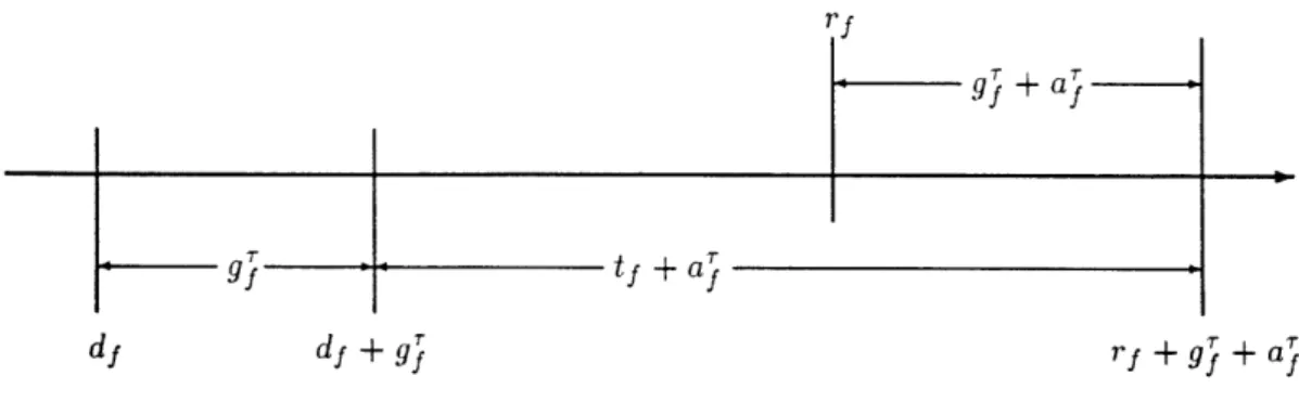
Figure 1: Ground and airborne delays as decided at T.

forecasts extend over the remainder of the time horizon, until time period T, rather than just until the next decision time period '. It will be assumed that these capacity forecasts are perfectly accurate between decision time periods. In other words, the actual airport capacities Dk(t), Rk(t) will be equal to Dk(t), R(t) for t E {r, . . ., }, r E '.

We introduce now the following decision variables: g, f E FT, is the number of time periods for which one decides at r to hold flight f on the ground, before allowing f to take off; a, f E X, is the number of time periods for which one decides at r to delay flight f in the air (e.g., by means of an en route speed reduction), before allowing f to land. At the next decision time period , one may change those decisions that will not have been implemented yet. Nevertheless, at r the situation concerning a flight f E is as depicted in Figure 1.

The actual ground delay of flight f E F will be denoted by Gf. This is a number rather than a decision variable. Its value becomes determined when flight f departs and remains fixed afterwards. Similar remarks hold for Af, the actual airborne delay of flight f.

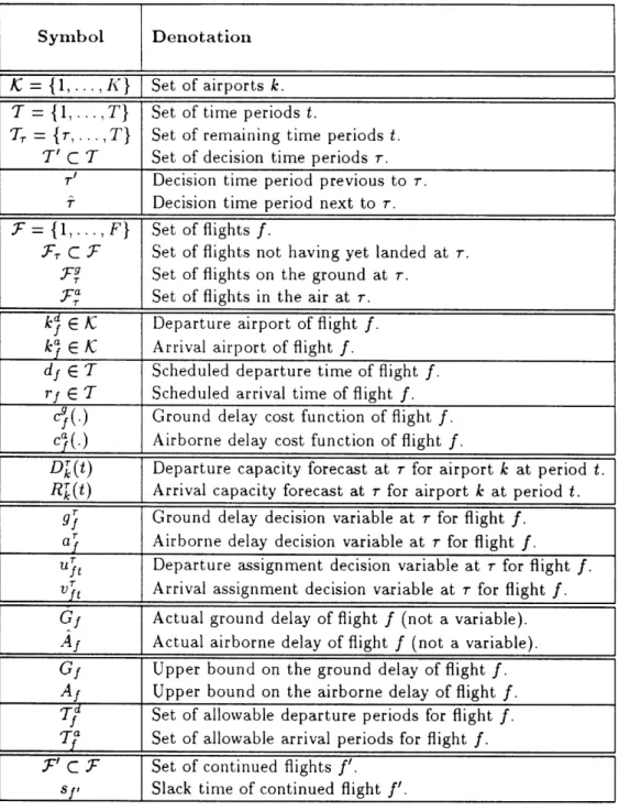
Table 1 summarizes the above notation for reference purposes. Table 1 also includes some symbols which will be defined later on.

Symbol Denotation IK = {1,...,K}

I

Set of airports k. T= {1, .. ,T} Set of time periods t.

T, = Tr,...,T} Set of remaining time periods t.

T' C T Set of decision time periods r.

T' Decision time period previous to r. A Decision time period next to r. F= {1,...,F} Set of flights f.

XC- C F Set of flights not having yet landed at T.

YC~ Set of flights on the ground at T.

OF_ Set of flights in the air at T.

kd E K Departure airport of flight f. k E K Arrival airport of flight f.

df E T Scheduled departure time of flight f.

rf E T Scheduled arrival time of flight f.

(

<.) Ground delay cost function of flight f.

Cf(. ) Airborne delay cost function of flight

f.

D' (t) Departure capacity forecast at for airport k at period t.

R_(t) Arrival capacity forecast at r for airport k at period t. gF Ground delay decision variable at r for flight

f.

ar Airborne delay decision variable at for flight

f.

ut Departure assignment decision variable at for flight

f.

Vt Arrival assignment decision variable at for flight f.

Actual ground delay offlight

f

(not a variable).

Af Actual ground delay of flight f (not a variable).

Af

Actual airborne delay of flight f (not a variable).

Gf Upper bound on the ground delay of flight f.

Af Upper bound on the airborne delay of flight f.

dfSet of allowable departure periods for flight f. f Set of allowable arrival periods for flight f. Fr, C ' Set of continued flights f'.

sf' Slack time of continued flight f'.

rfp + Sf,

slack: s, turnaround time

r'i + Gfo +

Aft

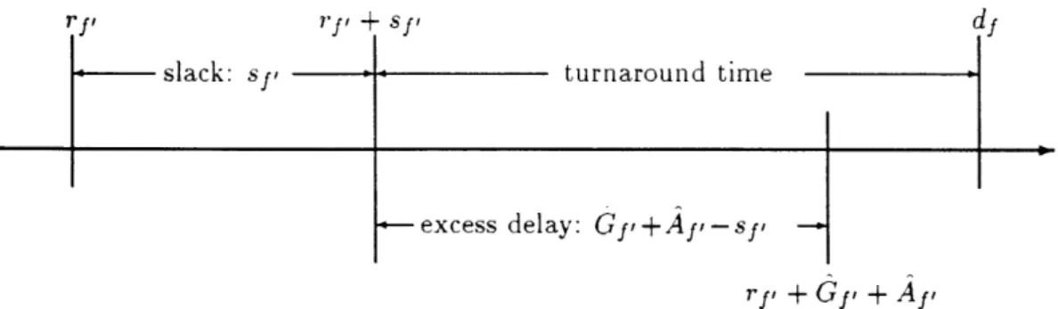
Figure 2: Modeling of coupling constraints.

1.2 Coupling constraints.

Consider the set F' C

F

of those flights that are "continued". A flight is said to be continued if the aircraft which is scheduled to perform it is also scheduled to perform at least one more flight later on in the day. For each flight f' E

F',

we are given the next flight f scheduled to be performed by the same aircraft.

Network effects will be taken into account in the following way. For each continued flight f' E ', we are given the "slack" or "absorption" time sf,. The slack is defined as the number of time periods such that, if f' arrives at its destination at most sfl time periods late, the departure of the next flight f is not affected, whereas if f' lands with a delay greater than the slack, the "excess delay" of f' (i.e., the delay minus the slack) is transferred to the next flight f. In the latter case, the next flight f will incur a ground delay at least equal to the excess delay of

f'.

The situation is depicted in Figure 2, where it can be seen that the slack sf, is equal to the difference between (i) the time interval between the scheduled departure time of f and the scheduled arrival time of f', and (ii) the minimum "turnaround" time of the aircraft performing both flights.

1.3 Assignment decision variables.

The delay decision variables g and a were introduced above. Now we introduce the following assignment decision variables: ut, f E T9, is 1 if one decides at r that flight f will take off at period t (i.e., if rf + g = t) and 0 otherwise; vt, f E .Fr, is 1 if one decides at r that flight f will land at period t (i.e., if rf + g' + a' = t) and 0 otherwise. These new decision variables are introduced because the capacity constraints cannot be expressed in a simple linear way in terms of the more natural delay decision variables.

Moreover, since we do not want to have excessive ground or airborne delays, we also introduce upper bounds on those delays. Gf is the maximum number of time periods that flight f may be held on the ground, and Af is the maximum number of time periods that flight f may be held in the air. Introduction of these bounds results in no loss of generality, since they can be arbitrarily large. In practice, however, typical values are Gf = 4-5 and

Af = 2-3, corresponding to maximum ground and airborne delays of about one hour and

half an hour, respectively.

Given the above setup, the set T7d of time periods to which flight f may be assigned to take off is given by:

T/= {t E T : df < t < min(df + Gf,T). (1)

Similarly, the set Ta of time periods to which flight f may be assigned to land is given by:

fa = {t E T : rf < t < min(rf + Gf + Af ,T)}. (2)

We are now ready to give a first pure 0-1 integer programming formulation of the static deterministic multi-airport GHP.

1.4

A first pure 0-1 IP formulation.

The dynamic formulation consists in solving, at each decision time period r, the following pure 0-1 integer programn:

(IK) min Zfecf cfga + cfaT'EJn

s.t. E kdk < D(t), (k, t) E

Kr

x

T,;

(3) -fE,':k-=k Vft < R'(t), (k, t)E IC x

Tr;

(4) EtETnT uft = 1, f E T; (5) EtETfnz vjt = 1,

f E

17;

(6)

gf + af ,- sf, < g, f' E ' n ;

(7)

Gf + af- sf, < g, f' E n ; (8) a. > 0, f E ; (9) ft, vt E {0, 1}. (10)

The formulation presents a dichotomy necessitated by the fact that flights on the ground at r and flights in the air at r must be treated differently. The objective function is a sum of two terms, corresponding to the ground delay costs of flights on the ground and to airborne delay costs of all flights in FT. (The cost functions cg(t), cf(t) were replaced by their linear

counterparts Ct,

cat

(C, being the constant marginal costs).) The departure capacity constraints (3) and the departure assignment constraints (5) refer only to flights on the ground, while the arrival capacity constraints (4) and the arrival assignment constraints (6) refer to all flights in T,. The coupling constraints (7) and (8) (cf. Figure 2) are also divided into two categories because, for the continued flights f' which are already in the air at r, the ground hold Gf, has already been determined: it is a number, not a decision variable (constraints (8)).

For simplicity of exposition, variables f and a were kept in formulation (Ir), but it should be clear that they can be eliminated by mere substitution in the following way:

9f = tETn T, tuft- d, f E ; 11)

af L tE77fnlT ft- rf - gj, E y; (12)

a = tETfnT, tvt- rf -g f E ; (12)

a- tETnT t - rf - Gf, f E F. (13)

Therefore, the only decision variables are ut and t. The number of these variables for a given is at most ZfEf(2 Gf + Af + 2) (there are at most Gf + 1 ut variables and Gf + Af + 1 vt variables for a given f). For the typical values Gf = 4 and Af = 2, the

number of variables becomes at most 12F, which is a small linear multiple of the number of flights. It can be ssen that the number of constraints is at most 3F+F'+2KT. Thus formulation (I1) is quite compact. Note also that the size of te integer program decreases as increases.

Having solved the program (If7), one solves the program (I^) corresponding to the next decision period by taking as inputs Dk(t), R(t), TI7, and by updating the flight sets as follows:

. = T\ f E T : d + j < T}; (14)

F=)'( Ea\{f : rf +Gf

+a

< })U{f Ef T :(d

+fj < )f)}

(15)

where f and &a are the optimal values returned by (IK1). In words, (14) simply says that the new set of flights on the ground is equal to the previous set of flights on the ground minus the flights that were assigned by (IK1) to leave before the new decision period T.

Similarly, (15) says that the new set of flights in the air is equal to the old set of flights in the air minus any flights in that set that were assigned to land before the new decision period, plus any flights that were previously on the ground, were assigned to depart before

the new decision period, and were assigned to land at or after it.

The final cost resulting from the above dynamic formulation is

ZfEF(cfGf

+caAf). At

T one updates the cost by adding to it the sum of c9 ' for f E {f E F : df + g < }

(i.e., flights which were on the ground at r but left before ), and the sum of ca~ for f E {fE.T :rf+Gf+f < r}U{f E :rf+g+a.f <t} (i.e., flights that either were in the air or were on the ground at r and landed before ). One also sets Gf = gj and Af = a' for flights in the above sets.

An interesting feature of formulation (I ) is that decisions can be updated or overruled as long as they have not been implemented. For instance, aircraft can be assigned ground or airborne delays smaller or larger than what they had been previously assigned, and aircraft not having yet taken off can be given priority over aircraft already in the air. The last possibility is not expected to appear often in the optimal solution, given that c is higher

than Cf. Nevertheless, in practice one would almost never want to deal with this possibility, so formulation (Ir) may be too general. The second dynamic formulation, presented below, always gives aircraft in the air priority over aircraft not having yet taken off.

1.5 A second pure 0-1 IP formulation.

The second formulation assumes infinite departure capacities. For the static case, it has been shown [6,7] that this assumption results in no significant loss of generality if the real deparure capacities are somewhat higher than arrival capacities, as is the case in practice. It has also been shown that, when departure capacities are infinite, if formulation (11) has an optimal solution, then it has an optimal solution in which no flight incurs an airborne delay. In the dynamic case, however, airborne delays cannot be completely eliminated even if departure capacities are infinite. This is because, at a given decision time, the new arrival

capacity forecasts may be significantly reduced with respect to the forecasts of the previous decision time. Then it can happen that even the number of aircraft already in the air exceeds the new capacity forecasts, so that some of these aircraft may have to wait in the air when they arrive at their destination.

For a given decision time period r, define the excess at airport k and time period t, denoted by Ekt, as the number of aircraft currently in the air which will arrive at k at t minus the currently forecasted capacity of k at t. At each decision time period r, one needs to do the following preliminary calculations in order to find what the excesses E are:

BEGIN FOR k = 1 TO K DO: EkT-1- Ek,r-1' FOR t = 7 TO T DO: Ek = max(Ek,t_-,0)+l{ f E) .(ka =k(rf + t)l R-(t)

CONTINUE t

CONTINUE END

Ekr-1 are the excesses calculated at r', the decision time previous to . (At decision

time 1, one 1, one begins with Eo = 0.) These previously calculated excesses are the actually

realized excesses, since capacity forecasts at r' are accurate until r - 1. Any positive excess at a time period t - 1 is transferred to the next time period t. As a result of the above preliminary calculations, if E't < 0, then -Ekt is the available arrival capacity of airport k at time period t, i.e., the currently forecasted capacity minus the number of aircraft that

are already in the air and will arrive at k at t. On the other hand, if Et > 0, then there is no available capacity at k at t, and the best one can do, supposing that aircraft in the air have priority over aircraft on the ground, is to not assign any of the aircraft currently on the ground to arrive at k at t.

Another preliminary calculation which needs to be carried out at each decision time period concerns the unavoidable airborne delays of flights already in the air, arising when the new capacity forecasts are not sufficient to accommodate these flights. These delays, which will be denoted by aj (numbers, not variables), will be needed for the coupling constraints and for the calculation of the total cost. They are calculated by means of the excesses E't in the following way:

BEGIN FOR f C T DO:

~f

T 1 CONTINUE f FOR k = 1 TO K DO: FOR t = TO T DO: IF E't > 0 THEN

Select Ekt flights in {f E (kf = k)(rf+gf +cf =t)} and

set c = a + 1 for them. END IF

CONTINUE t

CONTINUE k END

The selection of the flights to be delayed depends on the arrival queueing discipline, usually FCFS.

We are now in the position to give the second dynamic deterministic formulation, with infinite departure capacities:

(I2) min f E' Cfgf s.t. Efef?:k~= k vjt < max(-Et ,0), (k,t) IC x T; (16) EteTnT vTt = 1, f C .Fg; (17) gj,- sf, < g, f' n ,; (18) Go + 7a,-

g,

gI f

n

a; (19) v t {0 , (20) where: 9g

=

S

tvjt -

rf,f cg. (21) tETSn,r

Constraints (16) say that, if Er < 0, then the number of aircraft assigned to arrive at airport k at time period t must not exceed the available excess capacity -Ert; whereas, if Ek > 0 (i.e., no available capacity at k at t), then vft will be 0 for all f that could arrive at k at t, so that no new aircraft will be assigned to arrive at k at t. Note that decisions are taken only for flights on the ground at r. Flights in the air at r influence the decisions by means of (16) (by determining the excesses) and of (19) (their airborne delays enter into the coupling constraints).

The total cost is calculated and updated at each decision time period in a way analogous to that explained in the previous subsection for formulation (Ir).

2

Extensions of the deterministic formulations.

2.1

Flight cancellations.

In situations where delays become excessive, it is common airline practice to cancel some flights, especially at hub airports. Motivated from this fact, we developed formulations which take into account the possibility of cancelling flights. These formulations have the additional advantage that they escape infeasibility problems which might arise with formu-lations (IT) and (12). Infeasibility occurs when airport capacities are low: even though the total daily capacity of an airport may be sufficient to accommodate the total number of flights scheduled to depart from or arrive at that airport, the problem may still be infeasible if excessive congestion appears during some portion of the day.

We will give will give a formulation (I3) generalizing (I). Keep the old decision variables utt and ft and define the new decision variables zf f C ., to be 1 if flight f is cancelled at r and 0 otherwise. Denote by Mf the cancellation cost of flight f. When a flight in F'

(i.e., a flight that is "continued") is cancelled, there are two possibilities concerning the next flight initially scheduled to be performed by the same aircraft: either it is performed by a replacement (or a "spare") aircraft, or it is also cancelled. The first case is more common in practice, especially in hub airports where most cancellations take place, but the formulation is general enough to incorporate a combination of both cases. Partition T' into

FT,

the set of those flights in F' whose cancellation will not affect their next flight, and ~}, the set of those flights in F' whose cancellation will entail the cancellation of their next flight. At r solve:

(I3) min _{fEg (cgf + (Mf + cg rf)j)}

Zfj + EtEnrfan Vt = 1,

f

C fT;

(22)

g,- Sf1 + (s, + 'f, - rf)zf, • g< , f

C

.T'₁n T;

g,-sf +(sf

+

rf

+

Gf + 1)Zf, g + (rf + Gf + 1) f' E 2

n

;

2Vjt,Zj E {0, 1}.

where g are given by (21).

The above formulation incorporates some technical tricks which are necessitated by the fact that, when a flight f is cancelled (i.e., z = 1), then all v _t corresponding to f are 0

(by (22)), so that (21) gives g = -f. Keeping this fact in mind, it can be seen immediately that, when z = 1, the objective function term corresponding to f is Mf. One can similarly simplify the coupling constraints when zj, = 1.

The variables gj were again left in the formulation, but it should be clear that they can be eliminated by mere substitution through (21). Now an important point is that the variables zj can also be eliminated through (22), provided that (22) is replaced by

EtlEnfl V < 1.

The fact that the new formulation (I3) has exactly the same number of variables and of constraints as (2) is particularly significant, since (13) enjoys considerable advantages both in terms of generality (the real-world problem is better approximated) and in terms of flexibility (infeasibility problems are eliminated).

2.2 Interdependent departure and arrival capacities.

The departure and arrival capacities of a given airport at a given time period are often not independent, because they are determined by the way in which runway use is allocated among departing or arriving aircraft. If all runways are exclusively used for landings,

rkt

Rk,max (t)

3Dk,max(t)

dkt

Dk,max(t)

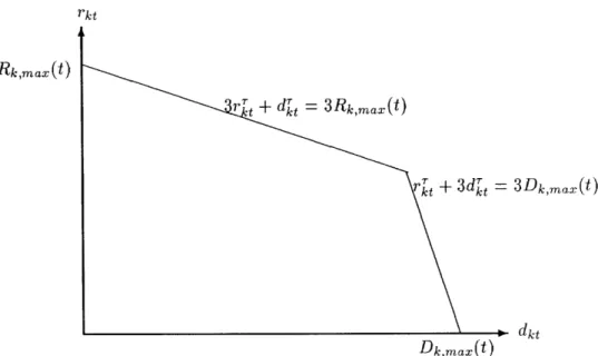
Figure 3: An example of a region of possible combinations between the departure capacity dt and the arrival capacity rt of airport k at time period t, as forecasted at r.

arrival capacity reaches a maximum value Rk,max(t) determined by the minimum separation between successive landings, while departure capacity is 0. If all runways are exclusively used for take-offs, departure capacity reaches a maximum value Dk,max(t) determined by the minimum separation between successive take-offs (which is less than the minimum separation between landings, so that Dk,max(t) > Rk,max(t)), while arrival capacity is 0. Intermediate cases give departure and arrival capacities belonging to a region with the general shape of a two-dimensional convex polytope (Figure 3). Note that this region differs among airports and, for a given airport, it can change with time (because weather can change).

The above situation can be easily taken into account by generalizing formulation (I,). This is achieved by introducing the new integer (not 0-1) decision variables dkt and rkt standing, respectively, for the departure and the arrival capacities of airport k at time t, as forecasted at r. These new decision variables will replace the constants D'(t) and RL(t)

in the right-hand sides of the capacity constraints. In addition, new sets of constraints will be needed, one set for each time period, ensuring that dt and r fall within the region of their possible combinations. These constraints will be of the following general form:

ozktdkt +13 ktrkt _{kt ktt} < -''t ykt (k,t) x i 1,.. .,Ikt (23)

where atkt3", kt, kt are constants and Ikt is the number of linear constraints describing the departure-arrival capacity region of airport k at time period t, as forecasted at r. For instance, for the region shown in Figure 3, the following two constraints are needed for period t:

3_{rt + dkt < 3Rk,max(t); (24)}

rt + 3dt < 3Dk,max(t) (25)

Variables dt and rt can be eliminated. In fact, the departure and arrival capacity constraints (3) and (4) can be replaced by equalities since constraints (23) are inequalities. Then dkt and r t will represent the used capacities of airport k at time period t, as forecasted at r. Thus constraints (3) and (4) will be removed from (I ) and will be replaced by:

ciT( TJ + vkt(

S

vt) < 7 (k,

t)

x , i{1,...,

I

f:kd=k f:k =k

It is remarkable that this generalization of (I ) has exactly the same (number of) variables as (I,) and only slightly more constraints.

2.3 Further extensions.

2.3.1 Hub airports: more than one "next" flights.

In hub airports, an arriving flight typically has passengers connecting to several departing flights. This can be taken into account in any of the above formulations by means of an

easy extension. It suffices to reinterpret the coupling constraints as linking not only a pair of flights scheduled to be performed by the same aircraft, but also any pair of flights f' and

f

such that f is not allowed to leave before

f'

lands, because passengers in

f'

connect to

f. With this reinterpretation of the coupling constraints, a continued flight may have more

than one next flights. Therefore, the formulations remain unchanged and a number of new coupling constraints is simply added to them.

Note that the slack in a coupling constraint of the new kind (connecting flights) will typically be different from the slack in a coupling constraint of the old kind (continued flights). This is because the turnaround time involved in connecting flights is restricted to moving passengers and their luggage, while the turnaround time involved in continued flights also includes cleaning and refuelling the aircraft.

2.3.2 En route speeding.

Sometimes there is the possibility to speed up an aircraft en route, so that the aircraft may arrive even before its scheduled arrival time. This possibility can be easily taken into account in any of the formulations with airborne delays presented in this chapter. It suffices to take rf to be not the scheduled arrival time, but the earliest possible arrival time. If, for instance, an aircraft is scheduled to arrive at time period 28, but may be speeded up so as to arrive up to two periods earlier, rf for the corresponding f will be equal to 26. An airborne "delay" A1 equal, e.g., to 1 will correspond to a speeding up of one time period,

whereas an Af equal to 3 will correspond to a slowing down of one time period. The actual arrival time of flight f will of course also depend on its ground delay: if f departs with a ground delay Gf equal to 3 and is speeded up by one time period, it will arrive with a total delay of two time periods, i.e., at period 30 (which is rf + Gf + A = 26 + 3 + 1). Note that

the upper bound Af will have to be increased by 2 in this example.

3

Probabilistic formulations.

One way to model the case of probabilistic capacities is by considering that capacity fore-casts take the forms of various scenaria, each scenario coming with a given probability of realization. In symbols, there are L possible capacity scenaria, and scenario 1, having probability pI (=I PI = 1), is denoted by RI(t), (k,t) E K x T. Note that a capacity scenario involves capacity forecasts for all airports of the network. In other words, pi is the probability that airport 1 will have capacities RI (t), t G T, and that airport 2 will have capacities RI (t), t E T, and so on. This is because capacities at various airports may not be independent, especially for airports close enough to have similar weather.

In the probabilistic GHP, static policies are subject to a "paradox" which does not appear in the deterministic GHP. At the beginning of the day, one knows the possible capacity scenaria and their probabilities of realization, but of course one does not know which scenario will be realized. If the problem is static, one must make irrevocable decisions concerning ground holds at the beginning of the day. But sooner or later some scenario will be realized, and at that point one should normally take into account the new information and update ground holds. So the paradox of the static probabilistic GHP is that new information will inevitably become available but will not be taken into account. The static deterministic GHP encounters no similar problem because, by assumption, capacity forecasts are perfectly accurate and no new information will become available.

The above considerations show that static probabilistic formulations may be of some-what limited practical interest in themselves. Nevertheless, they can be used as building blocks for dynamic probabilistic formulations. This is entirely analogous to the way in

which the static deterministic formulations of [6] were used as building blocks for the dy-namic deterministic formulations of Section 1. As an example, we will present below, for the case of infinite departure capacities, a static probabilistic formulation and its dynamic extension.

3.1

A static probabilistic formulation.

Define the decision variables gf, equal to the ground delay of flight f, and vft, equal to 1 if scenario I is realized and flight f lands at t, and equal to 0 otherwise. Denote also by al the airborne delay of flight f if scenario I is realized. Under scenario 1, the total delay of flight f, gf + a, is equal to the difference between the actual arrival time, t tvt, and

fight~

f,

g + Zr~a ft,

the scheduled arrival time, rf, so that:

a

tvft

- rf -gf, f T, E {1,...

L}.

(26)

teTvf

Assuming infinite departure capacities, we have now the following static probabilistic IP formulation:

(Ip) min yfe(cfgf + Cca

I=

plal )

s.t. Ef:k=k Vft <

R

(t), (k,t) C x T, 1 .1,..

,

L}; (27)

Et~VIOft = lo

f

C

A,

e

{1,

,L};

(28)

gf + a ,s- Sf < gf ' ', {1,.,L}; (29)

gf {0,1,...,Gf}, f E ; (30)

vtft C {0, 1}. (31)

Although formulation (Ip) looks superficially similar to previously presented formulations, it has several peculiarities which need mentioning. By solving (Ip), one gets values for gf and vft. The values for gf are the ground holds which will be implemented no matter which

capacity scenario is ultimately realized, since we are examining the static case. On the contrary, which values vft will be implemented will depend on the capacity scenario that will be realized. If, for instance, scenario 3 is realized, then flight f will land at the time

period t for which vft is equal to 1. Therefore, it can be seen that gf cannot be expressed

in terms of vt: there are two independent sets of decision variables. Moreover, (Ip) is not a pure 0-1 IP formulation, since gf are not binary variables.

Another important comment concerns the coupling constraints (29). These must ensure that the ground holds gf, which are irrevocably decided at the beginning of the day, will be feasible no matter which capacity scenario is ultimately realized. But the capacity scenario which will be realized may affect the airborne delays of continued flights, which may in turn affect the ground delays of their next flights. This problem is solved, in (29), by having the ground delay of a continuing flight be at least equal to the maximum excess delay of its previous flight over all possible capacity scenaria.2

A final remark concerns the size of formulation (Ip). There are LKT + (L + 1)F + LF' constraints, and the number of decision variables is at most F + =L1 Ef ejr(Af + 1), where Af is an upper bound on the airborne delay of flight f under scenario 1. Such an upper

bound cannot be arbitrarily imposed, but can be calculated for given arrival profiles and capacity scenaria. In the worst case, A = T- rf will do. Therefore, the number of

constraints and the number of variables can become excessive, expecially if L is large, but may remain manageable for small L.

Extensions of formulation (Ip) like those presented in Section 1 (e.g., with flight can-cellations) are straightforward.

3.2

A dynamic probabilistic formulation.

Extending the static probabilistic formulation of the previous subsection to the dynamic probabilistic case is rather straightforward, but there is a minor complication. The compli-cation concerns the way of modeling the additional information that emerges as time goes on. In an extreme case, one of the possible capacity scenaria is realized at a time and all uncertainty is eliminated after that time. In a more realistic case, at various realization

time periods 6 E A C T the probabilities of the various scenaria are updated to p. In this case the reasonable thing to do is to identify the set of decision time periods T' with the set of realization time periods A, since it is exactly at realization time periods that new information becomes available.

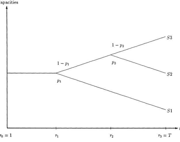
The situation can be explained with the help of Figure 4, which refers to a case with L = 3 capacity scenaria and is also the basis of the computational results presented in Chapter 5.3 At time r0 = 1, one knows that scenaria S1, S2, S3 will be ultimately realized

with probabilities p = P1, P2 (1 - )P, p = (1 -p l)(l -P2), respectively. (Moreover, one knows the capacities with certainty until time r, since all three scenaria coincide until that time.) So at r0 one solves formulation (Ip) with pO as above. Now at time 71 new information is obtained: either scenario S1 is realized or it is not. This new information gives pl. If S1 is realized, then p' = 1 and p 1 = O. If S is not realized, then Pl = 0, P1 = P2, and p = 1- P2. So at r1 one solves formulation (Ip) with p as above.4 Similarly at r2.

We give now the dynamic probabilistic formulation corresponding to (Ip). The notation

3

As was pointed out above, a capacity scenario includes capacity forecasts for all airports of the network. Figure 4 gives only the parts of scenaria S1, S2, and S3 that correspond to a given airport.

4

Capacities

S3 1 - p2 1 - Pl S2 P1 S1 t ro = 1 T1 r2 r3 = T

Figure 4: Modeling additional information over time in the dynamic probabilistic GHP. There are three possible capacity scenaria: S1, S2, and S3. Overall, SI has lower capacities than S2, and 52 has lower capacities than S3. All three scenaria coincide between time periods

r

0 and 71, and scenaria S2 and S3 coincide between time periods 71 + 1 and r2.

At rl, S1 is realized with probability pl and all uncertainty is eliminated. Otherwise (with probability 1-pi), at r2, S2 is realized with probability P2 or S3 is realized with probability 1 - P2.

generalizes that of Section 1 (cf. Table 1).

(Ip)

min

fE-g c9f +

f E, cf 1=

₁

Pa

f

s~t. _{Ef ErT:k-=k Vft -k} 1 lv<

R 1

7(t

_(),

(k₍

f

ZtET7nT,- V~= 1,7 g;, + a, - sI < g, '

(O,

+ a /, < g, '

g E{O,1,

...,Gf},

f

V1t

E {O, 1, where: fac = E tVf -rf-gf, fE , X tEfanr a =v tV - rf -Gf, f E

T,

l tETfafnr

This concludes the presentation of the formulations. computational results based on the above framework.

,t)ECxT, e{l,, L};

E

X

E

g,

1,...,

L};

E

;'n.T',

e {1, . ,

L ;

'E .; (32) (33) (34) (35) (36) (37) (38) (39) (40)

The next section will present

4

Structural insights.

4.1

Comparing dynamic scenaria.

The goal of this section is to gain insight on the behaviour of the dynamic multi-airport

GHP by examining a relatively realistic case with three capacity scenaria and two realization

times (identical with the two decision times), on the model of Figure 4. The computations

will be carried out with formulation (2). In the most general case (see Figure 4), one solves

first (I2

°

) with capacity forecasts equal to S1 or S2 or S3, for t E {1, . . ,T}. Then one

E II,_, LI;

solves (I2') with new capacity forecasts (e.g., S2 or S3 if the previous forecast was SI), but now for t E {r7,...,T}. Finally one solves (2) with yet new capacity forecasts and for t E {r2,.. ., T}. In special cases, one may not need to solve (Il ), (I2 ), or both, if

the capacity forecast does not change. Suppose, for instance, that the forecast at 70 is S2 and that S1 is realized at r1. Then one needs to solve (I2') with forecast Si, but no new

problem needs to be solved at T2, since the forecast will inevitably remain S1.

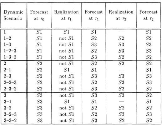
A particular combination of (at most three) problems to be solved in the dynamic case will be referred to as a (dynamic) scenario (not to be confused with a capacity scenario, which is one of S1, S2, S3). In the example at the end of the last paragraph, the dynamic scenario will be referred to as 2-1, since one solves (2 °_{) with forecasts S2 and then (I2')} with forecasts S1. Some reflection should convince the reader that, assuming all branches in Figure 4 have nonzero probabilities, there are 15 possible dynamic scenaria that one may have to solve, depending on which capacity scenaria are forecasted and which are realized. These 15 dynamic scenaria are given in Table 2.

To be quite explicit, the relationship between the "forecast" and the "realization" columns of Table 2 is the following: only a capacity scenario which can be realized may be forecasted, and any capacity scenario which can be realized may be forecasted. At To, for

instance, all three capacity scenaria are possible, so any of them may be forecasted. At 1, if S1 is realized, then only S1 can be forecasted, whereas, if SI is not realized, then either S2 or S3 may be forecasted. In practice, of course, which capacity scenario will be fore-casted will depend on the probabilities of the branches in Figure 4 and on the forecasting method (e.g., most-probable, worst-case, etc). Probabilities and forecasting methods will be introduced in the next section; for the moment we are just examining all possible cases. We want to examine the possible dynamic scenaria before introducing probabilities of

Table 2: The 15 possible dynamic scenaria (cf. Figure 4-1).

realization because there are interesting and insightful comparisons to be made. As an example, the cost of scenario 3 must be lower than (or equal to) the cost of scenario 3-3-2, because in 3-3-2 the new capacity forecasts at r2 are lower than the previous forecasts, so some already departed aircraft may have to wait in the air. In other cases the comparison is less clear. Compare, for instance, the costs of scenaria 1-2-3 and 1-3-2. At r2 some departed aircraft in 1-3-2 may have to wait in the air, while this is not the case in 1-2-3. But the departed aircraft in 1-3-2 have probably had lower ground holds than in 1-2-3, since the previous capacity forecasts were more optimistic in 1-3-2 than in 1-2-3. There is thus a trade-off between ground and airborne delay costs, and it is interesting to pursue the investigation further.

Computational experiments were performed for four cases with K = 3 airports and F = 1500 flights. All cases have the same profile of scheduled arrivals but different percentages

Dynamic Forecast Realization Forecast Realization Forecast

Scenario at ro0 at rl at r1 at 2 at 2 1 S1 Si S1 S1 1-2 S1 not S S2 S2 S2 1-3 S1 not S1 S3 S3 S3 1-2-3 Si not S1 S2 S3 S3 1-3-2 S1 not S1 S3 S2 S2 2 S2 not S1 S2 S2 S2 2-1 S2 S1 S1 - S1 2-3 S2 not S1 S3 S3 S3 2-2-3 S2 not S1 S2 S3 S3 2-3-2 S2 not S1 S3 S2 S2 3 S3 not S1 S3 S3 S2 3-1 S3 S1 S1 S1 3-2 S3 not S1 S2 S2 S2 3-2-3 S3 not S1 S2 S3 S3 3-3-2 S3 not S1 S3 S2 S2

of continued flights, F'/F, ranging from 0.20 to 0.80. The four cases are comparable, in the sense that cases with lower F'/F are obtained from cases with higher F'/F by eliminating some connections between flights. All four cases have slacks equal to 0 and identical arrival capacity profiles in the spirit of Figure 4, with the difference that S2 has a positive slope and S1 is constant (rather than S1 and S2 having negative slopes, as they have in Figure 4). S1 is at the infeasibility limit, and is equal to 11, 10, and 10 aircraft per time period for airports 1, 2, and 3, respectively. The two realization and decision times are 1 = 21 and r2 = 41; the time horizon has T = 64 time periods. Ground delay costs are 50 and airborne delay costs are 75.

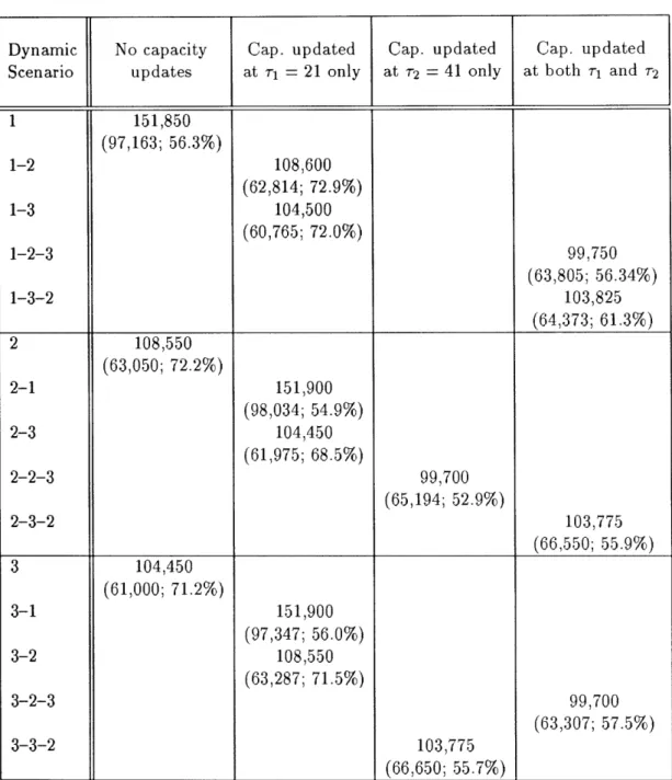
The results of the computations are shown in Tables 3 and 4. It should be noted that the computations were performed with the LP relaxation (L7) rather than (If), because the values of (L2) and (I') are very close for identical cost functions [6,7]. Nevertheless, rounding mistakes are expected.

After some reflection, one can make the following observations on the basis of Tables 3 and 4. First, the 15 dynamic scenaria fall into two groups, call them group A and group B. Group A has three subgroups of three scenaria each. Subgroup Al consists of scenaria 1, 2-1, and 3-1; subgroup A2 consists of scenaria 2, 1-2, and 3-2; and subgroup A3 consists of scenaria 3, 1-3, and 2-3. It can be seen that, for any of the four values of F'/F, all three scenaria within any of the above three subgroups have equal values. In symbols, we always

have:

V1 = V2-1 = V3-1 > V2 = V1-2 = 3-2 > V3 = V11-3 = V2-3- (41)

Why should this be so? The reason is probably that all scenaria within the above subgroups (with the exception of the static scenaria 1, 2, 3) have capacity updates only once, and at a rather early time period (r1 = 21 with T = 64). Recall that all three

Dynamic No capacity Cap. updated Cap. updated Cap. updated Scenario updates at r1 = 21 only at r2 = 41 only at both rl and r2

1 50,550 1-2 35,700 1-3 32,250 1-2-3 32,500 1-3-2 35,850 2 35,700 2-1 50,550 2-3 32,250 2-2-3 32,500 2-3-2 35,850 3 32,250 3-1 50,550 3-2 35,700 3-2-3 32,500 3-3-2 35,850 1 50,550 1-2 36,100 1-3 32,800 1-2-3 32,400 1-3-2 35,200 2 36,100 2-1 50,550 2-3 32,800 2-2-3 32,667 2-3-2 35,775 3 32,800 3-1 50,550 3-2 36,100 3-2-3 32,869 3-3-2 34,950 Table 3: Values for F'/F = 0.40

of the 15 dynamic scenaria for F'/F = 0.20 (upper part of the table) and (lower part).

Dynamic No capacity Cap. updated Cap. updated Cap. updated Scenario updates at r1 = 21 only at r2 = 41 only at both r1 and r2

1 63,188 1-2 40,250 1-3 35,750 1-2-3 37,895 1-3-2 38,574 2 40,250 2-1 63,188 2-3 35,750 2-2-3 36,020 2-3-2 40,092 3 35,750 3-1 63,188 3-2 40,250 3-2-3 37,013 3-3-2 38,447 1 70,500 1-2 46,100 1-3 40,150 1-2-3 42,974 1-3-2 45,922 2 46,100 2-1 70,500 2-3 40,150 2-2-3 41,315 2-3-2 44,755 3 40,150 3-1 70,500 3-2 46,100 3-2-3 41,337 3-3-2 46,700 Table 4: Values for F'/F = 0.80

of the 15 dynamic scenaria for F'/F = 0.60 (lower part).

capacity scenaria coincide until rl. In conclusion, (41) seems to say that, if one can get the

correct capacity forecasts early enough in the day, one can almost completely compensate for incorrect capacity forecasts made at the beginning of the day. It should be noted that

one does not always expect the equalities (41) to hold exactly. For instance, scenario 3-2 can sometimes have a higher value than scenario 2, because some aircraft in the air at r1 may have to incur airborne delays when the forecast shifts from S3 to S2.5

The second group, group B, consists of two subgroups of three scenaria each. Subgroup B2 consists of scenaria 1-3-2, 2-3-2, and 3-3-2; subgroup B3 consists of scenaria 1-2-3, 2-2-3, and 3-2-3.6 These subgroups are detected by means of the case F'/F = 0.20 (upper part of Table 3), where all scenaria within each of these two subgroups have equal values.

In symbols:

Vl_2_₃ V2-2--= ₃ 3_2_3 < v1_3_₂ = v22_3_2 = v3_3_2, for F'/F = 0.20. (42)

Examination of the other three cases for F'/F supports (42), although the equalities become approximate.

The equalities in group B have presumably the same origin as those in group A: incorrect forecasts are corrected early enough, so that their influence is minimized. Scenaria within each subgroup of group B (e.g., scenaria 1-2-3 and 3-2-3) differ only up to time r1 = 21.

One can also compare scenario 3 with 2-2-3, or scenario 2 with 3-3-2. Here we have incorrect predictions which are corrected late in the day (at r2 = 41 with T = 64). It is seen

that only minor differences appear. In other words, the values of scenaria within subgroup B2 are quite close to the values of scenaria within subgroup A2 (similarly for subgroups B3

5

For an example of a case where (41) do not hold exactly, see Table 7.

6

The reason why the two subgroups of group B were named B2 and B3, rather than B1 and B2, is that subgroups B2 and A2 (and, similarly, subgroups B3 and A3) share an important feature: all scenaria within B2 and A2 end in 2. In other words, all six scenaria in these two subgroups correspond to the case where capacity scenario S2 is ultimately realized.

and A3). Therefore, it seems that obtaining the correct capacity forecasts even relatively late in the day suffices to minimize the impact of incorrect capacity forecasts made at the beginning of the day.

The main result of this subsection is that, if one obtains the correct capacity forecasts before the end of the day, then one can, for the most part, compensate for incorrect capacity forecasts made earlier on. Referring again to Figure 4, one can understand the reason. The difference between different dynamic scenaria is mainly due to aircraft which may have to wait in the air when the new forecast is lower than the previous one. Such aircraft are in the air at the current decision time period, so they will arrive at their destination soon. So the only differences between capacity scenaria that really matter are the differences in the vicinity of decision time periods. But such differences are usually small, because the capacity scenaria usually diverge smoothly rather than abruptly. This is why dynamic scenaria ending in i will have values quite close to vi. What mostly matters is to obtain the correct forecasts, not when to obtain them.

4.2 Comparing forecasting methods.

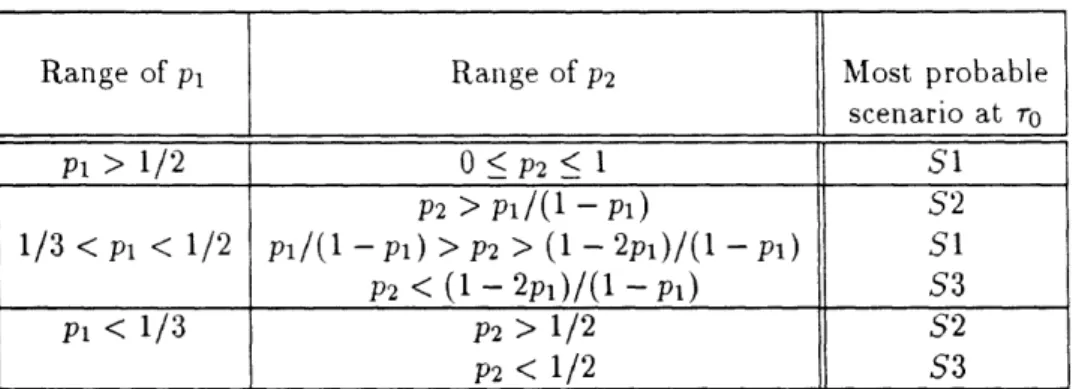
Two forecasting methods will be examined: the most-probable forecast and the worst-case forecast. Referring again to Figure 4, at time T₀ the most-probable forecast is S1 if P > 1/2, while it is S2 if p < 1/3 and P2 > 1/2. All possible cases are given in Table 5. Similarly, at 71, supposing S1 is not realized, S2 is most probable when P2 1/2. The worst-case forecast, on the other hand, is obviously S1 at r₀ and, if S1 is not realized, S2 at rl.

For given values of the probabilities P1 and p2, the expected value of the policy which uses the most-probable forecast is:

Table 5: Most probable capacity scenario at r0 for various probability combinations (cf. Figure 4).

where v(MPli) is the value of the dynamic policy given that capacity scenario i is ultimately realized. For instance, if S2 is realized and P1 > 1/2, P2 < 1/2, the most-probable forecasts will be S1 at r0 and S3 at r, so that vMPi2 = vl-3-2. It is seen that MPli depends not

only on i but also on P1 and P2.

For given values of the probabilities P1 and P2, the expected value of the policy which uses the worst-case forecast is:

WC = pivVwc11 + (1 - pl)p2vwcl2 + (1 - pl)(l - P2)Vwc3 (44)

It is easily seen that, for the case of Figure 4, vwcl = Vl, vwcl2 = v 2, and Vwcl3 = l

1-2- 3, regardless of the values of P1 and P2

In order to compare the dynamic with the static GHP, we also included in the comparison the expected value of a random-selection static policy:

RS = pvi + (1 - pl)p2v2 + (1 - pl)(1 -p2)v3, (45)

where vi is the value of scenario i. The random-selection static forecast is defined by means of a probabilistic event: at To, one performs an experiment which yields outcomes 1, 2, and 3, with probabilities Pl, (1 - p)P2, and (1 -pl)( -P2), respectively. If outcome i E {1, 2, 3} occurs, then the random-selection forecast is Si, and is not updated at later decision times.

Range of pi Range of P2 Most probable

scenario at To P > 1/2 0 < 2 l 1 S1 p2 > p1/(l - Pl) S2 1/3 < P1 < 1/2 pi/(l - pl) > P2 > (1 - 2p1)/(l - pi) S1 _ P2 < (1 - 2p)/(l - pi) S3 P < 1/3 P2 > 1/2 S2 P2 < 1/2 S3

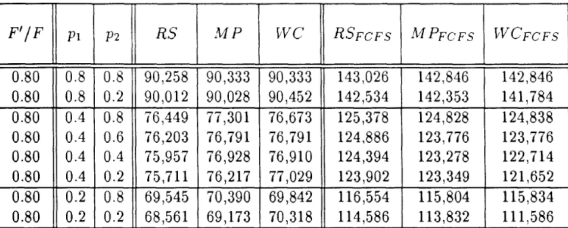
Table 6 gives the expected values of the two dynamic policies under consideration and of the static random-selection policy for typical values of P1 and P2 corresponding to the combinations of Table 5. It is seen that the expected values of both dynamic policies are always very close to the expected value of the random-selection policy and to each other. It seems, therefore, that both forecasting methods perform equally well. On the other hand, the dynamic policies seem to result in no significant cost savings over the static random-selection policy.

These results were expected, given the conclusion of Subsection 4.1. In fact, MPli and

vWCli are always close to vi, so (43), (44), and (45) entail the approximate equality of MP, WC, and RS.

4.3 A dynamic FCFS heuristic.

The following dynamic heuristic is inspired by current ground-holding practice. It gives priority to aircraft in the air over aircraft on the ground, and it assigns available capacity on an FCFS basis.

BEGIN

Initialize: gf = 0.

FOR t = TO T DO:

FOR k = 1 TO K DO:

FOR f E 7EY DO:

IF k = k AND rf + Gf + af = t AND f has a next flight f THEN g = max(Gf + af - s, 0). Similarly if j has a next flight and so on.

F'/F Pl P2 Random-selection Most-probable Worst-case 0.20 0.8 0.8 47,442 47,452 47,452 0.20 0.8 0.2 47,028 47,586 47,068 0.20 0.4 0.8 41,226 41,256 41,256 0.20 0.4 0.6 40,812 40,872 40,872 0.20 0.4 0.4 40,398 40,434 40,488 0.20 0.4 0.2 39,984 40,002 40,104 0.20 0.2 0.8 38,118 38,158 38,158 0.20 0.2 0.2 36,462 36,486 36,622 0.40 0.8 0.8 47,528 47,512 47,512 0.40 0.8 0.2 47,132 47,096 47,068 0.40 0.4 0.8 41,484 41,276 41,436 0.40 0.4 0.6 41,088 40,992 40,992 0.40 0.4 0.4 40,692 40,476 40,548 0.40 0.4 0.2 40,296 40,158 40,104 0.40 0.2 0.8 38,462 38,441 38,398 0.40 0.2 0.2 36,878 36,694 36,622 0.60 0.8 0.8 58,420 58,506 58,506 0.60 0.8 0.2 57,880 57,813 58,224 0.60 0.4 0.8 48,885 48,918 49,143 0.60 0.4 0.6 48,345 48,860 48,860 0.60 0.4 0.4 47,805 47,403 48,577 0.60 0.4 0.2 47,265 47,049 48,295 0.60 0.2 0.8 44,117 44,161 44,461 0.60 0.2 0.2 41,958 41,669 43,330 0.80 0.8 0.8 65,382 65,495 65,495 0.80 0.8 0.2 64,668 64,661 65,160 0.80 0.4 0.8 55,146 55,286 55,485 0.80 0.4 0.6 54,432 55,110 55,110 0.80 0.4 0.4 53,718 53,675 54,735 0.80 0.4 0.2 53,004 53,076 54,360 0.80 0.2 0.8 50,028 50,214 50,480 0.80 0.2 0.2 47,172 47,268 48,979 Table 6: Expected various probability

values of dynamic policies combinations.

Define Sk(t) := {f E f: (k = )(rf + gf =

t)}

Define Sk(t):= ISk(t)l.

IF Sk(t)> -Ek(t) THEN:

Choose Qk(t) := Sk(t) + min(Ek(t), 0) flights in Sk(t). FOR f = 1 TO Qk(t) DO:

Set gf = gf + 1.

IF f has a next flight

f

THEN: IF gf > Sf THEN:

Set g = g + 1, and similarly if

f

has a next flight and so on.

END IF END IF CONTINUE f END IF CONTINUE k CONTINUE t END

Computations were performed for the same case as in Subsection 4.1 (3 airports and 1500 flights), but only for F'/F = 0.80, and with slacks equal to 1 instead of 0. The new capacity scenaria are lower, since the infeasibility limit is lower (due to the increase of the slack). The new S1 is equal to 10, 9, and 9 aircraft per time period for airports 1, 2, and